The
JWST Extragalactic Mock Catalog: Modeling Galaxy Populations from the UV
through the Near-IR over 13 Billion Years of Cosmic History
Christina C. Williams1,15 , Emma Curtis-Lake2, Kevin N. Hainline1 , Jacopo Chevallard2, Brant E. Robertson3 , Stephane Charlot2 , Ryan Endsley1, Daniel P. Stark1, Christopher N. A. Willmer1 , Stacey Alberts1, Ricardo Amorin4,5 , Santiago Arribas6, Stefi Baum7, Andrew Bunker8, Stefano Carniani4,5 , Sara Crandall3, Eiichi Egami1, Daniel J. Eisenstein9, Pierre Ferruit10, Bernd Husemann11 , Michael V. Maseda12 , Roberto Maiolino4,5, Timothy D. Rawle13, Marcia Rieke1,
Renske Smit4,5 , Sandro Tacchella9 , and Chris J. Willott14
1
Steward Observatory, University of Arizona, 933 North Cherry Avenue, Tucson, AZ 85721, USA;[email protected]
2
Sorbonne Universités, UPMC-CNRS, UMR7095, Institut d’Astrophysique de Paris, F-75014, Paris, France;[email protected]
3
Department of Astronomy and Astrophysics, University of California, Santa Cruz, 1156 High Street, Santa Cruz, CA 95064, USA
4
Cavendish Laboratory, University of Cambridge, 19 J.J. Thomson Avenue, Cambridge CB3 0HE, UK
5
Kavli Institute for Cosmology, University of Cambridge, Madingley Road, Cambridge CB3 0HA, UK
6Departamento de Astrofisica, Centro de Astrobiologia, CSIC-INTA, Cra. de Ajalvir, E-28850-Madrid, Spain 7
University of Manitoba, Department of Physics and Astronomy, Winnipeg, MB R3T 2N2, Canada
8
Department of Physics, University of Oxford, Oxford, UK
9
Harvard-Smithsonian Center for Astrophysics, 60 Garden Street, Cambridge, MA 02138, USA
10Scientific Support Office, Directorate of Science, ESA/ESTEC, Keplerlaan 1, 2201AZ Noordwijk, The Netherlands 11
Max Planck Institute for Astronomy, Konigstuhl 17, D-69117 Heidelberg, Germany
12
Leiden Observatory, Leiden University, P.O. Box 9513, 2300 RA, Leiden, The Netherlands
13
European Space Agency, c/o STScI, 3700 San Martin Drive, Baltimore, MD 21218, USA
14
NRC Herzberg, 5071 West Saanich Road, Victoria, BC V9E 2E7, Canada
Received 2018 February 13; revised 2018 April 4; accepted 2018 April 5; published 2018 May 25
Abstract
We present an original phenomenological model to describe the evolution of galaxy number counts, morphologies, and spectral energy distributions across a wide range of redshifts (0.2< <z 15) and stellar masses
M M
log 6
[ ( ) ]. Our model follows observed mass and luminosity functions of both star-forming and quiescent galaxies, and reproduces the redshift evolution of colors, sizes, star formation, and chemical properties of the observed galaxy population. Unlike other existing approaches, our model includes a self-consistent treatment of stellar and photoionized gas emission and dust attenuation based on theBEAGLEtool. The mock galaxy catalogs generated with our new model can be used to simulate and optimize extragalactic surveys with future facilities such as the James Webb Space Telescope (JWST), and to enable critical assessments of analysis procedures, interpretation tools, and measurement systematics for both photometric and spectroscopic data. As a first application of this work, we make predictions for the upcoming JWST Advanced Deep Extragalactic Survey (JADES), a joint program of the JWST/NIRCam and NIRSpec Guaranteed Time Observations teams. We show that JADES will detect, with NIRCam imaging, 1000s of galaxies at z6, and 10s at z10 at mAB30(5σ) within the 236 arcmin2of the survey. The JADES data will enable accurate constraints on the evolution of the UV luminosity function at z>8, and resolve the current debate about the rate of evolution of galaxies at z8. Ready-to-use mock catalogs and software to generate new realizations are publicly available as the JAdes extraGalactic Ultradeep Artificial Realizations (JAGUAR) package.
Key words: galaxies: evolution– galaxies: high redshift – galaxies: photometry 1. Introduction
Over the last 2 decades, deep extragalactic surveys with the Hubble(HST) and Spitzer Space Telescopes have revolutionized our understanding of galaxy evolution. These surveys measured the buildup of galaxy populations from the local universe to the current redshift frontier at z∼10 (for a review, see, e.g., Stark 2016). Meanwhile, ground-based 8 and 10 m class telescopes have characterized the physical conditions of galaxies even beyond z∼2–3, the peak in the cosmic star formation rate density(CSFRD; e.g., with Keck/MOSFIRE; Steidel et al.2014; Kriek et al.2015). Currently, further progress is hindered by the limited wavelength coverage of HST, relatively low sensitivity of Spitzer, and the atmospheric limitations that impede ground-based campaigns. However, the soon-to-launch James Webb Space Telescope(JWST; Gardner et al. 2006) will detect galaxies well
beyond the current redshift frontier, below the magnitude and stellar mass limits currently achievable with existing facilities, while its high spatial resolution will image early galaxies in exquisite detail. Furthermore, the unprecedented spectroscopic capabilities of JWST will enable spectroscopic observations of even the faintest galaxies detected with HST to date (e.g., Chevallard et al.2017).
This innovative telescope, hosting the largest mirror ever to fly in space and a suite of state-of-the-art near-infrared instruments, will provide unique data to answer key open questions about the formation and evolution of galaxies. Specifically, the wavelength coverage provides the opportunity, for thefirst time, to study the rest-frame optical properties of galaxies out to z∼9, and the rest-frame UV out to z>10. Observations with JWST will enable precise constraints on the evolution of the stellar and chemical makeup of galaxies, dust attenuation, and ionization sources across a broad range of
© 2018. The American Astronomical Society. All rights reserved.
15
redshift, stellar mass, and luminosity (e.g., Mannucci et al. 2010; Reddy et al. 2015; Shapley et al. 2017; Strom et al.2017). These data are fundamental for understanding the formation of the Hubble sequence, the emergence of quiescent galaxies, and the variety of observed scaling relations between galaxy properties (e.g., Faber & Jackson 1976; Tully & Fisher 1977; Kauffmann et al. 2003; Tremonti et al. 2004; Franx et al.2008; Maiolino et al.2008; Speagle et al.2014; van der Wel et al.2014; Glazebrook et al.2017). In addition, JWST will be used to target the exact epoch and sources of cosmic reionization at high redshift (e.g., Bunker et al.2004; Finkel-stein et al.2012a; Robertson et al.2015; Stark2016). Studies that address these topics will require large survey campaigns using multiple instruments on board JWST, including the Near Infrared Camera(NIRCam; Horner & Rieke2004) and the Near Infrared Spectrograph(NIRSpec; Bagnasco et al. 2007; Birkmann et al. 2016). These sensitive instruments will provide new space-based observation modes, including parallel imaging and spectroscopic observations, simultaneous imaging enabled by the dichroic on NIRCam, as well as the choice of fixed slit, high-multiplex or integral field spectroscopy on NIRSpec.
Maximizing the scientific return of the innovative and complex instruments on board JWST will require the develop-ment of original analysis tools and space-based observing strategies. As an example, the advent of space-based multi-object spectroscopy (with the NIRSpec Micro-Shutter Array; MSA) initiates an era where spectroscopic follow-up of JWST-selected targets will demand the rapid analysis of imaging data to create slit-mask designs. Meeting these future challenges requires physically motivated simulations of JWST data that should ideally match existing observations, while also extending to the unprecedented depths and redshifts that will be attained by JWST. Such simulations enable critical tests of analysis procedures and processing tools, and aid the scientific interpretation by identifying potential observational biases on measured galaxy properties(e.g., galaxy sizes or UV continuum slope β; Dunlop et al. 2012; Finkelstein et al. 2012b; Rogers et al. 2013; Curtis-Lake et al.2016; Bouwens et al.2017a).
Physically motivated JWST simulations will require mock galaxy catalogs, which can be built using semi-analytic galaxy formation models (e.g., Blaizot et al. 2005; Cai et al. 2009; Bernyk et al.2016; Furlanetto et al.2017; Mirocha et al.2017) or hydrodynamical simulations (e.g., Torrey et al. 2015; McAlpine et al.2016). However, such sophisticated approaches (e.g., Croton et al.2006; Benson2012; Vogelsberger et al.2014; Schaye et al. 2015) are intrinsically model-dependent. As an example, semi-analytical models that match low-to-intermediate redshift stellar mass functions may provide widely different predictions for low-mass galaxies[log(M M)8] and at high redshifts(z4, e.g., Lu et al.2014), or underpredict the specific star formation rates (sSFR) of sub-L* galaxies (e.g., Fontanot et al. 2009; Weinmann et al.2012; Somerville & Davé 2015; Somerville et al. 2015). In an effort to reduce the model-dependency of mock observation tools, empirically driven approaches have been developed based on observed galaxy distributions and relations among physical quantities that replicate deep extragalactic surveys as observed from current facilities(e.g., Schreiber et al.2017).
As we look forward to future facilities that extend beyond current limitations, we must incorporate accurate descriptions of the spectral energy distributions(SEDs) of young, low-mass and high sSFR galaxies across cosmic time. These populations
are of particular importance both as low-redshift interlopers, as well as the high-redshift galaxies that are the prime science targets for JWST, and are now known to produce strong nebular emission lines that can contribute significant excesses to broad-band photometric fluxes (Schaerer & de Barros 2009; Atek et al.2011; Shim et al.2011; Labbé et al.2013; Schenker et al. 2013; Stark et al.2013; Smit et al.2014,2015; Rasappu et al. 2016; Roberts-Borsani et al. 2016). Thus the treatment of nebular emission in mock catalogs tailored to reproducing high-redshift galaxies is especially important. Currently the treatment of nebular emission in mock catalogs based on galaxy formation models is often approximated in post-processing with subgrid prescriptions (e.g., Somerville & Davé 2015; Naab & Ostriker 2017), although more advanced ones have been recently proposed based on simplified prescriptions for the dependence of line emission on metalli-city, ISM conditions, or ionization parameter (e.g., Kewley et al.2013; Orsi et al.2014; Shimizu et al.2016). A fully self-consistent treatment of stellar and nebular emission in hydrodynamical simulations is, however, still limited to small numbers of objects rather than full cosmological simulations (Hirschmann et al.2017).
With this work, we present a new phenomenological model for the cosmic galaxy population designed to benefit future surveys with JWST and other forthcoming facilities targeting the UV to near-infrared emission of galaxies. Our model is designed to reproduce observations of galaxy properties from
z
0< <10, and enables extrapolations of galaxy distributions to z∼15, allowing for the generation of mock catalogs that include physically motivated counts, luminosities, stellar masses, morphologies, photometry, and spectroscopic proper-ties down to arbitrarily low stellar mass. Importantly, we incorporate a self-consistent modeling of stellar and nebular emission using the models of Gutkin et al.(2016) teamed with theBEAGLEtool(Chevallard & Charlot2016), which enables the inclusion of strong nebular emission lines and nebular continuum emission in mock galaxy spectra and photometric SED. These models cover the wide parameter space required to model the range of physical conditions expected in local and extremely high-redshift galaxies (z>10) without resorting to simple prescriptions of emission line ratios.
Simulations using our model have already proven invaluable to optimize the design of a large (∼720 hr) observational program, the JWST Advanced Deep Extragalactic Survey (JADES), a joint program of the NIRCam and NIRSpec Guaranteed Time Observations (GTO) teams. In particular, mock catalogs produced using our model have been used to optimize the selection of photometric filters and spectral dispersers, the depth of the observations and area covered. This mock catalog tool, called JAdes extraGalactic Ultradeep Artificial Realizations (JAGUAR), and related JWST simula-tions will also provide a fundamental aid for the scientific interpretation of future JWST data, and has enabled us to make realistic science predictions for the future GTO survey.
The outline of this paper is as follows. In Section 2, we provide a conceptual overview of our procedure for producing mock galaxies and assigning their properties. In the subsequent sections, we describe the phenomenological model that underlies JAGUAR quantitatively. In Sections 3 and 4, we describe the procedure for producing star-forming and quiescent galaxies (respectively) across cosmic time, including their masses, redshifts, luminosities, and SED properties. In Section 5 we
describe the procedure for assigning morphological parameters to both star-forming and quiescent galaxies. In Section 6, we characterize a realization of our model (a JAGUAR mock catalog) by presenting comparisons to measurements made from current surveys in the range of 0 < <z 10. In Section 7, we present our predictions for the science results of JADES that are enabled by this tool. Finally, in Section 8 we summarize this work. We release ready-to-use realizations16as described below, as well as aPYTHONpackage for JAGUAR that can be used to generate catalogs to any area or depth. Throughout this work we assume a ΛCDM cosmology with H0= 70 km s−1 Mpc−1,
0.3, 0.7
M
W = W =L . When necessary, we assume a Chabrier
(2003) stellar initial mass function (IMF). 2. Methods Overview
The foundation of our model consists of observed stellar mass and UV luminosity functions that have been measured from 0 < <z 10. We use these observations to model the evolution of stellar mass functions for both star-forming and quiescent galaxies, which are then used to generate each mock population at all redshifts.17 We assign integrated properties such as the UV absolute magnitude MUV and UV continuum slope β (where fl µlb; for star-forming galaxies only), and structural properties based entirely on empirical relations or distributions. Finally, the model assigns spectra that are consistent with these integrated properties to each mock galaxy, which we use to produce the broad-band photometry. Summaries of our overall procedure for star-forming galaxies are shown in Figures1 and2, which indicate the sections that describe the relevant quantitative procedures for assigning various properties to mock galaxies.
2.1. Generating Galaxy Counts
Here we describe the procedure we follow to generate galaxy number counts(i.e., the expected number of galaxies of a given mass, at fixed redshift and on-sky area). We first model the evolution of stellar mass functions across cosmic time using continuously evolving Schechter functions for both star-forming and quiescent galaxies. We then generate the expected number of star-forming or quiescent galaxies for a given redshift bin over a given survey area by integrating their respective model mass function, multiplying by the co-moving volume, and drawing from a Poisson distribution with this mean. By computing the cumulative distribution function (CDF) of the stellar mass function, we can then effectively draw this number of galaxies from the mass function using inverse transform sampling.
For star-forming galaxies at z4, stellar mass function measurements become increasingly difficult and uncertain. With current facilities, this epoch represents a transition to rest-frame UV selections tracing young stars(with HST) instead of rest-frame optical selections that trace stellar mass (which would require Spitzer/IRAC whose sensitivity is lower). At z4 the UV luminosity function becomes much more easily measurable than the stellar mass function with current facilities. Therefore, at redshifts z4 we rely on observed UV luminosity functions to constrain the number densities of star-forming galaxies.(Quiescent galaxies at z>4 are instead
based on an informed extrapolation, which is discussed in Section4).
While generating galaxy counts from a stellar mass function is straightforward, using a UV luminosity function requires modeling a theoretical or an empirical relation linking a galaxy’s UV luminosity, or MUV, to its stellar mass—hereafter M =log(M M). The observed connection between UV luminosity and stellar mass is not a simple monotonic relationship; galaxies exhibit a range of UV luminosities at fixed stellar mass that likely depends on other galaxy properties, including stellar population age and metallicity, dust, and gas content. We will describe this distribution in terms of a Gaussian scatter about an average MUV–Mrelation, where the standard deviation of MUVatfixed Mis given bysuv (assumed independent of M). We can then express the probability of a galaxy of stellar mass M to have a given MUV as dP dMUV M ,z M ,M M ,z , uv , 1 UV UV = s ( ) [ ¯ ( ) ] ( )
where the mean relationship between UV luminosity at a given stellar mass and redshift is
M M z M dP dM M z dM , , . 2 UV UV UV UV º
ò
¯ ( ) ( ) ( )Once such a relation for MUV–M and its scatter has been adopted(see Section3.2), the observed UV luminosity function
MUV,z
F( ) can be modeled as the convolution of the stellar mass functionF(M,z) with the distribution of MUV
M z M z M M M z dM , , , , , uv , 3 UV 0 UV UV
ò
s F = ¥ F ( ) ( ) [ ¯ ( ) ] ( )where F(MUV,z) represents the number of galaxies per co-moving volume with UV absolute magnitude MUV as a function of redshift. Therefore to calculate star-forming galaxy counts at z4, where we have the best constraints from the UV luminosity function, we forward model the continuously evolving stellar mass function, convolved with an empirical characterization of [MUV,M¯UV(M,z),suv] in order to fit
with observed UV luminosity functions over the
range4 z 10.18
This procedure enables us to produce one continuously evolving stellar mass function that, when sampled randomly as outlined above, produces star-forming galaxy counts that follow observed stellar mass functions at z4, the MUV–M distribution given by [MUV,M¯UV(M,z),suv], and the observed UV luminosity functions at z4. We will describe the characterization of the empirical MUV–M distribution,
MUV,MUV M ,z , uv
[ ¯ ( ) s ], that we use to forward model the stellar mass function in Section 3.2. In Section 3.1 we will describe our procedure tofit the observed evolving stellar mass function over0.2<z4 and forward model by convolving the mass function with[MUV,M¯UV(M,z),suv] at z4, to produce galaxy counts.
16http://fenrir.as.arizona.edu/jaguar 17
We note that we do not attempt to include galaxies composed of metal-free, “PopIII” stars, since no empirical constraints exist on such objects.
18
Uncertainties in stellar masses complicate measurements of the stellar mass function, because the intrinsic stellar mass function must be convolved with the uncertainties in the stellar mass estimates. However, for this work we model the case where the intrinsic stellar masses are known perfectly.
2.2. Generating Integrated Galaxy Properties For each object generated in the mock galaxy population, we use redshift and stellar mass to assign other integrated galaxy properties including UV absolute magnitude MUV and continuum slope β for star-forming galaxies, as well as type-dependent structural parameters. To assign the integrated properties we use empirical relations, plus appropriate scatter, to generate smoothly redshift-evolving distributions of MUV–M (Section 3.2), β–MUV (Section 3.3), size–mass (z<4), and size-UV luminosity (at z>4; see Section 5). Figures 1 and 2 provide more details on this procedure. The integrated properties inform the assignment of a fully consistent SED to the mock galaxies, from which we derive JWST, HST, and Spitzer filter photometry. These SEDs are created using
BEAGLEand span a range of physical properties, as described in the following section.
2.3. Modeling Galaxy SEDs with theBEAGLETool
BEAGLE (Chevallard & Charlot 2016; C16) is a new-generation tool for the modeling and interpretation of spectro-photometric galaxy SEDs based on a self-consistent approach to describe stellar emission and its transfer through the interstellar (ISM) and intergalactic (IGM) media. In this section, wefirst describe the general characteristics ofBEAGLE
and the models integrated therein, and then summarize our two methods for assigning SEDs to mock galaxies according to whether or not the realized properties overlap with those of observed galaxies from current surveys.
In BEAGLE, the emission from simple stellar populations of different ages, t′, and metallicities, Z (the mass fraction of all elements heavier than Helium), is described by the latest version of the Bruzual & Charlot (2003) population synthesis
code. Stellar emission is computed using the MILES stellar library (Sánchez-Blázquez et al. 2006) and includes new prescriptions for the evolution of massive stars (Bressan et al. 2012; Chen et al. 2015) and their spectra (Hamann & Gräfener 2004; Leitherer et al. 2010). We account for the (continuum+line) emission of gas photoionized by young stars by considering the large grid of photoionization models of Gutkin et al. (2016). These are based on the standard photoionization code CLOUDY (version 13.3; Ferland et al.
2013) and assume “ionization bounded” nebulae (i.e., a zero escape fraction of H-ionizing photons). The models are described in terms of“effective” (i.e., galaxy-wide) parameters following the prescription of Charlot & Longhetti (2001). Adjustable model parameters include the ionization parameter
U
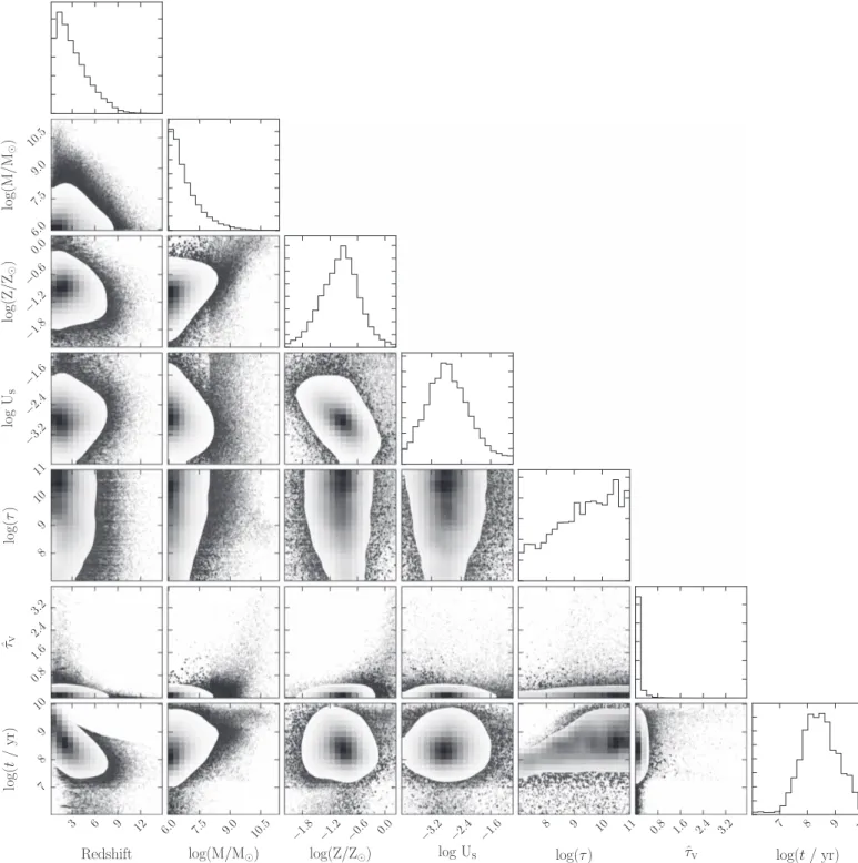
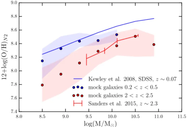
log S, which sets the ratio of H-ionizing photons to H atoms at the edge of the Strömgren sphere, the interstellar metallicity ZISM, and the dust-to-metal(mass) ratiox , which traces metald depletion onto dust grains. Since the gas density nH and depletion factor x do not significantly affect emission lined ratios at sub-solar metallicities(see Figures 3 and 5 of Gutkin et al. 2016), and most of our galaxies exhibit log(Z Z)
0.5
- (see Figure12), we fix nH=10 cm2 -3, the typical value measured in z~ – galaxies2 3 (e.g., Sanders et al.2016; Strom et al.2017), andx =d 0.3, a value similar to that measured in the Solar neighborhood (although, see Section 6.5). We account for attenuation by dust of the emission from stars and photoionized gas using the two-component model of Charlot & Fall (2000), parametrized in terms of the total attenuation optical depthtˆ , and the fraction of this arising inV the diffuse ISMμ. The mean effects of intergalactic medium absorption are included following the model of Inoue et al.(2014).
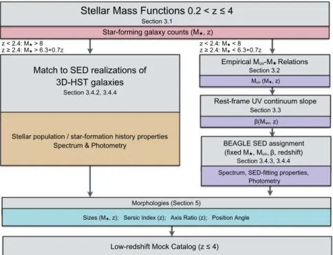
Figure 1.Diagram summarizing the procedures for generating star-forming galaxies at z . M4 is defined aslog(M M). High-mass galaxies(defined as M>8
for z<2.4 and M>6.3+0.7zfor z2.4;illustrated by the left pathway) and low-mass galaxies (right pathway) are generated differently as indicated. These criteria are defined in Section3.4.4as the approximate mass completeness limits in the 3D-HST catalog, which we use to assign real galaxy SEDs to high-mass mock galaxies. Gray boxes indicate the empirical relationships, distributions, or data on which mock galaxy properties are based, and colored boxes indicate the mock galaxy property generated in that step. Quiescent galaxies are generated at z<4 following a different procedure, which is described in Section4and illustrated in Figure13.
For mock galaxies with properties that are observable using current facilities, we use BEAGLEto generate a distribution of model SEDs consistent with the observations and assign these SEDs to the mock objects. To achieve this, wefit SED models fromBEAGLEto the multi-band photometry of galaxies in two CANDELS fields using the 3D-HST catalog (Skelton et al. 2014). When performing parameter estimation, BEAGLE
employs the nested sampling algorithm (Skilling 2006) as implemented inMULTINEST(Feroz et al.2009). This procedure creates a range of statistically acceptable SED fits for each observed galaxy in a subset of the 3D-HST sources (see Sections 3.4.2and 4.2, while for more detail of the BEAGLE
output, seeC16, Section3.3), which are then used to produce a parent catalog. This parent catalog is used to assign SEDs to mock objects with high stellar mass (i.e., those with mass abovelog(M M)>8, or above the mass completeness of the 3D-HST catalog if larger in that redshift bin) and low redshift (z<4), where the l4.5 mm photometry provides firm constraints on stellar mass. The SEDs are assigned by finding the closest match in stellar mass and redshift for each mock galaxy within the parent catalog, allowing us to encapsulate the observed diversity of galaxy SEDs at z<4 with relatively few assumptions.
For mock galaxies with realized properties that extend beyond current measurements of real sources, we can leverage the capabilities of BEAGLE to produce theoretical SEDs and generate model spectra for the mock objects. In this second method, we generate a parent catalog built of theoretical SEDs covering a range of model parameters that can be matched to mock galaxy stellar mass, redshift, and, for star-forming galaxies, MUV, and β (see Sections 3.4.3 and 4.2). We use this method at low stellar masses [log(M M)<8], where current galaxy survey sampling of the population is less complete, and at z , where SED coverage in the rest-frame4
optical is only available from imaging taken with IRAC, the 3.6–8 μm camera on Spitzer (Fazio et al.2004).
3. Generating Star-forming Galaxies across Cosmic Time Here we describe the phenomenological model and quanti-tative procedure for generating counts, redshifts, stellar masses, luminosities, and photometric and spectroscopic properties for mock star-forming galaxies. Galaxies are assigned masses and redshifts according to evolving stellar mass functions, as described in Section 3.1. In Sections 3.2and 3.3we describe the procedure for assigning integrated star-forming galaxy properties (MUV and β) based on empirical distributions. Finally, in Section3.4, we describe the procedure for assigning SEDs to star-forming galaxies.
3.1. Generating Star-forming Galaxy Counts
In generating a mock galaxy catalog, we aim to reproduce measurements of the star-forming galaxy stellar mass functions at low redshift(z4) and the UV luminosity function at high redshift(z4). Our primary mass function constraints come from Tomczak et al. (2014, hereafter T14), while our UV luminosity function constraints are adopted from Bouwens et al. (2015) at 4 z 8 and the newest z∼10 estimate presented in Oesch et al.(2017).
T14 provide measurements of the stellar mass function of star-forming and quiescent galaxies in eight redshift bins in the range 0.2< < . They employed imaging data from thez 3 FourStar galaxy evolution (ZFOURGE) survey (Straatman et al. 2016) covering the CDFS, COSMOS, and UDS fields withfive near-IR medium-bandwidth filters spanning the J and H bands, as well as broad-band KSimaging. Specifically they used the regions that also overlap with CANDELS J125 and H160imaging(to ∼26.5 depth to 5σ), covering a total area of ∼316 arcmin2. Additionally, imaging from NEWFIRM Figure 2.Diagram summarizing the procedures for generating the star-forming galaxies at z4. Mis defined aslog(M M). Gray boxes indicate the empirical
relationships, distributions, or data on which mock galaxy properties are based, and colored boxes indicate the mock galaxy property generated in that step. All star-forming mock galaxies at z>4 are generated following these procedures. Quiescent galaxies are generated at z>4 following a different procedure, which is described in Section4and illustrated in Figure13.
Medium-band Survey (Whitaker et al. 2011) was used in the AEGIS and COSMOSfields, employing the same filter sets as the ZFOURGE survey to shallower depths but wider area to leverage better constraints of the high-mass end of the mass function. Each of the fields also benefit from further imaging that allows comprehensive sampling of galaxy SEDs over the wavelength range 0.3–8 μm, with the field-specific filter sets and imaging programs summarized in Section 2.4 of Straatman et al.(2016).
T14 inferred photometric redshifts and rest-frame colors (used to separate galaxies into star-forming or quiescent based on the UVJ diagram of Whitaker et al. 2011) using the template-basedEAZYcode(Brammer et al.2008), while stellar masses were estimated usingFAST(Kriek et al.2009). Within
FAST, they used the original Bruzual & Charlot (2003) population synthesis code atfixed solar metallicity, employing a Chabrier (2003) IMF, and a declining exponential star formation history. The 80% mass completeness limits of their sample increase from log(M M)~7.75 at z∼0.5 to
M M
log( )~9.25 at z∼3. T14 fit their resulting stellar mass functions with a sum of two Schechter (1976) functions:
M dM M dM M dM dM dM ln 10 10 exp 10 ln 10 10 exp 10 , 4 M M M M M M M M 1 2 1, 1 2, 1 M M 1,M 1,M 1,M 2,M 2,M 2,M * * * * * * f f F = F + F = ´ -+ ´ -a a - + -- + -( ) ( ) ( ) ( ) ( ) ( ) ( )( ) ( )( )
where M=log(M M), as defined in Section 2.1, F(M) indicates the number of galaxies per Mpc3with stellar masses between M and M+dM, and M1,* , MM 2,* ,M f ,1,*M f ,*2,M a ,1,M
and a2,M are the six free parameters of the function.
19
In a single Schechter function, MM* is the mass at the turnover, or “knee” of the mass function;f is the characteristic number*M density of galaxies at the turnover; and a is the low-massM slope. In the double-Schechter function used in T14, they explicitly set M1,*M =M2,*M=MM*, meaning that theyfit with a single “knee” but the different normalizations and faint-end slopes of each function enable them to fit the observed steepening of the mass function to low masses (see Figure4). At z>4 stellar masses become progressively less well constrained from measurements, in part because the rest-frame optical SED (a key region containing the Balmer break at ∼3600 Å, and the 4000 Å break) shifts into the infrared where current facilities have low sensitivity. Additionally, high equivalent width (EW) emission lines can add to the flux in the reddest photometric bands, leading to an overprediction of galaxy stellar masses(Schaerer & de Barros2010; Curtis-Lake et al.2013; Stark et al.2013; de Barros et al.2014). As a result, relative uncertainties on stellar mass measurements are high (e.g., 0.4 dex at1010M
at z= 4, increasing with redshift and decreasing mass; Grazian et al. 2015; see also Mobasher et al. 2015) and may contribute to the large scatter of mass function measurements in the literature (nearly ∼1 dex in counts; see Figure 9 in Song et al. 2016, and Figure 11 in Davidzon et al.2017). Therefore, to generate galaxy counts at z>4, we leverage the constraints provided by the observed
UV luminosity function in the range of 4 z 8 from Bouwens et al.(2015) with luminosity function measurements with mean redshifts at zá ñ = [3.8, 4.9, 5.9, 6.8, 7.9] using data from the HST Legacy Fields, as well as the z∼10 luminosity function of Oesch et al. (2017). The binned UV luminosity function measurements we use for this work are overall consistent with many other results in the literature at MUV<−17 (e.g., McLure et al. 2013; Atek et al. 2015; Finkelstein et al.2015; Laporte et al. 2015; Castellano et al. 2016; Bouwens et al. 2017b; Livermore et al. 2017; Ono et al.2018; Yue et al.2017).
We choose to model the redshift evolution of the six mass function parameters across the entire redshift range of the mock (i.e., 0.2< <z 15). This ensures a smooth evolution in number counts across the transition from mass to luminosity function-based constraints. At z<3.8 (the mean redshift of the B-dropout sample used to produce the Bouwens et al. (2015) z∼4 luminosity function), we use the measured mass functions ofT14to directly constrain their redshift evolution, while at z3.8 we use our model of the redshift-evolving MUV–M relation (see Section 3.2) to fit to the observed luminosity functions with mass function parameters. However, it is important to note that this is not a direct prediction of the shape or evolution of the z4 mass functions that we expect to measure with JWST. Our z4 mass functions are dependent on our model of the MUV–M relation, and additionally we do not yet know how incomplete the current MUV-selected samples at z4 may be.
To determine a suitable form for the redshift evolution of the Schechter function parameters, we first need to know what mass function parameters can reproduce the observed UV luminosity functions at z4. The details of this fitting are given in Appendix A.1, and we plot the Schechter (mass) function parameters that bestfit the z4 luminosity function observations in Figure 3, as well as the individual maximum-likelihood estimates of T14 at z<4. The estimates of MM* derived from the measured luminosity functions at z 4 are significantly lower than theT14measurements. However, if we fit the evolution of a double-Schechter function with different “knees,” as in Equation (4), we can use M1,* to fit to the high-M mass end of the z<3 mass functions, while M2,* (plus the fastM evolution of 1,
M
*
f ) can be used to account for the rapid evolution in the bright end required to fit to the z4 luminosity functions. We therefore choose to set the z3.8evolution of M2,* ,M a , and2,M f*2,M using a weighted least-squares linear
regression to the luminosity function fits. We extrapolate the linear fit of M2,* to z<3.8 but re-fit theM T14measured mass functions, allowing the other five Schechter function para-meters to vary. In fact, this choice of M2,* evolution somewhatM under-estimates the high-mass end of the 2< <z 3 mass functions(see Figure 4). It is entirely possible that the reason for the strong evolution in MM* seen between the z<3.8 and z3.8samples is due to the MUV-selected samples missing a population of dusty, high-mass star-forming galaxies. If they exist, these objects will be revealed by JWST, but currently we lackfirm constraints on their number density evolution. We are basing this mock catalog on current observational constraints, and so choose to favor thefit to the z∼4 luminosity function over the2 mass function at the high-mass end, as itz 3 allows us to produce a model with number counts that vary relatively smoothly with redshift. As such, a caveat of our model is that we are not modeling the dusty star-forming
19
Schechter function parameters used to describe a mass function are suffixed by an “M” to distinguish them from those used to describe a luminosity function.
galaxies currently missed in UV-selected samples, and mildly under-represent the high-mass end of the 2 z 3 mass functions. A model that simultaneouslyfits the z∼2.75 T14 data and the z∼4 Bouwens et al. (2015) luminosity function would require a strong gradient discontinuity in M1,* thatM would lead to a step discontinuity in the number counts of galaxies at high stellar masses.
When fixing the evolution of the Schechter function parameters at z4, we use a weighted least-squares linear regression excluding the point at z∼10, which has noticeably lower number densities than can be accounted for by a simple linear relation in all three parameters. In fact, the exact form of the redshift evolution of the UV luminosity function, and associated CSFRD above z∼8, has been an area of active debate in the literature—for example, with McLeod et al. (2016) presenting measurements of the z∼9–10 luminosity function that are consistent with a smooth decline in the CSFRD. For ourfiducial mock catalog we choose to base the model on the Oesch et al.(2017) results in order to provide a conservative limit on z8 galaxy number counts likely to be detected with JWST. We defer further discussion of this issue to Section 7. The constraints at z∼10 are not strong enough to constrain the likely evolution in M2,* ,M 2,
M
*
f anda . We thus2,M
choose to re-fit the z∼10 luminosity function witha2,M and M2,* fixed to the values defined by the extrapolated linear fits atM z= 10, giving log 2, Mpc dex3 1 4.67 0.3
M
*
f - = -
( ) . We then
require the gradient of the evolution in log(f*2,M) to decrease further at z>8, so that this value is reached by the relation at z= 10.
At z<3.8 we re-fit to the T14 mass functions using a Bayesian multi-level modeling approach (see Appendix A.2), which allows us to derive the best-fit redshift evolution of the Schechter function parameters by fitting to the mass function measurements in each redshift bin simultaneously. This approach is more powerful than fitting a functional form to the published Schechter parameter estimates, as it accounts for parameter covariance self-consistently. At z<3.8, we choose a functional form for the redshift evolution fora2,M andf*2,M
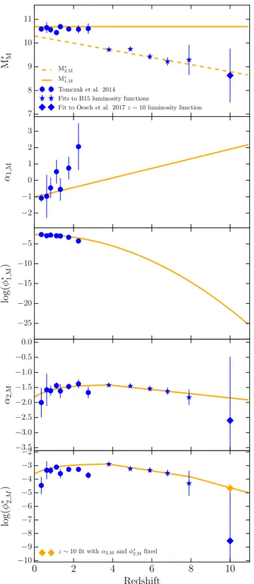
Figure 3. Redshift evolution of each parameter of the double-Schechter function adopted in our model. The orange lines show the adopted evolution, while circles represent the original maximum-likelihood estimates fromT14, with M1,*M=M2,*M set explicitly in the fitting. Stars (diamonds) show the median 68% confidence intervals for the parameter estimates from our MCMC fitting (described in Appendix A.1) to the Bouwens et al. (2015) luminosity functions at z∼4, 5, 6, 7, and 8 (Oesch et al.2017z∼ 10; see text for details). The orange diamond in the lowest panel shows the z∼10 luminosity functionfit when fixing the values ofa2,Mand MM*. The errors on
the z∼10 estimates are symmetric, so we choose to reduce the y-axis range of the panels displaying the redshift evolution of a2,M and log(f*2,M) for clarity.
Figure 4. Evolution of the star-forming galaxy mass function from z
0.2< <8.0 (lines), plotted with the observations fromT14(circles). The parameters of thisfit to the MF evolution are given in Equations (5)–(10) and Table4.
that asymptotically approaches the value of the best-fit linear relation at z= 3.8, but decreases rapidly at the lowest redshifts. Without this dip to low redshifts, the mass function is too shallow, with too high a normalization at low masses. We accept a mildly discontinuous evolution at z= 3.8 because allowing the functional form in eithera2,M orf2,*M to increase
and turn over by z= 3.8 (to give smooth evolution at z = 3.8) produces mass functions that cross over at low masses, a situation that we are trying to avoid by requiring that our model is monotonically increasing at given mass with decreasing redshift.
The redshift evolution of each Schechter function parameter is summarized below: M1,*M( )z =a1 ( )5 z b b z b z log[f1,*M( )]= 1+ 2 + 3 2 ( )6 z c c z 7 1,M 1 2 a ( )= + ( ) M2,*M( )z =D1+D z2 ( )8 z e z e z E E z z E E z z log 1 exp 3.8 3.8 8 8 9 2, 1 2 1 2 1 2 M * f = - - + < = + < = ¢ + ¢ [ ( )] [ ( )] ( ) 10 z f z f z F F zz 1 exp 3.8 3.8, 2, 1 2 1 2 M a = - - + < = + ( ) ( ) [ ( )]
where the parameters D1, D2, E1, E2, F1, and F2 are all determined from the linear regression to the forward-modeled luminosity functionfitting, and E1¢ and E2¢ are chosen to fit to the z∼10 luminosity function while maintaining continuous evolution in log[f ( )] at z = 8. The parameters e*2,Mz 2and f2are fixed to the values required to produce continuous evolution at z= 3.8 with e2=E1+3.8E2-e1[1 -exp(-3.8)] and f2 = F1+3.8F2-f1[1-exp(-3.8)]. The remaining free para-meters a1, b1, b2, b3, c1, c2, e1, and f1, are then constrained
using multi-level modeling (see Appendix A.2) to the publishedT14star-forming mass functions(their Table 1).
We report the median values and associated uncertainties, along with the values for the model parameters defined by linear fits to the z4 individual mass function estimates in Table 4. The chosen redshift evolution of each parameter is plotted as the orange lines in Figure 3. The resulting mass function comparisons to the T14 measurements at z<4 are plotted in Figure 4, and the luminosity function comparisons are shown in Figure5.
3.2. The Evolution of the MUV–M Relation
In this section, we describe our method to characterize the relation (slope, intercept, scatter) between MUV and M of galaxies at redshifts 0.2 z 15. Hereafter, we use the definition of MUV adopted, for example, in Robertson et al. (2013), as the average magnitude at rest-frame wavelength within a flat filter centered at 1500 Å and with a width of 100Å, which is the definition adopted byBEAGLE(Chevallard
& Charlot2016). This definition of MUV differs slightly from that used to measure the UV luminosity functions in Bouwens et al.(2015), which define MUVto be at rest-frame wavelength of 1600Å. We calculate the typical color correction based on the mean β as a function of MUV and redshift presented in Bouwens et al. (2014) and find that the typical difference in magnitudes between 1500 and 1600Å is negligible ( M∣d UV∣0.05). This correction is significantly smaller than the k-correction applied to estimate MUVat 1600Å from broad-band photometry in thefirst place ( M∣d UV∣0.1), and so we apply no conversion between rest-frame 1500 and 1600Å MUV values.
The MUV–M distribution and its evolution are critical components of our underlying phenomenological model, and are required to statistically assign UV luminosities to mock galaxies generated from our continuously evolving stellar mass function model. However, we note the following uncertainties Table 1
The Values of the Parameters Used in Our Model of the Mass Function Evolution, as Described in Equations(5)–(10)
Parameter Median 1σ Uncertainty Prior/Source of Fits
a1 10.69 0.04 (0, 50) b1 −2.68 0.16 (0, 50) b2 0.06 0.24 (0, 50) b3 −0.19 0.08 (0, 50),Î -¥[ , 0] c1 −1.02 0.16 (0, 50) c2 0.29 0.13 (0, 50) D1 10.30 0.10 Linearfitting 4z<8 D2 −0.15 0.02 Linearfitting 4z<8 e1 0.73 0.26 (0, 50),Î[0,¥] e2 −3.60 L = +E1 3.8E2-e1[1-exp(-3.8)] E1 −2.03 0.41 Linearfitting 4z<8 E2 −0.23 0.09 Linearfitting 4z<8 E1¢ −0.67 L f*2,Mfit to z∼10 LF E2¢ −0.40 L f*2,Mfit to z∼10 LF f1 0.41 0.17 (0, 50),Î[0,¥] f2 −1.82 L = +F1 3.8F2-f1[1-exp(-3.8)] F1 −1.16 0.10 Linearfitting 4z<8 F2 −0.07 0.02 Linearfitting 4z<8
Note.For those parameters determined using the multi-level modelfitting to z<4 mass functions, we report the median of the posterior distribution function, its 1σ confidence interval, as well as the prior used in the fitting.
to this procedure. At all redshifts, galaxies exhibit a diversity of mass-to-light ratios, which depend on the stellar population properties (age, metallicity), star formation history, and dust content of a galaxy. As a result, the exact form of the relation between MUVand Mand its dependency on galaxy properties are largely unknown. In general, brighter galaxies at UV wavelengths correspond to more massive objects (e.g., Stark et al. 2009; González et al.2011; Lee et al. 2011), and this holds out to z∼7 (Duncan et al. 2014; Grazian et al. 2015; Salmon et al. 2015; Song et al. 2016). Although the relation between MUV and M follows a general trend of decreasing MUV with M out to log(M M)~10, at higher masses the average MUV becomes fainter due to the appearance of a population of fainter objects. This trend could be attributable to several effects, such as increased dust content and older average stellar ages among massive galaxies(e.g., Spitler et al. 2014). Characterizing the relationship is further complicated by the difficulty of measuring stellar mass owing to emission line contamination at high redshift (Labbé et al. 2013; Stark et al. 2013) and at low stellar masses (Whitaker et al. 2014), and the lack of a direct photometric probe of MUV at intermediate redshifts (0.6< <z 1.5). The procedure we outline here has a direct impact on the resulting UV luminosity functions (see Sections 2.1, 3.1, and 6.1). We have therefore developed a straightforward description of the MUV–M distribution and its evolution that is designed to encapsulate the diversity of real galaxies.
3.2.1. Characterizing the Evolution of MUV–Mfrom Observations We characterize the MUV–M relationship at z4 using measurements from the 3D-HST catalog (using SED fitting with BEAGLE; see description in Section3.4.1). As discussed extensively in Stefanon et al. (2017a), selection effects can heavily influence the observed shape of the MUV–M distribu-tion. Therefore we avoid including observed galaxies whose MUV or M measurements are poorly constrained by the
BEAGLE fits. Specifically we only use galaxies with
M M
log 1
d ( )< , zd < , and M1 d UV<1 (where, e.g., zd is
the 68% credibility interval on redshift). The limits imposed were chosen to avoid biasing the characterization of the MUV–Mdistribution with overly strict MUVor Mcuts, which we discuss further below.
In Figure 6, we plot the MUV–M distributions for the 3D-HST galaxies with well-constrained MUV, M, and redshift measurements. As discussed above, these distributions show a trend of increasing stellar mass with decreasing MUV at low stellar mass. At high stellar mass the MUV values tend to be fainter than the linear relation, as observed in Spitler et al. (2014). Rather than attempting to fully model this mass-dependent behavior, especially given the Malmquist biases that begin to affect the higher-redshift bins, we adopt the following two-step procedure to describe the MUV–M distributions at z4. We fit the observed MUV–M distribution under the simplest assumption of a linear relationship to extrapolate to low masses, while at higher masses (log(M M)8–8.5, depending on the mass limit at a given redshift), we assign MUV values by sampling from real galaxies of the same mass. The matching procedure allows us to maintain the observed flattening of the distribution at high masses, and is fully described in Section3.4.2below.
Figure 6 illustrates the substantial scatter in the observed MUV–Mdistributions at z4. Owing to the large scatter, the best-fitting slope will depend strongly on the uncertainties on the data points, and the size of the uncertainties may depend on MUV, M, and also plausibly on redshift. Indeed, we find that when fitting with both slope and normalization as free parameters, neither parameter is well constrained, and the best-fitting slope is highly variable between redshift bins. Therefore we adopt afixed slope for the MUV–Mrelation at all redshifts and fit only the intercept at each redshift. This procedure essentiallyfits the average redshift-dependent mass to light ratio, which has lower uncertainty and is less dependent on the error on individual galaxy measurements and stellar mass-dependent systematics. Several studies have reported the measurement of constant slope for UV-selected galaxies, with normalization evolving in redshift(Duncan et al.2014; Grazian et al. 2015; Salmon et al. 2015; Song et al. 2016; Stefanon et al.2017a), and find a reasonable description of the data. The blue dashed line in Figure6 shows our best-fit relation to the MUV–M distribution in each redshift bin, where the slope is fixed to a value of −1.66. We find excellent agreement with the observed distribution at all redshifts. For reference we also indicate the stellar mass limits in each redshift bin, above which we assign MUV values by sampling from real galaxies (red dashed lines). Fitting the MUV–M distribution only above these mass limits instead has a negligible effect on the result at z<3. At z∼3.75, where there are fewer well-constrained measurements,fitting above this mass limit would increase the MUV–Mintercept by∼0.1 mag, an indication that fitting only at the high-mass end biases the characterization of the MUV–M due to the high-mass end flattening. Therefore we choose to proceed using all galaxies with well-characterized stellar mass, redshift, and MUV.
To set the full redshift evolution of the MUV–Mrelation, we combine the intercept values for the best-fit relations with fixed slope at each redshift z4, with measurements of the MUV–M intercept at z>4. We use the average observed value of stellar mass for bright (MUV=−20) galaxies at
z
4< 7 to set the overall normalization in each z>4 redshift bin, while assuming the same constant MUV–Mslope. Figure 5. UV luminosity function at z4 of our continuously evolving
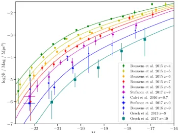
phenomenological model(solid lines; described in Section3), evaluated at the mean redshift of the dropout samples used in thefitting. Points are observations at the same mean redshifts as indicated by the colors(Oesch et al.2013,2017; Bouwens et al.2015,2016b; Calvi et al.2016; Stefanon et al.2017b). Our forward modeling approach explicitly fits to the binned UV luminosity functions of Bouwens et al.(2015) and Oesch et al. (2017).
Figure 6. MUV–Mrelation for realizations drawn from the SEDfits to observed star-forming galaxies (log sSFR( )< -10Gyr−1) in the 3D-HST survey (blue points) with high-confidence measurements of MUV, M, and redshift, as described in Sections3.2and3.4.1. Blue dashed lines indicate the best-fitting linear relationship under
the assumption of afixed slope, as described in the text. Solid black lines indicate the smoothly evolving redshift-evolution of the MUV–Mrelation in our model, as
characterized in Figure7and Equation(11). The red dashed line indicates the stellar mass above which mock galaxies are matched to 3D-HST realizations, which is the larger betweenlog(M M)>8andlog(M M)>6.3+0.7z(the evolving mass limit exceedslog(M M)>8at z>2.4).
We utilize the high-redshift stellar mass measurements shown in Figure 7 of Stark et al. (2013), where the measured stellar masses were fit while including the contribution to the SED from nebular emission lines. The normalization value at MUV= -20 shows an overall decline in the range of
z
4 < , indicating a decrease in the average mass to light7 ratios of galaxies with increasing redshift. The measured values for the MUV–M intercepts at all redshift bins, evaluated at MUV= - , are shown as points in Figure20 7.
3.2.2. Continuous Redshift Evolution of MUV–M
Our model of the redshift evolution of the MUV–M relation is defined by fitting to the evolving intercept values shown in Figure7. These intercepts show a rapid decline from z∼0–3, with a shallower decline at z>4. We find that at z 4 the intercept measurements are adequately described by a quadratic function, and a linear function at z>4. To ensure these two functions remain continuous at z∼4, we include the boundary condition that the derivatives of the two functions are equal at the center of the highest redshift bin where we use the 3D-HST data(z = 3.75). This constraint results in the following function to describe the intercept of the MUV–M relation, MM0UV–M( )z, evaluated at MUV= -20 and z3.75: M z a z b a z z c 3.75 2 3.75 3.75 , 11 M M 0 2 UV = -+ - - - + ( ) ( ) [ ( )] ( ) ( ) –
where a= 0.12, b = 0.08, and c = 9.41. This evolution of the MUV–M intercept is shown as the black solid curve in Figure 7, along with the observed data (blue points). The resulting linear MUV–M relations in each redshift bin, according to the smoothly evolving intercept function defined in Equation (11), are also shown as black solid lines in Figure 6. At z>3.75, the MUV–M intercept evaluated at MUV= -20evolves approximately linearly with the following
form: M z z M z 3.75 8 0.12 9.88 8 8.92. 12 M M M M 0 0 UV UV < < = - ´ + = ( ) ( ) ( ) – –
We use Equation(11) to assign MUV values to galaxies of a given stellar mass and redshift at z3.75, and Equation(12) to assign MUV values at z>3.75, assigned randomly within the scatter observed in 3D-HST data in Figure 6. We have characterized this scatter in both stellar mass, MUV, and redshift, andfind that the scatter in MUVis remarkably constant in both stellar mass and redshift, with an average value of
0.7 uv
s ~ magnitudes. Therefore, at all redshifts, we assign MUV values randomly according to this relation and that assumed Gaussian scatters . This direct assignment of Muv UV applies only to low-redshift low-mass star-forming mock galaxies (z4 and have log(M M)8), or high-redshift star-forming galaxies at z>4. Massive, low-redshift mock galaxies (withlog(M M)>8 and z ) are assigned MUV4 values according to their matched 3D-HST realization. The MUV–M relation and scatter, as described here, are used as priors when drawing realizations fromfits to 3D-HST galaxies to ensure a smooth transition in the mock catalog MUV–M relation at log(M M)=8. This procedure is detailed in Section3.4.2.
3.2.3. Theoretical Limits on the Mass to Light Ratios of Galaxies As mass to light ratios continue to decrease with increasing redshift and decreasing stellar mass according to our model, the mass to light ratios approach a theoretical limit of the stellar population models we generate withBEAGLE. This limit is set by the UV luminosities of individual massive stars, and represents the minimum mass to light ratio possible for an instantaneous burst of star formation for any given IMF(with no dust attenuation, the lowest metallicity, and corresponding nebular continuum emission). Any IMF choice will result in such a limit in the possible MUVgiven a stellar mass, with more top-heavy or bottom-light IMFs allowing for brighter limiting MUV and bottom-heavy IMFs producing fainter limiting MUV. The Chabrier IMF that we use in this work is relatively bottom-light and has a larger mass to bottom-light ratio parameter space than a more bottom heavy IMF (e.g., Salpeter 1955; Kroupa 2001). For a Chabrier IMF with our assumed high-mass cutoff of 100 M, we find that the stellar plus nebular continuum emission results in a theoretical mass to light ratio given by MUV» -2.45 log(M M)-1.3.
To accommodate this theoretical limit in the MUV–M evolution of our phenomenological model, we truncate the Gaussian distribution that we use to assign MUV values. For galaxies at the detection limit of future blank surveys (e.g., apparent magnitude mapp~31) this truncation has a negligible effect on the overall MUV–M distribution at z<4. At z>4, we find that scatter using the truncated Gaussian at the limit changes the overall shape of the MUV–M distribution by steepening the low-mass end. The effect becomes significant by z∼8. We therefore additionally halt the redshift evolution of the mean MUV–M relation parametrized in Equation (12) at z= 8. A demonstration of theBEAGLEmass to light ratio limit is shown in Figure8, compared with the projected evolution of the mean MUV–M relation allowed to evolve past z∼8.
Although we make every effort to choose reasonable constraints where available, the overall shape of the MUV–M Figure 7.The redshift evolution of the intercept of the MUV–Mdistribution,
MUV0 -M( ), dez fined at MUV= - . Blue points indicate the best-fit intercept20
to the 3D-HST data presented in Figure6, assuming afixed slope. Error bars are smaller than the size of the symbol. Orange points are based on the relation presented in Stark et al.(2013) that includes the correction for nebular emission lines.
distribution at z>4 is still an extrapolation that impacts various evolutionary relations at high redshift in the model, including the UV luminosity function and sSFR. We will discuss these issues in depth in Section6.
3.3. UV Continuum Slope–MUV Relationship
The spectral slope of the UV continuum(β where fl µlb) of galaxies is sensitive to the properties of stellar populations(e.g., metallicity and age), star formation history, and dust attenuation. Population studies of star-forming galaxies indicate well-characterized relationships between β and UV luminosity. Bright, massive galaxies tend to have red (i.e., shallower) UV continua, which likely owes to a combination of old stars, higher stellar metallicities, and a larger dust content. The bluer (i.e., steeper) UV continua of lower luminosity galaxies are often associated with younger, less metal-rich stellar populations, and less dust attenuation (e.g., Stanway et al. 2005; Labbé et al. 2007,2010; Bouwens et al.2009, 2012b; Rogers et al. 2013, 2014). The detailed relations between β and MUV, scatter, and evolution out to redshift z∼8 are still areas of active research, but many studies are consistent with a linear relationship betweenβ and MUV (e.g., Bouwens et al. 2012b, 2014; Alavi et al.2014; Kurczynski et al.2014; Rogers et al.2014) with an average evolutionary trend toward bluer β with increasing redshift(e.g., Labbé et al. 2007; Bouwens et al. 2009; Wilkins et al. 2011; Castellano et al. 2012; Finkelstein et al. 2012b; Bouwens et al.2014).
3.3.1. Meanb–MUVRelation across Cosmic Time
We use a compilation of measuredβ–MUVrelations and their scatter across redshifts to assign the rest-frame UV SEDs of mock galaxies. Following several studies (see the previous section), we model the average β–MUV relation with a linear function, where the slope db ( )z dMUV and intercept
MUV 19.5,z
b( = - ) of the function vary with redshift. We
consider sets of β–MUV relations at1 z 8 obtained from HST/ACS (Alavi et al. 2014; Kurczynski et al.2014; Mehta
et al. 2017) and HST/WFC3 imaging (Bouwens et al. 2009, 2014). The relationships describing β–MUVat the high redshifts we model are broadly consistent with fits measured in other studies (e.g., Bouwens et al. 2012b; Rogers et al. 2014; Finkelstein et al.2015).
We find that the slope of the β–MUV relation shows little evolution at redshifts1 , as already found in previousz 8 works (e.g., Bouwens et al. 2012b, 2014; Kurczynski et al. 2014). The intercept of the relation increases significantly from redshift z∼1–8, reflecting the evolutionary trend that galaxies have older ages and higher metallicities at later cosmic times (e.g., Labbé et al.2007). We perform least-squares linear fits to measurements of both db ( )z dMUV and b(MUV= -19.5,z) and their errors from the literature to produce a mean relation that smoothly evolves with redshift(see Figure9), described by
d z dM z M z z 0.007 0.09 19.5, 0.09 1.49. 13 UV UV b b = - -= - = - -( ) ( ) ( )
For mock galaxies at z , we extrapolate this relationship to1 lower redshifts to assignβ values. At z>8 we use the β–MUV relationship at z= 8 to assign β to mock galaxies. There exist several motivations to curb the evolution of β–MUV, with the foremost being the existence of a theoretical limit on the steepness of the UV spectrum emitted by non-Pop. III stars(see discussion in Section3.3.2below). Further, the data do not yet constrain evolutionary trends at the highest redshifts currently accessible (z~ – ). While evolutionary trends with redshift5 8 are observed in most analyses (Finkelstein et al. 2012b; Bouwens et al. 2014), the combination of high-redshift color selections with flux boosting from noise in the filters used to measureβ are still likely causing statistical studies to be biased against redder β measurements at z>5 (Dunlop et al. 2012; Rogers et al. 2013). At the very highest redshifts currently accessible(z~ –7 10), the data do not provide strong evidence for or against any evolutionary trend inβ with redshift or MUV (Dunlop et al.2013; Wilkins et al.2016), although the dynamic range in MUV is relatively small at such early times. While evolution cannot be excluded by current data, deep imaging Figure 8.Demonstration of the evolution of the mean MUV–Mrelation with
redshift (if mass to light ratios were allowed to continue decreasing above z>8) in comparison to the mass-to-light ratio limit imposed by the stellar population modeling withBEAGLE(which implicitly assumes a Chabrier IMF with a high-mass cutoff of 100 M). In our model, all z>8 galaxies follow the
MUV–M relation at z= 8 to avoid a scenario where significant numbers of
galaxies exceed the theoretical mass-to-light ratio limit set byBEAGLE.
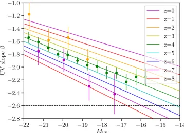
Figure 9.Redshift evolution of the meanβ–MUVrelation. Intrinsic scatter is
included as described in Section3.3.3. Points indicate a selection of binned measurements from(Bouwens et al.2009,2014, circles) at similar redshifts of the colored lines(orange at z∼2.5; green at z∼4; magenta at z∼7). The black dashed line indicates the theoretical limit in the BEAGLE models as discussed in Section3.3.2.
surveys with JWST will enable more robust characterization of the evolution beyond z∼8.
In our model, all mock galaxies are assigned aβ according to the mean relationship and intrinsic, photometric bias-corrected scatter described in Section3.3.3. We now detail the theoretical predictions for the UV continuum slope of our combined stellar population and photoionization model.
3.3.2. Theoretical Limits on UV Continuum Slopes Model predictions on the shape of the UV continuum emission of galaxies depend on the assumed properties of stellar populations and ISM (gas and dust). Young, massive stars show blue UV continua, which become bluer with decreasing metallicity. The effects of stellar age and metallicity on the UV continuum emission over time in our spectral evolution model are illustrated in Figure10, which shows that the bluest UV spectra are obtained for very young ( 1 Myr) stellar populations with sub-solar metallicities (dashed lines). Dust reddens the emitted stellar spectrum, and leads to a relation between the attenuation suffered by a galaxy and its UV slope β (Meurer et al. 1999). Recombination-continuum from ionized hydrogen also reddens the UV continuum emission emerging from a galaxy. This effect is shown by the solid lines in Figure10, which illustrates how our combined stellar population + photoionization model predicts redder β slopes than a model accounting only for stellar emission.
In order to avoid unphysical values for the β slopes associated to our mock galaxies through the redshift-dependent β–MUV relation presented in Section3.3.1above, we impose a limit bmin= -2.6 for the bluest possible value. This limit corresponds, approximately, to the bluestβ value obtained with
BEAGLEfor a model with constant SFH, sub-solar metallicity, low depletion factor (x =d 0.1), and low ionization parameter (logUS= -3.5). We note that models with non-zero escape fraction of H-ionizing photons can reach bluer values.
3.3.3. Scatter in theb -MUVRelation across Cosmic Time The scatter in the β–MUV distribution discussed in Section3.3.1encodes the intrinsic diversity in age, metallicity, and dust attenuation of the galaxy population atfixed redshift and UV luminosity. We aim to assign β values to mock galaxies following the intrinsic scatter (i.e., corrected for photometric biases) of the β–MUV distributions over cosmic time. Much effort has been put into characterizing the scatter, and how it might change with redshift, UV luminosity, or other galaxy properties (e.g., Bouwens et al. 2012b). The intrinsic scatter inβ at fixed UV luminosity, σβ, is surprisingly uniform across all redshifts from z~ – , and relatively independent of1 6 UV luminosity with values in the range of s ~b 0.3 0.4– (Bouwens et al.2012b,2014; Kurczynski et al. 2014; Mehta et al. 2017). We note that there is some evidence for the intrinsic scatter of the distribution increasing with UV luminosity, such that populations of brighter galaxies will have larger intrinsic scatter in β (Rogers et al. 2014). This evidence comes from a careful analysis at z∼5 only, however, and such luminosity dependence in theσβis not characterized sufficiently across cosmic time to be incorporated in our model. We correspondingly adopt an intrinsic scatter ofσβ∼0.35 in our model uniformly across all redshifts and UV luminosities. To include intrinsic scatter σβ∼0.35 in our model, we assign β values to mock galaxies according to a Gaussian distribution with a mean defined at a given redshift and MUV according to Equation(13) with σβ= 0.35. To avoid values of β bluer than the theoretical limits described in the previous section(for which we would not be able to associate aBEAGLE
spectrum), we truncate the distribution at β = −2.6. With this truncated Gaussian scatter, at the very highest redshifts and faintest MUVthe mean value ofβ reddens slightly so as to cause a mild flattening of the linear relations shown in Figure 9. However, we accept this feature as more favorable than artificially fixing to the bluest value of β and reducing the galaxy diversity in the mock. In addition, it mimics the behavior of β–MUV seen in some studies that indicate an apparent flattening of the linear relation at faint luminosities (e.g., MUV -19; Bouwens et al. 2014). Future measure-ments from JWST imaging and spectroscopy will help inform our stellar population synthesis models as we uncover the full range and distribution of UV continuum slopes in the early universe.
As described further in the following section, when possible we use 3D-HST galaxies to provide the constraints on the shape of the SED for mock galaxies. However, when this is not possible, we use theβ slope that is assigned to each galaxy to match to a parent catalog of SEDs produced byBEAGLE(see
Section 3.4.3). This ensures that our catalog will follow observed trends inβ–MUV.
3.4. Assigning Galaxy SEDs and Spectroscopic Properties We assign a set of spectral properties to each mock galaxy, allowing us to provide filter photometry as well as a full spectrum for each object. The general method is to produce a parent catalog of spectra that can be matched to galaxies in the mock. Where possible we produce this parent catalog from the results of SED fitting to galaxies in the 3D-HST catalog, allowing the observed photometry to provide the diversity of observed SEDs at given stellar mass and redshift (see Section 2.3). We limit the use of these empirical SEDs to Figure 10. UV continuum slopes predicted by the spectral evolution model
adopted in this work. We show model predictions for a constant SFH of different ages and three metallicities:logZ Z= -2(blue), −1 (green), and 0 (orange). Dashed lines indicate predictions for stellar emission only, while solid lines for stellar and nebular continuum emission. In this latter case, we consider a photoionization model with ionization parameterlogUS= -2.5and depletion factorx =d 0.3.