Essays on financial markets and on effects of information and communication technology

E

SSAYS ON

F

INANCIAL MARKETS

AND ON EFFECTS OF

INFORMATION

&

COMMUNICATION TECHNOLOGY

PHD in TEORIA ECONOMICA E

ISTITUZIONI

XVII Ciclo

Stefania Di Giacomo

Relatori: Proff. Luigi Paganetto e

Università degli

studi di Roma

“Tor Vergata”

The first essay aims to implement the literature on stock market anomalies, by testing the performance of “value” and “growth” portfolio strategies formed on deviations between observed and discounted cash flow fundamental (DCF) values.

It presents evidence on the excess returns obtained when contrarian strategies are played on the basis of the above described more sophisticated trading strategies, which are reasonable proxies of the behaviour of “fundamentalist” traders.

The significance of “value” and “growth” strategies in different subperiods is adjusted for several risk measures including: i) covariance of portfolio returns with GDP growth; ii) exposition to systematic nondiversifiable risk; iii) exposition to additional risk factors (return’s skewness, small size and financial distress risk factors). About this last point, by combining Fama and French (1995) and Harvey and Siddique (2000) approaches, it extends the original one-factor CAPM to a four-factor CAPM model.

The results show that, both in the American (US) and European (EU) stock exchanges, “short term DCF value” strategies (based on a monthly selection of the stocks with the lowest observed to fundamental ratio in the previous period) have mean monthly returns which are higher than, not only the corresponding growth strategies, but also passive buy and hold strategies on the total sample portfolio (the benchmark).

Moreover they are not riskier in terms of covariance with GDP growth.

These results persist when returns are adjusted for risk, since risk adjusted intercepts of excess returns of value portfolios in four-factor CAPM estimates are still positive and significant.

The findings seem to suggest that semi-strong efficiency did not hold during the last 12 years. This is true for both EU and US sample, thus in the comparative evaluation of domestic financial systems the success of contrarian strategies seem not to be country specific and therefore not depending on specific features of different financial systems.

The second essay is dedicated to the study of how much “fundamental” and “non- fundamental” components matter in determining stock prices according to differences in regulatory environments and in the composition of financial market investors. A "two-stage growth" discounted cash flow (DCF) model, calibrated on the risk premium and on the terminal rate of growth, is built up to proxy the benchmark for the so called “fundamentalist” traders, while “non-fundamental” price components are interpreted as signals reducing asymmetric information (such as firm size, the number of earnings growth forecasts and the chartist momentum).

Empirical results on two samples of American (US) and European (EU) stocks show that the “fundamental” price earning ratio (P/E) explains a significant share of cross-sectional variation of the observed P/E. However, for US stocks (where there is more diffusion and transparency of information and more pervasive presence of pension funds, that may be expected to increase the share of long term investors adopting a fundamentalist perspective) the relationship between DCF fundamental and observed P/E is stronger than in the EU case.

It also documents that: i) the fundamental P/E has superior explanatory power with respect to simpler measures of expected earnings growth usually adopted in the literature and this for both samples; ii) the relevance of the “non-fundamental” components mitigates the role of the fundamentals; iii) only for the EU sample current deviations from the fundamentals are affected by ex post adjustment of publicly available information.

If we associate this last finding with that on the relatively different impact of fundamental values we find two pieces of evidence consistent with the Market Integrity Hypothesis (King and Roell, 1988; Bhattacharya and Daouk, 2000; Milia, 2000): reduced “insider trading” effects are generally related to higher reliance on fundamentals extracted from publicly available information.

Thus differences in regulatory environments and in the composition of investors between the US and EU financial systems may help to explain these comparative findings.

The third essay analyzes the contribution of Information & Communication Technology (ICT) to levels and growth of per capita GDP. In this perspective, it is

or by removing the “bottlenecks” which limit access to knowledge, with the effect of increasing the productivity of labour (see Quah, 1999).

Two different proxies are used in order to measure the technological factor: i) Chain-Weighted ICT1 index, which is composed by normalized data on telephone mainlines, on personal computers and on internet users; ii) Chain-Weighted ICT2 index, which is composed by normalized data on telephone mainlines, personal computer, internet users and by two different prices for internet access. These are internet provider access prices and internet telephone access prices ($ per 30 off-peak hours).

The econometric analysis compares the relative significance of the two hypotheses in level and growth estimates and find that, when separately taken, both hypotheses improve upon the classical Mankiw, Romer and Weil (1992)- Islam (1995) framework.

Moreover the Davidson-MacKinnon (1981, 1993) J-test for non-nested models shows the superiority of the first hypothesis when we use the ICT1 index (which includes ICT components which represent high-tech vintages of physical capital) and the superiority of the second hypothesis when we use the ICT2 index (more related to the bottleneck hypothesis, since it includes indicators of access prices).

Finally it is demonstrated that a mixed hypothesis which incorporates both dimensions of the ICT contribution to growth at the same time is preferred to the focus on only one dimension. The consistent improvement of “within” country significance in panel estimates documents that this approach captures two dimensions of time varying-country specific technological progress that previous standard approaches in the literature could not take into account.

Finally the forth essay is dedicated to the study of the role of technology (and, in recent times, especially of ICT technology) as a factor which, by affecting women’s empowerment and productivity, could have significant effects on fertility decisions.

To estimate the relationship between ICT and the fertility rates across different countries it is used a random coefficient model which takes into account model misspecifications, like omitted variables and heterogeneity.

The empirical results show that ICT diffusion has significant negative effect on fertility rates, after controlling for human capital and institutional quality.

Moreover this effect is highly heterogeneous across macroareas (five subgroups of countries are optimally identified) and the random coefficient method provides improvements with respect to the estimation approaches that assume homogeneous parameters (such as conventional OLS fixed effects, where the impact of ICT, measured in the aggregate, vanished). The incapacity of the seconds in finding significant effects for ICT on fertility rates depends from the impossibility of disentangling the general effect from some significant group specific deviations from it.

Furthermore, subgroup deviations from non random general parameters seem to be strongly affected by three latent factors: pro fertility religious norms of Catholic and Islamic culture, the degree of secularization and education of a country, and the digital divide.

In this sense, the variables measuring access to ICT seem to proxy the impact on fertility of openness to world highly secularized culture. Such impact is stronger in countries where ICT has a significant diffusion and where it seems to prevail over religious norms (Catholic and South Europe countries) while it is much weaker in low income countries suffering from the digital divide and in countries where religious norms are so strong to overcome the ICT openness effect.

Short term value strategies:

a comparative analysis in the US and EU markets

Leonardo Becchetti

University of Rome Tor Vergata, Department of Economics, Via di Tor Vergata snc, 00133 Roma.

E-Mail : becchetti@economia.uniroma2.it Stefania Di Giacomo

University of Rome Tor Vergata, Department of Economics, Via di Tor Vergata snc, 00133 Roma.

Abstract

The paper aims to implement the literature on stock market anomalies by testing the performance of “contrarian” portfolio strategies formed on deviations between observed and discounted cash flow fundamental (DCF) values in the US and European stock markets.

The significance of cross-sectional “short term DCF value strategies” in different subperiods is adjusted for several risk measures including: i) covariation of portfolio returns with GDP growth; ii) exposition to systematic nondiversifiable risk; iii) exposition to additional risk factors (return’s skewness, small size and financial distress risk factors).

Our findings show that, both in the US and EU stock exchanges, “short term DCF value strategies”: i) have mean monthly returns which are higher than, not only the corresponding growth strategies, but also passive buy and hold strategies on the total sample portfolio (the benchmark); ii) yield excess returns which are still significant after risk adjustment in 4-CAPM models; iii) are not riskier in terms of covariation with GDP growth. EU stocks have similar patterns when compared to US stocks in each of these features.

1. Introduction

The literature on explanatory variables of cross-sectional stock returns discusses the existence of size and book to market premia evaluating whether excess returns from portfolios of small size and low market to book stocks persist after risk adjustment.

While evidence on the existence of premia related to size and book to market factors is widespread (Lakonishok, Schleifer and Vishny, 1994; Clare, Smith and Thomas, 1997; Heston, Rouwenhort and Wessels, 1995, Bagella, Becchetti and Carpentieri, 2000), the discussion whether excess returns from these two variables are simply proxies of additional risk factors different from stock betas, or indicate the existence of market anomalies, is still open.

Some tentative explanations try to reconcile these cross-sectional findings with the Efficient Market Hypothesis. According to them size and book to market premia disappear once: i) multifactor CAPM (Fama-French, 1992, 1993 and 1996); ii) lead-lag relationships between large and small firm stocks (Lo and MacKinlay, 1990); iii) time-varying betas (Ball-Kothari, 1989) and iv) survivorship bias are properly taken into account.

A second group of papers rejects the validity of these interpretations and affirms that return premia on small size and low market to book stocks are too high and must be partially explained by investment strategies of noise (De Long et al., 1990), near rational (Wang, 1993), liquidity or “weak-hearted” traders

overreacting to shocks and extrapolating past stock price dynamics (Bagella et. al., 2000; Lakonishok, et al., 1994).1

More specifically, Lakonishok et al. (1994) and Haugen (1995) argue that the value premium in mean monthly returns arises because the market undervalues distressed stocks and overvalues growth stocks.

The limits of this literature are that theoretical arguments and the observed microstructure of contemporary financial markets are only loosely related. Furthermore, contrarian empirical tests consider strategies (such as those of building size, book to market, or past winners’ portfolios) which are relatively less sophisticated with respect to some of the observed strategies adopted by financial investors.

The marginal contribution of our paper goes in this last direction. We devise consistent “fundamentalist” investment strategies by building portfolios of value and growth stocks ordered on deviations between fundamentals2 _- calculated according to discounted cash flow (DCF) rules - and observed values. We therefore present evidence on the excess returns obtained when value strategies are played on the basis of the above described “more sophisticated” trading strategies which are reasonable proxies of the behaviour of fundamental traders.

Our paper is divided into five sections (including introduction and conclusions). In the second section we illustrate the methodology adopted for the

1 _{An agency cost related interpretation of this behaviour suggests that investment fund managers} may also be extrapolative as their choice of past winners may be easier to explain to sponsors (Lakonishok et al., 1994).

2 _{The evaluation of fundamentals is common practice in finance since an important school of} though bases its trading strategies on price deviations from fundamental values. An alternative approach is followed by the so called “chartists” which adopt trend-following strategies buying (selling) a rising (falling) stock even if it is above (below) the fundamental value predicted by the

estimation of the fundamental value of the stock. In the third section we provide descriptive evidence on mean monthly returns for value and growth portfolios. In the fourth section GMM three and four-CAPM estimates evaluate the profitability of “value” portfolio strategies formed on deviations between observed and fundamental stock values and test the stability of contrarian strategy premia in different subperiods.

2. Stock market anomalies: a synthetic reference to the state of art

The literature defines “stock market anomalies” return patterns which are not explained by the capital asset pricing model of Sharpe (1964) and Lintner (1965).

Well known stock market anomalies are: i) the reversal in long-term returns when stocks with low long-term past returns tend to have higher future returns (De Bondt and Thaler, 1985); ii) risk adjusted excess returns related to size, book-to-market equity, earning/price, cash flow/price and past sales growth (Basu 1983, Rosenberg, Reid and Lanstein 1985, Lakonishok, Shleifer and Vishny 1994, Bagella-Becchett and Carpentieri, 2001).

Fama and French (1993) argue that the anomalies disappear when adjusted for additional risk factors. Their 3-factor model implies that the expected return on a portfolio in excess of the risk-free rate [E(Ri)-Rf] is explained by the sensitivity of its return to three factors: i) the excess return on a broad market portfolio [Rm-Rf]; ii) the difference between the return on a portfolio of small size stocks and the return on a portfolio of large size stocks [SMB factor]; iii) the

difference between the return on a portfolio of high book-to-market value stocks and the return on a portfolio of low book-to-market value stocks [HML factor].

The expected excess return on portfolio p is:

t P t P t P f t m t P P f t P t HML E SMB E R R E R R E( )− =α +β [ ( )− ]+γ ( )+δ ( )+ε

The factor sensitivities or loadings, βP,γP,δP are the slopes in the

time-series regression t P t P t P f t m t P P f t P t HML SMB R R R R − =α +β ( − )+γ +δ +ε

If the three-factor model describes expected returns, the regression intercepts should not be significantly different from zero.

Fama and French (1992, 1993, 1995, 1996) find that their null hypothesis is not rejected since excess returns disappear when adjusted for the two additional risk factors. In contrast to them, other authors show in their empirical analysis that return premia on small size and low market to book stocks do not disappear and must be partially explained by investment strategies of noise (De Long et al., 1990), near rational (Wang, 1993), liquidity or “weak-hearted” traders overreacting to shocks and extrapolating past stock price dynamics (Bagella et. al., 2000; Lakonishok, et al., 1994).

A third intepretation of the existing empirical evidence considers contrarian strategy premia a spurious result for at least three reasons: i) they may be the result of data-snooping as the relevance of book to market and size factors may be sample specific; ii) they may be affected by a survivorship-bias given that the COMPUSTAT database gives excessive weight to distressed firms (with high book to market values) that survived rather than to distressed firms that failed; iii) OLS techniques used for estimating CAPM models are not robust with nonnormal

samples find that the significance of contrarian strategy premia is much lower when more robust GMM techniques, relying on weaker assumptions about residuals distribution, are adopted (MacKinlay and Richardson, 1991; Clare, Smith and Thomas, 1997).

In the next section we shift the debate into a new field by proposing a portfolio strategy which is more consistent with methods adopted by fundamentalists to calculate the fair value of the stocks. In this way we try to see whether fundamental contrarian strategies generate significant risk adjusted excess returns.

2. The simple DCF rule for portfolio selection

Accounting and economic literature usually adopt at least three different approaches to calculate the fundamental value of a stock: i) the comparison of balance sheet multiples (EBITDA, EBIT) for firms in the same sector; ii) the residual income method; iii) the discounted cash flow method.

The first approach has no rational grounds since, if market agents have nonhomogeneous information sets or adopt different trading strategies, the benchmark used for comparison may be overvalued or undervalued. A second problem is that, as far as firms diversify their activities and develop new products or services which cannot be easily classified into traditional taxonomies, industry classifications become tricky. Product diversification therefore makes it hard to assume that two firms classified into the same industry may have an identical

The problem with the second approach (residual income method) (Lee, et al., 1999; Frankel and Lee, 1998), is that the formula for evaluating the fundamental value of a stock uses a balance sheet measure whose accuracy and capacity of incorporating changes in the fundamental value of the stock is limited. A valuable example of this phenomenon is provided by Lee et al. (1999) who document the sharp uptrend in the price to book ratio which has risen three times between 1981 and 1996 for the Dow Jones Industrial Average. An interpretation for this result is that accounting methodologies lag behind in adjusting to changes in investors' market value assessments of firms whose share of intangible assets is changing over time. Moreover, book values tend to be seriously affected by historical or market value accounting choices on nonrealised capital gains/losses. This means that, depending on the rule adopted, the book value is not independent from market over or underevaluation.

This is the reason why, following Kaplan and Roeback (1995), we prefer to use the DCF approach. This approach is described also in previous contributions (Adriani, Becchetti, 2002; Becchetti-Marini, 2003; Becchetti-Mattesini, 2002) and is based on I/B/E/S forecasts. It has the advantage of using only current net earnings as accounting variable and is therefore relatively less prone to measurement errors as it does not require to compute the book value of firm assets and liabilities. According to the DCF model - and under the assumption that the discounted cash flow to the firm is equal to net earnings -, the

"fundamental" of the stock be written as:

∑

[ ]

= + + + = 0 (1 ) ) 1 ( t t CAPM t t r g E X X MV (1)

where MV is the equity market value, X is the current cash flow to the firm3_{, E[gt]} is the yearly expected rate of growth of earnings4_{, rCAPM= [ ]}

m f E R

R +β is the discount rate adopted by equity investors or the expected return from an investment of comparable risk, Rf represents the risk free rate, E[Rm] the expected stock market premium and β is the exposition to systematic nondiversifiable risk.

We consider the following "two-stage-growth" approximation of (1)

_∑

where MVE is the "two-stage-growth" equity market value, E[gU] is the expected yearly rate of growth of earnings according to the Consensus of stock analysts5_. According to this formula the stock is assumed to exhibit excess growth in a first stage and to behave like the rest of the economy in a second stage. The second stage contribution to the MVE is calculated as a terminal value in the second addend of (2) where rCAPM(TV)= R_f +E[R_m] and gn is the perpetual nominal rate of growth of the economy.

The analytical definition of the DCF model imposes some crucial choices on at least five parameters: the risk free rate, the risk premium, the beta, the length of the first stage of growth and the nominal rate of growth in the terminal period.

3 _{In the well known debate on the relevance/irrelevance of dividends we consider, as large part of} the literature, that, under perfect information and no transaction costs, the dividend policy does not affect the value of stocks as non distributed dividends become capital gains (Miller-Modigliani, 1961). The value of equity may be equally calculated as the discounted sum of future expected dividends or the discounted sum of future expected cash flow to the firm.

4 _{Actually, when estimating the model we should use the expected rate of growth of cash flow to} the firm instead of the expected rate of growth of earnings. Even though earnings are obviously different from cash flow to the firm, our measure is not biased under the assumption that the expected rate of growth of earnings is not different from the expected rate of growth of cash flow to the firm.

For the risk free rate we use the yield on the three month Treasury Bill6_. For the risk premium we consider that our measure should be somewhere between the historical difference in the rates of return of stocks and T-bills and the implied risk premium7 _{for equity markets. Both of these two extremes might} be incorrect estimates for the risk premium. The former because it assumes that the long term historical premium is equal to the premium in our investigation period neglecting structural changes which may have occurred in the last decades. The latter because it assumes that financial markets are correct in evaluating stocks (this is not the case in presence of a bubble or of a nonzero share of noise or liquidity traders trading with arbitrageurs of limited patience)8_. Since the risk premium is one of the most controversial and critical parameters, we determine it (and we do the same for the nominal rate of growth in the terminal period) by a calibration approach, under the constraint of a discount rate higher than the growth rate of the stock in the terminal value.

The third critical factor in the "two-stage" DCF formula is the terminal value of the stock. We arbitrarily fix at the sixth year the shift from the high growth period to the stable growth period. Sensitivity analysis on this threshold

6 _{We choose a short term risk free rate to match its time length with the average time length of} portfolio strategies which will be illustrated in section 3. Results obtained when adopting a long term risk free rate (ten year yield on Treasury Bill) are not substantially different from those presented in this paper and are omitted for reasons of space.

7 _{To calculate the current implied premium we use the Gordon et al. (1956) formula in which} market value is equal to: expected dividends next year/(required return on stocks - expected growth rate) where the required return on stocks is the sum of the riskfree rate and the risk premium. In this formula, the extremely low implicit risk premium in the sample period may be interpreted as the availability to pay higher prices for a given expected growth rate even in presence of a low dividend payout.

8 _{If we just adopt the implied risk premium without weighting it for the historical risk premium,} we would implicitly assume that no fundamental value exists or that the fundamental is just what

shows nonetheless that this choice is not so crucial for the determination of the value of the stock.9

Finally, the literature generally proposes three alternatives for the choice of beta: the estimation of time varying firm specific or industry specific betas and a fixed unit beta10_{. We calculate the beta as the slope of the return of the stock} on the return of the market index (the S&P 500 index for the US and the market country index for each EU firm) estimated over the last two years, on weekly observations.

3. DCF value and growth portfolio strategies: methodology and descriptive evidence

We select from DATASTREAM two samples: 309 US stocks from the S&P500 composite index and 98 EU stocks11 _{from the DJSTOXX composite} index.12

For all these stocks, data are collected from the January 1990 to March 2002. We follow Pagan and Schwert (1990) and DeBondt and Thaler (1985), in using monthly data, since daily data have substantial random white noise associated with them. To perform our simulation we calculate each month the

9 _{We must in fact consider that the positive impact on value of an additional year of high growth} must be traded off with a heavier discount of the terminal value which represents a significant part of the final value. Information on this sensitivity analysis is available from the authors upon request.

10 _{Here again we have a vast literature on sophisticated methods for estimating time varying beta} (Harvey and Siddique, 2000; Jagannathan and Wang, 1996)

observed to DCF fundamental price ratio for each of the US and EU index constituents and rank them in ascending order.

We then build 10 portfolios each of them composed by stocks whose ranking indicator is included into a given decile of the distribution of the observed to fundamental ratio (i.e. the 0-10 portfolio includes stocks whose observed to fundamental ratio falls in the lowest ten percent of the cross-sectional distribution of the indicator in the considered month). We call value (growth) stocks those with a relatively lower (higher) observed to fundamental ratio. As a consequence, the 0-10 and 90-100 portfolios respectively represent the two extreme value and growth strategies.

Portfolios are formed the first day of the month t on values that the ranking variable assumes in the last day of the month t-1. They are held until the end of the month t (1 month strategy), t+1 (2 months strategy), t+6 (6 months strategy), t+12 (12 months strategy). To avoid that MMRs from different strategies overlap, new portfolios are formed only at the end of each holding period, following the same rule.

For a first descriptive investigation on the stability of contrarian strategy premia we divide the analysis into two subperiods: January 1990-December 1995 and January 1996-March 2002.

Tables 1A-1F in Appendix present mean (arithmetic average), variance, skewness and Sharpe ratios13 _{of monthly returns for value and growth strategies} under different holding periods, from 1990 to 2002. Descriptive statistics provide evidence of a consistent value premium. Indeed they show that, for all periods (1-2-6-12 months holding periods), value strategies have mean monthly returns

which are higher than, not only growth strategies, but also passive buy and hold strategies on the total sample portfolio (the benchmark), for both the US and EU sample.

To provide an example, the strategy of buying constituents of the S&P500 and DJSTOXX falling in the highest ten percent value stocks (lowest observed to fundamental ratio) and selling them after one month yields respectively a mean monthly return of 1.017 and 1.309 against respectively 0.287 and 0.129 percent of the opposite growth strategy, buying stocks with the highest observed to fundamental ratio, and 0.722 (0.798) and 0.708 (0.702) percent of the buy and hold strategy on the total sample portfolio (on the index). The variance of this value strategy, though, is higher with respect to buy-and-hold and growth strategies (tables 1A and 1B).

Since investors are conveniently assumed to be risk averse, they are concerned with the mean and variance of their portfolio returns. Thus, their optimal portfolios must be minimum-variance portfolios: they must have the smallest possible return variances, given their expected returns. A first inspection to risk-return properties of our results through Sharpe ratios show that value portfolios mean-variance dominate those of growth portfolios, if risk is evaluated only in terms of portfolio return standard deviation (an assumption which will be removed in the following sections). This is true both in the US and EU samples (Tables 1A-1F).

The empirical literature shows that premia from active portfolio strategies tend to decline over time as more investors become aware of the existing profitable opportunities (Becchetti-Cavallo, 2001). Does this occur also in our

Value premia from DCF contrarian strategies do not seem to follow this path since there is no significant decline over time of the relative profitability of value portfolios even when we split the sample into two equal subperiods (tables 1C-1F). On the contrary, the opposite seems to occur for the EU sample: the relative profitability of value portfolios increases over time (our DCF value contrarian strategy is not profitable in the first subperiod, but it yields a large average monthly abnormal return in the second subperiod). US MMRs from value portfolios exhibit a small decline in the second subperiod (for example 1-month strategy MMRs pass from 1.121 to 0.918 percent) but they are still higher in mean than MMRs from both buy and hold and growth portfolio strategies, while MMRs from EU value portfolios exhibit a significant increase in the second subperiod (for example 1-month strategies pass from 0.480 to 2.094 percent).

Parametric and non parametric14 _{tests on the significance of the} difference between MMRs from different strategies show that one month and two month value strategies for the EU sample are significantly more profitable in mean than both corresponding growth and buy-hold strategies, while, for the US sample, the hypothesis holds only for the one month strategy with the parametric test and only against the growth strategy.(Tables 2A and 2B).

If we evaluate risk as covariance with GDP or consumption growth, following a consumption-CAPM approach (Breeden, et al. 1989), we may see that

14 _{Corrado and Zivney’s (1992) compare the nonparametric sign test and the parametric t-test for} abnormal security prices, in the context of event studies using simulations of security returns. They find that the nonparametric sign test is better specified and often more powerful than the parametric t-test. Additional support is provided by Zivney and Thompson (1989) showing that the sign test is always at least as powerful and as well specified as the t-test when applied to market adjusted returns. In studies of market efficiency involving unknown distributions of returns, the sign test exhibits greater power, resulting from proper test specifications. Further support for nonparametrics comes from Pagan and Schwert (1990), who look at daily and monthly stock price volatility, respectively, and show that stock returns are not normally distributed and

betting on value stocks both in the EU and US samples is less risky than betting on growth stocks, since quarterly returns of value stock portfolios covary less with GDP rates of growth than those of growth stock portfolios (Tables 3A and 3B).

The presence of value premia in both samples suggests that this anomaly is not country specific. Our results though show that the US value premium is smaller than the EU value premium in all of the four period strategies. Following Foster, Smith and Whaley (1997) it might be argued that the presence of similar patterns in the two samples may depend on financial integration which can be tracked by correlations among portfolios. In Table 4 we show, however, that the correlations of value premia of US and European portfolios are quite low (table 4).

4. Multi-factor capital asset pricing tests on value premia

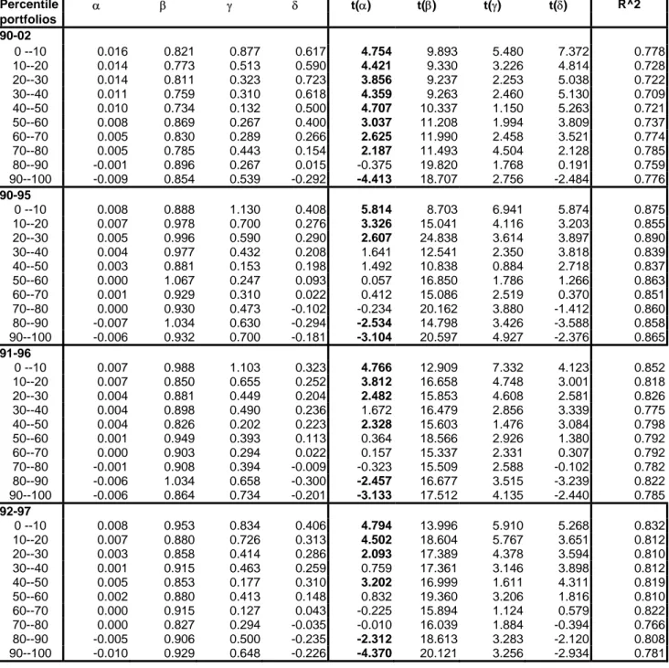
Fama-French (1995) demonstrate that intercept coefficients of 3-CAPM regressions are not significantly different from zero and argue that this proofs that returns premia on their factor portfolios are explained by latent risk factors captured by the two additional regressors and not by a failure of market efficiency. To check whether excess returns from our short term value strategies persist after being risk-adjusted, we follow Clare et. al. (1997) and Bagella et al. (2001) in estimating a system of time-series CAPM equations of monthly portfolio excess returns on those of an equally weighted market index, to explain returns from each set of the ten considered portfolios.

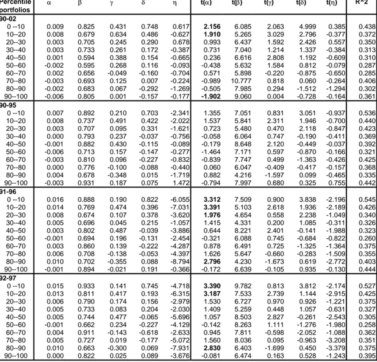
two additional risk factors, related to size and book to market values, are added to the traditional specification15_{. After it, since the excess returns are still} significantly positive, by combining Fama and French (1995) and Harvey and Siddique (2000) approaches, we extend the 3-factor CAPM to a 4-factor CAPM model, in which an additional risk factor, related to return’s skewness, is added (Harvey-Siddique 2000).

The rationale for the introduction of this fourth factor is that it is intuitively clear that the (nonnormal) unconditional return distributions cannot be adequately characterized by mean and variance alone since, coeteris paribus, right-skewed porftolios are preferred to mean-variance equivalent left-skewed portfolios. As a consequence, the latter should have lower expected returns.

Therefore, if asset returns have systematic skewness, expected returns should include rewards for accepting this risk. We formalize this intuition with a non linear specification which includes in the 3-factor CAPM equation an additional regressor which tries to capture the effect of skewness on observed returns (Tables 5C and 5D). Our choice is also consistent with Ghysels’ findings (1998) showing that nonlinear multifactor models are empirically more successful than linear beta models. Our 4-factor equation is written as follows:

t P f t m t P t P t P f t m t P P f t P t R R HML SMB R R R R − =α +β ( − )+γ +δ +η ( − )2 +ε (3)

15 _{The rationale for adopting a multifactor capital asset pricing model is that some risk factors, to} which small firms or financially distressed firms are particularly exposed, are not captured by portfolio’s sensitivity to the stock market index. Shocks in asset values may for instance reduce the value of collateral affecting both solvency of financially distressed firms and the capacity to obtain credit of small firms in a framework of imperfect information (Bernanke and Gertler, 1987). Debt deflation may negatively affect financially distressed (low MTBV) firms more than others. Expectations of liquidity squeezes, in economies in which the three Kashyap, Lamont and Stein (1993) conditions for the existence of a “credit channel” may be applied, may generate negative

where Rp is the monthly return of portfolio p (p=1,..,10), Rf is the monthly return of the 3-month treasury bill rate, Rm is the monthly return of the market portfolio, while SMB, HML and 2

)

(Rtm −Rtf are three additional risk factors16. In

order to test the stability of contrarian strategy premia, we estimate the system recursively from 1990 to 2002 using a five year window.

We estimate the system by using the GMM-HAC (Generalised Method of Moments Heteroskedasticity and Autocorrelation Consistent)17 _{approach which} sets the calculated correlations of the instruments and disturbances as close as possible to zero, according to a criterion provided by a weighting matrix (for a similar approach see MacKinlay and Richardson 1991; Bagella, Becchetti and Carpentieri 2000 and Clare et. al. 1997). GMM regressions rely on weaker assumptions than OLS as it does not require normality and constancy of variance. These two conditions are generally not met by short horizon stock returns which are usually characterised by excess curtosis and volatility clustering (Campbell, Lo and MacKinlay, 1997). As in Clare et. al. (1997), the same regressors are used as instruments (tables 5A-5D).

The estimates also show that value portfolios for the EU sample tend to be more exposed (with a more stable relationship) to book to market risk factors than size factors, while for the US sample this is true only for the period from 1994 to 2002. The interesting finding is that, differently from what occurs when looking at (small vs large) size and (low vs high) book to market portfolios

16 _{The first two additional risk factors are computed as follows. We first divide the two samples} each month into two subgroups: the 50% largest firms (group B) and the 50% smallest firms (group S). These two subgroups are then divided in turn into three subgroups containing respectively the largest 30% (group BH and SH), the mid 40% (group BM and SM) and the

French, 1998) value strategies’ exposure to the two FF additional risk factors is very similar to that of growth strategies.

Our results also show that the effect of skewness helps to explain the cross-sectional variation of expected returns across assets and is significant even when factors based on size and book-to-market are included.

Value strategies still yield significant excess returns after being adjusted for the four risk factors.

The intercept for the 0-10 value portfolios drops from 1 basis points per month for the EU and 1.6 basis points per month for the US (for the all sample period) in the 3-factor to 0.9 basis points per month for the EU and 1.2 basis points per month for the US in the 4-factor. Similarly, the intercept for the 90-100 growth portfolios for the US rises from –0.9 basis points per month in the 3-factor to –0.7 basis points per month in the 4-3-factor, while for the EU it remains stable to–0.6 basis points per month.

The model for the US sample does capture more of the variation in average returns on the portfolio than the model for the EU sample. Indeed, the average of the 10-regression R2 _{for the all period is only about 0.35 for the EU sample and} 0.7 for the US sample.

To avoid the risk that covariances across the ten portfolios residuals bias our results we re-estimate the model as a ten-equation system. We construct a Wald test of the joint hypothesis that αp =0 for all portfolios (whether all intercepts are zero). The Wald test, which is a test of mean variance efficiency, is distributed as a χ2_{(10) under the null hypothesis, where 10 is the number of} restrictions. We also test the restriction: α1=α10 (distributed as a χ2) to check the

hypothesis that the 0-10 (extreme value) portfolio has excess returns which significantly outperform those of the 90-100 (extreme growth) portfolio.

Our evidence indicates that positive excess returns of the extreme 1-month value (0-10) portfolio for the overall sample period (1990-2002) persist after risk adjustment (and the null hypothesis of Wald tests are rejected) for both EU and US sample and for both 3 and 4-factor CAPM model (Tables 6A-6D).. The analysis of the subperiods shows that the value portfolio excess returns are significantly higher than the risk-free rate for all the rolling subperiods for both samples,. with the exception of the EU sample at the beginning of our sample period (the first five years window: 1990-1995) with the 3-CAPM model and of the beginning and of the end (respectively 1990-1995 and 1997-2002) with the 4-CAPM model, when the α-coefficient is not significant. Wald test results show that the joint hypothesis that αp =0 for p =1. …, 10 and α1=α10 (Tables 6A-6D) are rejected in all subperiods. These results imply the rejection of the mean variance efficiency hypothesis and confirm that value portfolios outperform growth portfolios.

6. Conclusions

A significant share of financial investors bases their trading decisions on the evaluation of the DCF (discounted cash flow) fundamental value of a stock regarded as the gravity centre around which prices move in the medium/long run. This paper aims at testing the relative profitability of fundamentalist trading strategies on the S&P500 and on the DJSTOXX constituents in the last decades.

In doing so the paper considers a simple DCF fundamental in which I/B/E/S earning forecasts are the only reference for dertermining the gravity centre of the stock value.

Results on the relative performance of DCF value and growth strategies in the last twelve years seem to support the hypothesis that value portfolios yield significant excess returns after risk adjustment.

One month value strategies (based on a monthly selection of the stocks with the lowest observed to fundamental ratio in the previous period) yield significantly higher mean monthly returns than both corresponding growth and buy and hold strategies for both US and EU market. These results persist when returns are adjusted for risk, since risk adjusted intercepts of excess returns of value portfolios in four factor CAPM estimates are still positive and significant. The success of contrarian strategies seem not to be country specific and therefore not depending on specific features of different financial systems.

References

Adriani F. Becchetti L., 2003, Do Hig-tech stock prices revert to their fundamental value?, Applied Financial Economics, forth.

Bagella, M. Becchetti, L. Carpentieri, A., 2000, “The First Shall Be Last”. Size and value strategy premia at the London Stock Exchange, Journal of Banking and

Finance, 24(6) , pp. 893-920.

Ball, R. and Kothari, S. P., 1998, Nonstationary Expected Returns: Implications for Tests of Market Efficiency and Serial Correlation in Returns; Journal of

Financial Economics, 25, (1), pp. 51-74

Basu, S., 1983. The relationship between earning yield, market value, and return for NYSE common stocks. Journal of Financial Economics, 12, pp. 126--156

Becchetti, L., Marini G., 2003, Can we beat the Dow ? The mirage of growth strategies, CEIS Working Paper, n. 156 and Research in Research in banking and

Finance, 3, pp. 187-221.

Becchetti, L. Trovato, G., 2002, The determinants of growth of small and medium sized firms. The role of the availability of external finance, Small Business

Economics, 19, pp. 291-306

Becchetti, L. Cavallo, L., 2001, Shrinking size premia at the LSE, Research in

banking and Finance, 2, pp. 265-298 .

Bernanke, B.S. and M. Gertler, 1987, Financial Fragility and Economic Performance, NBER, Working Paper 2318.

Black. F., 1993. Beta and Return. Journal of Portfolio Management 20, pp. 8--18.

Breeden, D.T., Gibbons, M.R., Litzemberger, R.H., 1989. Empirical tests of the consumption-oriented CAPM. Journal of Finance 44 (2), pp. 231--62.

Campbell, J.Y., Lo, A.W. and Mackinlay, A.C., 1997, The Econometrics of Financial Markets, Princeton University Press.

Capual C., Ian Rowley and W. F. Sharpe, 1993, International value and growth stock returns, Financial Analysts Journal, January-February, 27-36.

Chan K.C. “On the contrarian investment strategy” 1988.

Chan, K.C., Hamao Y., Lakonishok, J., 1991. Fundamentals and stock returns in Japan. Journal of Finance 46, pp. 1739--1789

Clare, Smith and Thomas, 1997, UK stock returns and robust tests of mean-variance efficiency, Journal of Banking and Finance, pp. 641-660.

Corrado C. and Zivney C., 1992, The specification and power of sign test in event study hypothesis tests using stock returns, Journal of Financial and Quantitative Analysis, 27, 465-78.

De Bondt W.-Thaler R., 1985, Does the stock market overreact?, Journal of

Finance, 40, 793-808.

De Long, J.B., A. Shleifer, L. Summers and R.J. Waldmann, 1990, 'Noise Trader Risk in Financial Markets', Journal of Political Economy, vol. 98, pp.701-738. Devereaux, M. and F. Schiantarelli, 1989,Investment, Financial Factors, and Cash Flow: evidence from UK Panel Data, NBER Working Paper 3116.

Fama, E.F. and K.R. French, 1992, The Cross-section of expected stock returns,

Fama, E.F., French, K.R., 1995. Size and book-to-market factors in earnings and returns. Journal of Finance, 50. pp. 131--156.

Fama, E.F. and K.R. French, 1996, Multifactor explanations of asset pricing anomalies, Journal of Finance, 51 (1), pp. 55-84.

Fama, E.F. and K.R. French, 1998, Value versus growth: the international evidence, Journal of Finance, 53, ( 6), pp. 1975-99

Foster F. D., T. Smith and R. E. Whaley, 1997, Assessing goodness-of-fit of asset pricing modes: The distribution of the maximal R2 _{Journal of Finance, 52, pp.} 597-607.

Frankel, J.A., Froot, K.A., 1990, Chartists, fundamentalists, and trading in the foreign exchange market, American Economic Review (paper and proceedings) 80,

181-85.

Frankel, R. and Lee, C. M. C., June 1998, Accounting Valuation, Market Expectation, and Cross-Sectional Stock Returns, Journal of Accounting and

Economics; 25(3), pp. 283-319.

Ghysels E., 1998, On stable factor strucutres in the pricing of risk: Do time-varying betas help or hurt?, Journal of Finance, 53, 457-482.

Gordon M. and Shapiro E. (1956) "Capital Equipment Analysis, the Required Rate of Profit" Management Science, pp.102-110.

Hansen, L., 1982. Large sample properties of generalised methods of moments estimators. Econometrica 50, pp. 1029--1054.

Hansen, L., Singleton, K., 1982. Generalised instrumental variables estimation in non-linear rational expectations models. Econometrica 50, pp. 1269--1286.

Harvey, C. R. and Siddique, A., 2000, Conditional Skewness in Asset Pricing Tests; Journal of Finance, 55, (3), pp. 1263-95

Haugen R., 1995, The New Finance: The Case against Efficient Markets (Prentice Hall, Englewood Cliffs, N. J.)

Jagannathan, R. and Wang Z., 1996 , The conditional CAPM and the cross-section of expected returns, The Journal of Finance 51(1), pp.3-53.

Jeegadesh, N. Titman S., 1993, Returns to buying winners and selling losers: implications for stock market efficiency, Journal of Finance, 48 (1), pp. 65-91. Kaplan S.N., Roeback, R.S., 1995, The valuation of cash flow forecasts: an empirical analysis, Journal of Finance, 50 (4), pp. 1059-1093.

Kashyap A.K., Lamont, O., Stein, J.C., 1993. Credit conditions and the cyclical behaviour of inventories. Federal Reserve Bank of Chicago, Working Paper n. 7. Kothari S.P., Jay Shanken and R. G. Sloan, 1995, Another look at the cross-section of expected stock returns, Journal of Finance, 50, 185-224.

Li, H. and Xu, Y., 2002, Survival Bias and the Equity Premium Puzzle, Journal of Finance

Lakonishok, J., Shleifer, A. and R.W. Vishny, 1994, Contrarian investment, extrapolation and risk, Journal of Finance, 49, pp. 1541-1578.

Lee, C. M. C.; Myers J. and Swaminathan, B., 1999, What Is the Intrinsic Value of the Dow?, Journal of Finance; 54(5), pp. 1693-1741.

Linter, J., 1965. The valuation of risk assets and the selection of risky investments in stock portfolios and capital budgets. Review of Economics and Statistics 47, pp. 13--37.

Lo, A., MacKinlay, 1990, When are contrarian profits due to stock market overreaction ?, Review of Financial Studies, 3 (2), pp.175-208.

MacKinlay A. and Richardson M., 1991, Using generalised method of moments to test mean-variance efficiency, Journal of Finance 46 (2), 511-527.

Miller M. H. and Modigliani F., 1961, Dividend Policy, Growth and the Valuation of Shares Journal of Business, pp.411-33.

Pagan A. and Schwert W., 1990, Alternative methods for conditional stock volatility, Journal of Econometrics, 45, 267-90.

Rosenberg, B., Reid, K., Lanstein, R., 1985. Persuasive evidence of market inefficiency. Journal of Portfolio Management, 11, pp. 9--17.

Rouwenhorst, K.G., 1998, International momentum strategies, Journal of

Finance, 53, pp.267-285

Sethi, R., 1996, Endogenous Regime Switching in Speculative Markets, Structural Change and Economic Dynamics; 7(1), pp. 99-118.

Sharpe, W.F., 1964. Capital asset prices: a theory of market equilibrium under conditions of risk, Journal of Finance 19, pp. 425--442.

Shumway, T., 1997. The Delisting bias in CRSP data. Journal of Finance 52, pp. 327-340.

Wang, Y., 1993, Near Rational Behaviour and Financial Market Fluctuations, The Economic Journal, 103, 1462-1478.

Zivney T. and Thompson D., 1989, The specification and power of the sign test in measuring security price performance: comments and analysis, Financial Review, 24, 581-8.

Appendix

Legend for tables 1.A-1.F:

SUMMARY STATISTICS for AVERAGE MONTHLY PERCENT RETURNS on equal-weight deciles formed on observed to fundamental ratio: 01/1990-03/2002, 147 months.

The 10 Portfolios (from 0-10 to 90-100) are formed according to ascending values of the observed to fundamental ratio (i.e. the first portfolio includes stocks whose observed to fundamental ratio falls in the lowest ten percent of the distribution in the considered month). Portfolios are formed the first day of month t on values that the ranking variable assumes in the last day of the month t-1 and held until the end of the month t (1 month strategy), t+1 (2 months strategy), t+6 (6 months strategy), t+12 (12 months strategy). New portfolios are formed only at the end of each holding period.

The benchmark is the passive buy and hold strategy on the total sample portfolio and on the stock market index (S&P500 for the US and DJSTOXX for the EU).

The sharpe ratio is calculated as: [Rp-Rf]/σp where Rp is the mean monthly return of the p-th portfolio

(p=1,…,10), Rf is the monthly risk-free rate, and σp is the standard deviation of the Rp.

Table 1.A EU: MEAN, VARIANCE and SKEWNESS of MONTHLY RETURNS from VALUE and GROWTH DCF strategies on DJSTOXX

(risk premium 7%; nominal rate of growth in the terminal period 3%)

1990-2002

0-10 10-20 20-30 30-40 40-50 50-60 60-70 70-80 80-90 90-100 buy-hold MEAN monthly returns (percent values)

1month 1.309 1.209 0.965 0.827 0.581 0.422 0.815 0.370 0.453 0.129 0.708 2 months 1.264 1.021 1.095 0.976 0.581 0.488 0.587 0.590 0.545 0.010 TSP* 6 months 1.360 1.031 1.126 0.780 0.743 0.564 0.379 0.451 0.467 0.313 0.702 12months 1.384 1.151 1.096 0.814 0.746 0.352 0.690 0.349 0.186 0.458 DJSTOX VARIANCE 1month 0.004 0.004 0.003 0.003 0.003 0.002 0.002 0.002 0.003 0.003 2 months 0.002 0.001 0.001 0.001 0.001 0.001 0.001 0.001 0.001 0.001 0.002 6 months 0.001 0.001 0.001 0.001 0.000 0.000 0.000 0.000 0.000 0.000 12months 0.000 0.000 0.000 0.000 0.000 0.000 0.000 0.000 0.000 0.000 SKEWNESS 1month -0.641 -1.185 -0.295 -1.234 -0.496 -0.342 0.148 -0.510 -0.483 -0.468 2 months -0.563 -0.556 -0.519 -0.205 -0.640 -0.425 -0.166 -0.244 0.031 -0.258 -0.843 6 months 0.265 -0.093 0.014 -0.386 0.041 -0.061 -0.449 0.144 -0.139 -0.213 12months -0.429 -0.201 -0.684 -0.544 -0.013 -1.316 -0.018 -1.099 -0.107 -0.058 SHARPE RATIO 1month 0.131 0.118 0.092 0.059 0.017 -0.015 0.065 -0.028 -0.008 -0.068 2 months 0.177 0.140 0.161 0.131 0.028 -0.001 0.025 0.032 0.015 -0.133 6 months 0.329 0.224 0.259 0.117 0.115 0.036 -0.056 -0.030 -0.016 -0.098 12months 0.430 0.457 0.338 0.160 0.160 -0.101 0.149 -0.141 -0.199 -0.026 MV/1000 37537.5 56695.9 93140.6 138259.3 230386.0 350929.2 369168.3 791921.7 1289230.2 794773.0 TSP* = Total sample portfolio.

Table 1.B US: MEAN, VARIANCE and SKEWNESS of MONTHLY RETURNS from VALUE and GROWTH DCF strategies on S&P500

(risk premium 7%; nominal rate of growth in the terminal period 3%)

1990-2002

0-10 10-20 20-30 30-40 40-50 50-60 60-70 70-80 80-90 90-100 buy-hold

MEAN monthly returns (percent values)

1month 1.017 0.947 0.697 0.656 0.735 0.748 0.709 0.827 0.597 0.287 0.722 2 months 0.916 0.874 0.630 0.760 0.698 0.743 0.725 0.844 0.626 0.440 TSP* 6 months 0.908 0.651 0.702 0.651 0.586 0.882 0.739 0.769 0.623 0.664 0.797 12months 0.904 0.684 0.644 0.757 0.753 0.739 0.753 0.909 0.486 0.539 S&P500 VARIANCE 1month 0.003 0.002 0.002 0.002 0.001 0.002 0.002 0.002 0.002 0.002 2 months 0.002 0.001 0.001 0.001 0.001 0.001 0.001 0.001 0.001 0.001 6 months 0.000 0.000 0.000 0.000 0.000 0.000 0.000 0.000 0.000 0.000 0.002 12 months 0.000 0.000 0.000 0.000 0.000 0.000 0.000 0.000 0.000 0.000 SKEWNESS 1month -0.290 -0.162 -0.020 -0.493 -0.516 -0.132 -0.369 -0.071 -0.293 -0.664 2 months -0.876 -0.554 -0.414 -0.487 -1.046 -0.624 -0.664 -0.331 -0.846 -0.417 -0.268 6 months -0.214 -0.946 -1.186 -0.557 -0.710 -0.641 -0.323 -0.140 -0.678 -0.786 12 months -0.250 -0.306 -0.825 -0.147 -0.132 -0.194 0.233 0.035 -0.568 -0.921 SHARPE RATIO 1month -0.742 -0.850 -0.881 -0.960 -1.071 -0.925 -1.016 -1.015 -0.988 -1.043 2 months 0.130 0.135 0.066 0.112 0.097 0.118 0.119 0.151 0.074 0.016 6 months 0.253 0.135 0.164 0.147 0.109 0.344 0.284 0.234 0.146 0.161 12 months 0.355 0.187 0.177 0.264 0.303 0.305 0.379 0.444 0.059 0.087

Table 1.C EU: MEAN, VARIANCE and SKEWNESS of MONTHLY RETURNS from VALUE and GROWTH DCF strategies on DJSTOXX

(risk premium 7%; nominal rate of growth in the terminal period 3%)

1990-1995

0-10 10-20 20-30 30-40 40-50 50-60 60-70 70-80 80-90 90-100 buy-hold

MEAN monthly returns (percent values)

1month 0.480 0.837 0.412 0.356 0.399 -0.099 0.178 0.446 0.650 0.211 0.388 2 months 0.540 0.748 0.446 0.409 0.345 -0.096 0.020 0.447 0.771 0.011 TSP* 6 months 0.646 0.572 0.418 0.275 0.240 0.023 0.050 0.535 0.539 0.266 0.367 12months 0.405 0.831 0.303 0.325 0.349 -0.118 0.145 0.226 0.471 0.342 DJSTOX VARIANCE 1month 0.003 0.002 0.002 0.002 0.002 0.002 0.002 0.002 0.002 0.002 2 months 0.002 0.001 0.001 0.001 0.001 0.001 0.001 0.001 0.001 0.001 0.002 6 months 0.001 0.001 0.001 0.001 0.000 0.000 0.000 0.000 0.000 0.000 12months 0.001 0.000 0.000 0.000 0.000 0.000 0.000 0.000 0.000 0.000 SKEWNESS 1month -0.487 -0.125 -0.133 -0.821 -0.462 -0.212 -0.612 -0.392 -0.564 -0.420 2 months -0.378 -0.266 -0.567 -0.707 -0.307 -0.147 -0.728 -0.167 -0.639 -0.204 0.002 6 months -0.015 -0.201 -0.190 -0.782 -0.791 0.016 -0.581 -0.576 -0.466 -0.353 12months 0.778 0.520 -0.617 0.023 0.164 -1.702 1.092 -0.245 0.545 0.449 SHARPE RATIO 1month -0.033 0.039 -0.057 -0.065 -0.052 -0.176 -0.112 -0.048 -0.001 -0.094 2 months -0.028 0.027 -0.059 -0.077 -0.090 -0.236 -0.193 -0.070 0.033 -0.179 6 months -0.010 -0.043 -0.109 -0.165 -0.196 -0.336 -0.289 -0.118 -0.091 -0.191 12months -0.113 0.078 -0.195 -0.182 -0.249 -0.472 -0.537 -0.453 -0.149 -0.248 TSP* = Total sample portfolio.

Table 1.D US: MEAN, VARIANCE and SKEWNESS of MONTHLY RETURNS from VALUE and GROWTH DCF strategies on S&P500

(risk premium 7%; nominal rate of growth in the terminal period 3%)

1990-1995

0-10 10-20 20-30 30-40 40-50 50-60 60-70 70-80 80-90 90-100 buy-hold MEAN monthly returns (percent values)

1month 1.121 1.153 0.880 0.888 0.737 0.701 0.826 0.931 0.612 0.504 0.835 2 months 1.040 0.976 0.805 0.854 0.737 0.787 0.588 0.923 0.630 0.559 TSP* 6 months 0.983 0.800 1.010 0.826 0.551 0.613 0.765 0.837 0.746 0.705 0.762 12months 0.702 0.373 0.561 0.583 0.423 0.445 0.879 0.897 0.566 0.478 S&P500 VARIANCE 1month 0.002 0.002 0.002 0.001 0.001 0.001 0.001 0.001 0.002 0.001 2 months 0.001 0.001 0.001 0.001 0.001 0.001 0.001 0.001 0.001 0.001 0.001 6 months 0.000 0.000 0.000 0.000 0.000 0.000 0.000 0.000 0.000 0.000 12months 0.000 0.000 0.000 0.000 0.000 0.000 0.000 0.000 0.000 0.000 SKEWNESS 1month -0.295 -0.517 -0.260 -0.722 -1.291 -0.450 -0.336 0.266 -0.231 -0.081 2 months 0.043 -0.650 -0.787 -0.109 -1.289 -1.222 -0.333 0.142 -0.489 -0.127 -0.369 6 months 0.064 0.151 -0.934 0.632 -0.273 -0.649 -0.838 0.972 -0.001 0.230 12months -0.006 0.212 -0.112 1.088 0.211 0.437 -0.124 1.184 0.715 0.778 SHARPE RATIO 1month -0.867 -0.927 -1.027 -1.072 -1.328 -1.125 -1.219 -1.148 -1.094 -1.199 2 months 0.180 0.174 0.128 0.160 0.144 0.156 0.078 0.198 0.081 0.057 6 months 0.271 0.244 0.355 0.286 0.098 0.139 0.281 0.329 0.234 0.217 12months 0.185 -0.011 0.122 0.167 0.029 0.059 0.532 0.450 0.132 0.059

Table 1.E EU: MEAN, VARIANCE and SKEWNESS of MONTHLY RETURNS from VALUE and GROWTH DCF strategies on DJSTOXX

(risk premium 7%; nominal rate of growth in the terminal period 3%)

1996-2002

0-10 10-20 20-30 30-40 40-50 50-60 60-70 70-80 80-90 90-100 buy-hold MEAN monthly returns (percent values)

1month 2.094 1.560 1.488 1.272 0.753 0.915 1.418 0.299 0.266 0.051 1.01 2 months 1.930 1.273 1.693 1.498 0.799 1.026 1.110 0.721 0.338 0.010 TSP* 6 months 1.964 1.419 1.724 1.207 1.169 1.021 0.658 0.379 0.407 0.352 0.990 12months 2.084 1.380 1.663 1.163 1.028 0.688 1.080 0.438 -0.018 0.541 DJSTOX VARIAN CE 1month 0.003 0.002 0.002 0.002 0.002 0.002 0.002 0.002 0.002 0.002 2 months 0.002 0.002 0.001 0.002 0.001 0.001 0.002 0.001 0.001 0.001 0.003 6 months 0.001 0.001 0.001 0.001 0.000 0.000 0.000 0.000 0.000 0.000 12 months 0.000 0.000 0.000 0.000 0.000 0.000 0.000 0.000 0.000 0.000 SKEWN ESS 1month -0.653 -0.315 -0.264 -0.965 -0.662 -0.323 0.728 -0.703 -0.694 -0.583 2 months -0.814 -0.784 -0.582 -0.122 -1.107 -0.735 -0.020 -0.327 0.639 -0.317 0.002 6 months 0.481 -0.064 0.152 -0.115 1.097 0.093 -0.301 0.409 0.006 0.054 12 months -0.885 -0.987 0.196 -1.134 -0.272 0.225 -0.777 -1.981 -0.397 -0.375 SHARPE RATIO 1month 0.338 0.261 0.268 0.209 0.088 0.138 0.216 -0.011 -0.018 -0.066 2 months 0.362 0.229 0.358 0.288 0.161 0.217 0.191 0.123 -0.001 -0.091 6 months 0.622 0.450 0.582 0.364 0.408 0.396 0.159 0.018 0.029 0.002 12 months 1.347 0.994 0.966 0.428 0.414 0.310 0.538 0.077 -0.236 0.127

TSP* = Total sample portfolio.

Table 1.F US: MEAN, VARIANCE and SKEWNESS of MONTHLY RETURNS from VALUE and GROWTH DCF strategies on S&P500

(risk premium 7%; nominal rate of growth in the terminal period 3%)

1996-2002

0-10 ott-20 20-30 30-40 40-50 50-60 60-70 70-80 80-90 90-100 buy-hold MEAN monthly returns (percent values)

1month 0.918 0.751 0.523 0.437 0.734 0.792 0.598 0.728 0.583 0.082 0.616 2 months 0.802 0.781 0.469 0.674 0.663 0.701 0.851 0.770 0.621 0.329 6 months 0.848 0.535 0.460 0.513 0.614 1.093 0.719 0.716 0.527 0.633 0.831 12months 1.048 0.906 0.703 0.881 0.989 0.949 0.663 0.918 0.428 0.584 S&P500 VARIANCE 1month 0.003 0.003 0.003 0.002 0.002 0.003 0.002 0.002 0.002 0.002 2 months 0.002 0.001 0.002 0.001 0.001 0.001 0.001 0.001 0.001 0.001 0.002 6 months 0.000 0.000 0.000 0.000 0.000 0.000 0.000 0.000 0.000 0.000 12months 0.000 0.000 0.000 0.000 0.000 0.000 0.000 0.000 0.000 0.000 SKEWNESS 1month -0.259 0.057 0.117 -0.331 -0.225 -0.013 -0.333 -0.206 -0.327 -0.825 2 months -1.306 -0.491 -0.191 -0.629 -0.916 -0.367 -0.864 -0.549 -1.064 -0.716 6 months -0.668 -1.509 -1.542 -1.060 -1.036 -0.432 0.311 -0.520 -1.279 -1.230 -0.190 12months -0.342 -0.733 -1.547 -0.672 -0.494 -0.708 0.535 -0.601 -1.166 -1.814 SHARPE RATIO 1month -0.665 -0.800 -0.797 -0.893 -0.920 -0.798 -0.899 -0.927 -0.907 -0.952 2 months 0.094 0.104 0.020 0.079 0.074 0.094 0.151 0.117 0.069 -0.023 6 months 0.249 0.069 0.032 0.062 0.121 0.582 0.301 0.186 0.083 0.132 12months 0.393 0.245 0.087 0.203 0.342 0.305 0.085 0.288 -0.102 0.000

Table 2.A EU: Significance of the difference in unconditional mean monthly returns of different portfolio strategies

Holding period Significance of differ. in MMRs

Compared strategies T TEST Non param.

test

Z prob>Z

1month 2.9016 1.933 0.0532

2months VALUE vs 3.1362 2.123 0.0337

6months GROWTH porfolio 2.8655 1.382 0.1671

12months 2.3296 1.386 0.1659

1month buyhold vs GROWTH -2.247 -1.035 0.3008

buyhold vs VALUE 2.5389 1.121 0.2624

2months buyhold vs GROWTH -2.7362 -1.227 0.2198

buyhold vs VALUE 2.403 1.121 0.2621

6months buyhold vs GROWTH -2.2181 -0.742 0.4579

buyhold vs VALUE 2.3948 0.784 0.4333

12months buyhold vs GROWTH -1.3354 -0.52 0.6033

buyhold vs VALUE 2.2724 0.924 0.3556

Table 2.B US: Significance of the difference in unconditional mean monthly returns of different portfolio strategies

Holding period Significance of differ. in MMRs

of strategies Compared strategies T TEST Non param.

test

Z prob>Z

1month 2.116 1.250 0.2112

2months GROWTH vs 1.209 1.47 0.1417

6months VALUE porfolio 0.514 0.577 0.5637

12months 0.762 0.231 0.8174

1month buyhold vs GROWTH -1.8712 -0.545 0.5859

buyhold vs VALUE 1.4454 0.796 0.4292

2months buyhold vs GROWTH -1.1125 -0.836 0.4034

buyhold vs VALUE 0.9195 0.761 0.4465

6months buyhold vs GROWTH -0.1774 0.082 0.9343

buyhold vs VALUE 0.8086 0.619 0.5362

12months buyhold vs GROWTH -0.5692 -0.058 0.9540

buyhold vs VALUE 0.7651 0.577 0.5637

The non parametric test is based on the Mann-Withney U-statistics computed as follows:U = N N_{1 2} + N N1 1+1 −R₁ 2 ( ) and U =N N_{1 2} + N2 N2+1 −R₂ 2 ( )

where N₁ is the number of observations in the first sample, N₂ is the number of observations in the second sample, R₁ is the sum of ranks in the first sample, R₂ is the sum of ranks in the second sample. The test is based on the lowest of the U values.

Table 3.A EU: Covariance between portfolio quarterly returns and GDP rate of growth Percentile 90-02 90-95 96-02 portfolios 0 --10 -1.454 -0.929 -3.028 10--20 -2.430 -0.534 -2.949 20--30 -0.994 -0.619 -1.551 30--40 -2.679 -0.758 -1.702 40--50 -2.437 -0.364 -2.137 50--60 -1.725 -0.857 -1.959 60--70 -0.029 0.117 -2.069 70--80 -3.882 -0.138 -1.688 80--90 -0.428 -0.419 -1.569 90--100 -1.431 -0.829 -0.194

Table 3.B US: Covariance between portfolio quarterly returns and GDP rate of growth Percentile 90-02 90-95 96-02 portfolios 0 --10 -24.419 2.294 -17.881 10--20 -4.880 3.353 -3.758 20--30 -7.771 2.009 -3.777 30--40 -1.719 4.368 -6.838 40--50 -0.328 2.990 -3.916 50--60 -1.604 -0.521 -0.579 60--70 -3.408 2.874 -2.310 70--80 -4.962 1.068 -3.077 80--90 -11.881 1.268 -10.011 90--100 -8.681 2.583 -11.692

Table 4 Correlation of US and European value portfolios

Percentile 90-02 90-95 96-02 portfolios 0 --10 0.00201 0.00129 0.00271 10--20 0.00154 0.00091 0.00215 20--30 0.00133 0.00095 0.00171 30--40 0.00138 0.00087 0.00189 40--50 0.00111 0.00090 0.00130 50--60 0.00139 0.00090 0.00185 60--70 0.00127 0.00075 0.00178 70--80 0.00104 0.00086 0.00121 80--90 0.00110 0.00074 0.00144 90--100 0.00141 0.00078 0.00200

Legend for tables 5.A-5.D

THREE and FOUR-FACTOR TIME-SERIES REGRESSIONS for Monthly Excess Returns on equal-weight deciles: 01/1990-03/2002, 147 months.

The table reports coefficients and t-tests of a 3-CAPM system composed by p equations. The p-th equation is written as follows: t P f t m t P t P t P f t m t P P f t P t R R HML SMB R R R R − =α +β ( − )+γ +δ +η ( − )2 +ε

where Rp is the monthly return of portfolio p (p=1,..,10), Rf is the monthly return of the 1-month Treasury

bill rate, Rm is the monthly return of the market portfolio while SMB and HML are additional risk factors.

The 10 Portfolios (from 0-10 to 90-100) are formed according to ascending values of the observed to fundamental ratio (i.e. the first portfolio includes stocks whose observed to fundamental ratio falls in the lowest ten percent of the distribution in the considered month). Portfolios are formed the first day of month t on values that the ranking variable assumes in the last day of the month t-1 and held until the end of the month t (1 month strategy). New portfolios are formed only at the end of each holding period.

The system is estimated recursively from 1990 to 2002 using a five year window with a GMM (Generalised Method of Moments) approach with Heteroskedasticity and Autocorrelation Consistent Covariance Matrix. The Bartlett’s functional form of the kernel is used to weight the covariances in calculating the weighting matrix. Newey and West’s (1994) automatic bandwidth procedure is adopted to determine weights inside kernels for autocovariances.

The same regressors are used as instruments.

Table 5.A EU: RISK ADJUSTMENT OF RETURNS with 3-CAPM model (10 equations system estimated by GMM simultaneusly) DJSTOXX

(risk premium 7%; nominal rate of growth in the terminal period 3%) Percentile α β γ δ t(α) t(β) t(γ) t(δ) R^2 portfolios 90-02 0 --10 0.010 0.813 0.436 0.740 2.976 5.902 2.073 4.964 0.437 10--20 0.007 0.691 0.629 0.495 2.396 5.264 2.905 2.735 0.372 20--30 0.004 0.691 0.251 0.280 1.509 6.985 1.633 2.342 0.349 30--40 0.002 0.740 0.258 0.177 0.668 7.033 1.184 1.350 0.312 40--50 0.000 0.608 0.382 0.163 -0.099 6.536 2.670 1.267 0.309 50--60 -0.002 0.597 0.267 0.118 -0.581 5.893 1.558 0.817 0.287 60--70 0.001 0.670 -0.055 -0.150 0.324 5.946 -0.243 -0.822 0.283 70--80 -0.003 0.697 0.123 0.010 -1.378 10.298 0.796 0.086 0.406 80--90 -0.004 0.708 0.056 -0.274 -1.142 8.759 0.242 -1.376 0.298 90--100 -0.006 0.808 -0.001 -0.154 -2.049 9.398 -0.005 -0.717 0.361 90-95 0 --10 0.005 0.947 0.208 0.700 1.099 6.851 0.786 2.950 0.528 10--20 0.006 0.785 0.490 0.419 1.740 6.065 2.202 1.890 0.433 20--30 0.001 0.745 0.094 0.329 0.413 6.189 0.447 2.075 0.417 30--40 -0.001 0.811 0.237 -0.038 -0.291 6.298 0.739 -0.195 0.368 40--50 -0.001 0.884 0.430 -0.115 -0.256 8.647 2.113 -0.450 0.392 50--60 -0.006 0.719 0.157 -0.148 -1.876 8.177 0.593 -0.871 0.320 60--70 -0.004 0.830 0.096 -0.228 -1.427 8.190 0.487 -1.364 0.424 70--80 0.000 0.787 -0.101 -0.089 -0.069 6.925 -0.406 -0.421 0.368 80--90 0.002 0.718 -0.350 0.013 0.779 4.732 -1.549 0.084 0.330 90--100 -0.002 0.896 0.189 0.077 -0.499 8.051 0.700 0.340 0.439 91-96 0 --10 0.011 0.887 0.147 0.837 2.721 5.843 0.665 3.550 0.515 10--20 0.008 0.768 0.425 0.413 2.172 4.471 2.240 1.775 0.380 20--30 0.005 0.673 0.082 0.387 1.593 4.371 0.426 2.205 0.325 30--40 0.004 0.696 0.038 0.217 1.139 4.351 0.175 1.113 0.324 40--50 0.000 0.802 0.460 -0.029 -0.004 7.904 2.232 -0.103 0.309 50--60 -0.003 0.694 0.178 -0.125 -0.994 5.893 0.678 -0.637 0.253 60--70 -0.001 0.859 0.109 -0.212 -0.231 6.006 0.582 -1.249 0.355 70--80 0.002 0.707 -0.169 -0.042 0.795 4.964 -0.805 -0.221 0.330 80--90 0.003 0.700 -0.417 0.109 0.913 3.684 -1.980 0.722 0.321 90--100 -0.001 0.894 -0.024 0.192 -0.298 6.672 -0.120 0.937 0.444 92-97 0 --10 0.011 0.932 0.074 0.767 3.178 7.717 0.423 3.602 0.509 10--20 0.007 0.810 0.328 0.222 2.120 6.419 2.065 1.145 0.390 20--30 0.004 0.789 0.132 0.170 1.182 6.587 0.806 0.985 0.366 30--40 0.004 0.732 0.055 0.213 0.992 5.397 0.345 1.112 0.322 40--50 0.000 0.742 0.396 -0.038 0.115 6.362 2.271 -0.143 0.281 50--60 -0.004 0.661 0.176 -0.208 -1.212 6.671 0.860 -1.047 0.241 60--70 0.002 0.910 -0.180 -0.606 0.507 7.915 -0.769 -2.095 0.357 70--80 0.000 0.725 -0.053 -0.154 0.139 6.108 -0.273 -0.760 0.320 80--90 0.003 0.661 -0.413 0.105 1.095 4.762 -2.468 0.556 0.302 90--100 -0.003 0.821 -0.027 0.106 -1.154 6.319 -0.187 0.589 0.380