Geophysical time series data mining

1

U

NIVERSITÀ DEGLI

S

TUDI DI

C

ATANIA

F

S

MM.

FF.

NN.

DIPARTIMENTO DI MATEMATICA E INFORMATICA

______________________

DOTTORATO DI RICERCA IN INFORMATICA

Tesi di Dottorato

GEOPHYSICAL TIME SERIES DATA MINING

Dottorando: Tutor:

Carmelo Cassisi Alfredo Pulvirenti

Placido Montalto

3

A Maria Luisa,

e alla mia famiglia

5

Acknowledgements

It is a pleasure to thank the many people who made this thesis possible. I would like to express my deep and sincere gratitude to my supervisors, Dr. Alfredo Pulvirenti, Department of Computer Science, University of Catania, and Dr. Placido Montalto, INGV Section of Catania – Osservatorio Etneo. Their wide knowledge and their logical way of thinking have been of great value for me. Their understanding, encouraging and personal guidance have provided a good basis for the present thesis.

I warmly thank Dr. Alfredo Pulvirenti for teaching me the discipline of data mining and for introducing me to the world of research and work by accepting me as a Ph.D. student. I am grateful to other people of the Department of Computer Science, University of Catania, who supported me in research: Prof. Alfredo Ferro and Dr. Rosalba Giugno, for their encouragement and insightful comments.

My sincere thanks go to Dr. Placido Montalto for the continuous support of my Ph.D. study and research, for his patience, motivation and enthusiasm. His guidance helped me in all the time of research and writing of this thesis. Besides him, I warmly thank two special INGV colleagues, who helped me in my professional growth: Dr. Andrea Cannata and Dr. Marco Aliotta. For their kind assistance, for providing a stimulating and fun environment in which to learn and grow.

During this work I collaborated with many colleagues for whom I have great regard, and I wish to extend my warmest thanks to all those who have helped me with my work: Dr. Michele Prestifilippo, Dr. Deborah Lo Castro, Dr. Daniele Andronico and Dr. Letizia Spampinato.

The financial support of the Istituto Nazionale di Geofisica e Vulcanologia (INGV) Section of Catania – Osservatorio Etneo is gratefully acknowledged. A special thanks goes to the director Dr. Domenico Patanè for giving me the opportunity to work with an organization of such a prestige.

6

Lastly, and most importantly, I want to thank my girlfriend Maria Luisa for always believing in me and for all time spent together, advising me in every important decision, and my family, especially my parents Rosario and Donatella, which always supported me in any area of my life. I wish to thank Giuseppe and Fulvia, my friends and all relatives for all the emotional support, camaraderie, entertainment, and caring they provided. I thank also all other saints for supporting me spiritually throughout my life. In a special way my warm thanks go to Gianni and Gioacchino Paolo. All these people raised me, supported me, taught me, and loved me. To them I dedicate this thesis.

But above all, I praise God, the almighty for providing me all I need and granting me the capability to proceed successfully.

7

Preface

The process of automatic extraction, recognition, description and classification of patterns from huge amount of data plays an important role in modern volcano monitoring techniques. In particular, the ability of certain systems to recognize different volcano status can help the researchers to better understand the complex dynamics underlying the geophysical system. The geophysical data are automatically measured and recorded by geophysical instruments. Their interpretation is very important for the investigation of earth’s behavior.

The fundamental task of volcano monitoring is to follow volcanic activity and promptly recognize any changes. To achieve such goals, different geophysical techniques (i.e. seismology, ground deformation, remote sensing, magnetic and electromagnetic studies, gravimetric) are used to obtain precise measurements of the variations induced by an evolving magmatic system. To proper exploit the wealth of such heterogeneous data, algorithms and techniques of data mining are fundamental tools. This thesis can be considered a detailed report about the application of the data mining discipline in the geophysical area. After introducing the basic concepts and the most important techniques constituting the state-of-art in the data mining field, we will apply several methods able to reach important results about the extraction of unknown recurrent patterns in seismic and infrasonic signals, and we will show the implementation of systems representing efficient tools for the monitoring purpose.

The thesis is organized as follows. Chapter 1 briefly introduces to the data mining discipline; Chapter 2 discusses the similarity matching problem, explaining the importance of using efficient data structures to perform search, and the choice of adequate distance measures. It also lists the most common similarity/distance measures used for data mining, devoting a deepening part for time series similarity. Chapter 3 reviews the state-of-art dimensionality reduction techniques for the summarization of time series in data mining. Chapter 4 provides some basic principles on supervised classification, while Chapter 5 analyzes main clustering methods, for the unsupervised classification task, together with some recent developments.

8

A broad range of data mining applications will be devoted in Chapter 6, where the classification and prediction tasks are applied on geophysical data.

9

Contents

CHAPTER 1 - INTRODUCTION ... 13

1.1TYPICAL DATA MINING TASKS ... 16

1.2TIME SERIES DATA MINING ... 17

1.3DATA MINING ON GEOPHYSICS... 18

CHAPTER 2 - FUNDAMENTALS ON SIMILARITY MATCHING ... 19

2.1TYPES OF DATA ... 19

2.2INDEXING ... 20

2.3SIMILARITY AND DISTANCE MEASURES ... 22

2.3.1 Numerical Similarity Measures... 22

Mean Similarity ... 23

Root Mean Square Similarity: ... 23

Peak similarity ... 23

Cosine similarity ... 23

Cross-correlation ... 23

2.3.2 Numerical Distance Measures ... 24

Euclidean Distance ... 24

Manhattan Distance ... 24

Maximum Distance ... 24

Minkowski Distance ... 24

Mahalanobis Distance ... 25

2.3.3 Binary and Categorical Data Measures ... 25

2.3.4 Measures for Time Series Data ... 26

Dynamic Time Warping ... 28

Longest Common SubSequence ... 33

CHAPTER 3 - DIMENSIONALITY REDUCTION TECHNIQUES ... 35

3.1DFT ... 36

3.2DWT ... 39

3.3SVD ... 41

3.4DIMENSIONALITY REDUCTION VIA PAA ... 43

3.5APCA ... 44

3.6TIME SERIES SEGMENTATION USING PLA ... 46

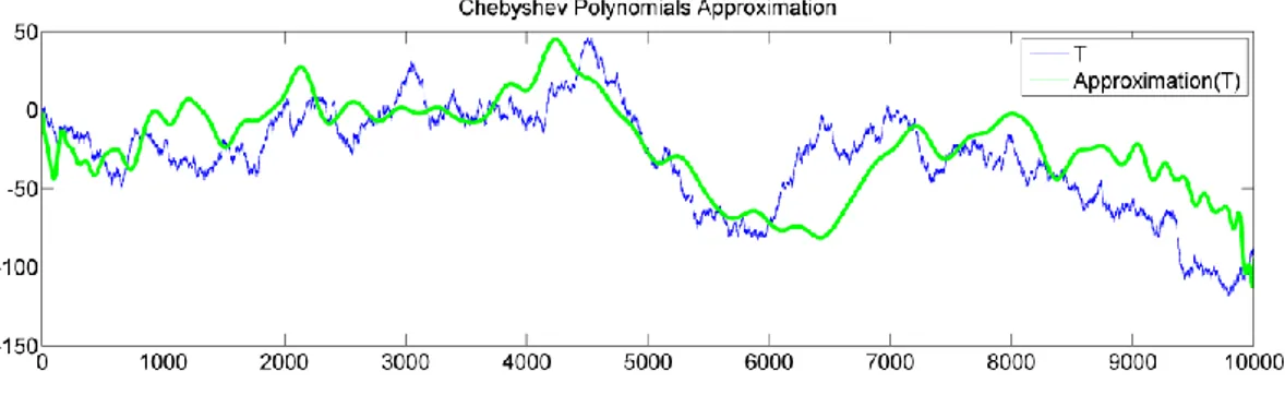
3.7CHEBYSHEV POLYNOMIALS APPROXIMATION... 50

10

CHAPTER 4 - CLASSIFICATION AND PREDICTION ... 55

4.1CLASSIFICATION ... 55

4.1.1 Fisher’s discriminant analysis ... 55

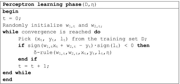
4.1.2 The perceptron criterion function ... 57

4.1.3 k-Nearest Neighbour (kNN) ... 59

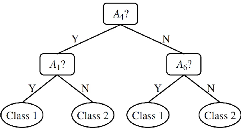
4.1.4 Decision trees ... 59

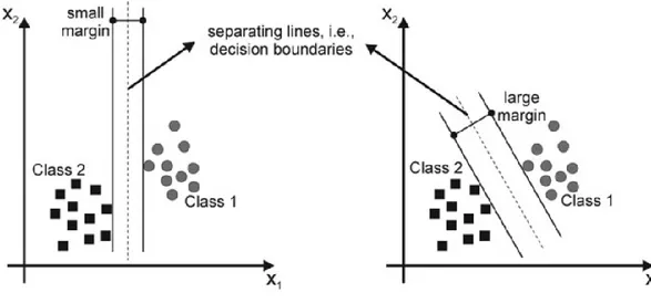
4.1.5 Support Vector Machines (SVMs) ... 61

4.2PREDICTION ... 64

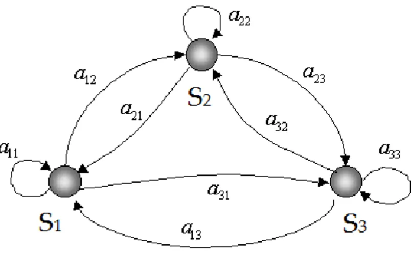
4.2.1 Hidden Markov Models ... 64

Evaluation ... 66 Decoding ... 68 Learning ... 70 CHAPTER 5 - CLUSTERING ... 73 5.1INTRODUCTION ... 73 5.2DEFINITIONS ... 75 5.3CLUSTERING METHODS ... 75 5.3.1. Partitional Clustering ... 77 K-Means ... 78 K-Medoids ... 79 5.3.2. Hierarchical Clustering ... 80 Mean Distance ... 80 Minimum Distance... 81 Maximum Distance ... 81 Average Distance ... 81 BIRCH ... 82 CURE ... 83 ROCK ... 84 CHAMELEON ... 84 5.3.3. Density-based Clustering ... 86 DBSCAN ... 87 OPTICS ... 89 DENCLUE ... 90 5.3.4. Graph-based Clustering ... 93 Node-Centric Community ... 94 Group-Centric Community ... 95 Network-Centric Community ... 95 Hierarchy-Centric Community ... 99 5.3.5 Grid-based Clustering ... 99 STING ... 99 Wavecluster ... 100 5.3.6 Other techniques ... 102

11

Model-based Clustering ... 102

Subspace Clustering ... 103

Neural Network Clustering ... 104

5.3.7 Evaluating clustering ... 107

5.4OUTLIER DETECTION ... 111

5.5ENHANCING DENSITY-BASED CLUSTERING ... 114

5.5.1. Stratification based outlier detection ... 116

5.5.2. Development of a new density-based algorithm ... 120

5.5.3 DBStrata ... 126

CHAPTER 6 - GEOPHYSICAL APPLICATION OF DATA MINING . 131 6.1CLUSTERING AND CLASSIFICATION OF INFRASONIC EVENTS AT MOUNT ETNA USING PATTERN RECOGNITION TECHNIQUES ... 131

6.1.1 Infrasound features at Mt. Etna ... 133

6.1.2 Data acquisition and infrasound signal characterization ... 134

Data acquisition and event detection ... 134

Infrasonic signal features extraction ... 135

Semblance algorithm ... 139

6.1.3 Learning phase ... 139

6.1.4 Testing phase and final system ... 143

6.2CHARACTERIZATION OF PARTICLES SHAPES BY CAMSIZER MEASUREMENTS AND CLUSTER ALGORITHMS ... 146

6.2.1 Definition of the shape ... 147

6.2.2 Methodology ... 150 CAMSIZER ... 151 Features ... 153 6.2.3 Data analysis ... 155 6.2.4 Results ... 157 6.2.5 Future works ... 158

6.3MOTIF DISCOVERY ON SEISMIC AMPLITUDE TIME SERIES: THE CASE STUDY OF MT.ETNA 2011 ERUPTIVE ACTIVITY... 160

6.3.1 Data analysis ... 161

6.3.2 Motif discovery theory ... 162

5.3.3 Results ... 167

5.3.4 Discussion and conclusions ... 175

6.4AN APPLICATION OF SEGMENTATION METHOD ON SEISMO-VOLCANIC TIME SERIES ... 181

6.5MONITORING VOLCANO ACTIVITY THROUGH HIDDEN MARKOV MODEL ... 185

6.5.1 Modelling RMS values distribution ... 185

Distribution fitting ... 186

12

6.5.2 Implementing the framework ... 189

HMM settings ... 191 6.5.3 Classification results ... 192 CONCLUSIONS ... 197 APPENDICES ... 199 A-COVARIANCE MATRIX ... 201 B-SOMPI METHOD ... 203 C-DATA TRANSFORMATION ... 207 D-REGRESSION ... 213

E-DETERMINING THE WIDTH OF HISTOGRAM BARS ... 217

Sturge’s rule ... 217

Scott’s rule ... 217

Freedman – Diaconis rule ... 218

13

Chapter 1

Introduction

Data mining has a very recent origin and has no single definition. Various definitions have been proposed:

"Data mining is the search for relationships and global patterns that exist in large databases, but are ‘hidden’ among the vast amounts of data, such as a relationship between patient data and their medical diagnosis. These relationships represent valuable knowledge about the database and objects in the database and, if the database is a faithful mirror, of the real world registered by the database"

(Holsheimer and Siebes, 1994).

“Data mining is the exploration and analysis, by means of automatic and semi-automatic methods, of large amounts of data in order to discover meaningful patterns and rules” (Berry et al., 1997).

Data mining can be considered as the ‘art’ of knowledge extraction from huge amount of data. The term is often used as a synonym for Knowledge

Discovery in Databases (KDD):

"Knowledge discovery is the nontrivial extraction of implicit, previously unknown, and potentially useful information from data" (Frawley et al., 1992).

It would be more accurate to speak of knowledge discovery when referring to the process of knowledge extraction, and data mining as a particular phase of this process, consisting in the application of specific algorithms for the identification of "patterns" (Fayyad et al., 1996).

For example, in an industrial or operative domain, useful knowledge is hidden but relevant information. Today the main problem of analysts is to be capable to properly extract the wealth of information which is intrinsically present in the data. Starting from the Fayyad et al. (1996)

14

considerations, the extraction process consists of several phases, each of which brings its rate of information (Figure 1.1): selection from raw data; pre-processing; transformation; application of algorithms for patterns search (in this context a "pattern" means a structure, a model, or, in general, a synthetic representation of the data), followed by their interpretation and evaluation. The identified patterns can be considered, in turn, the starting point to speculate and to verify new relationships among phenomena. They also can be useful to make predictions on new data sets.

Fig. 1.1. General schema of Knowledge Discovery in Database (KDD) process (redrawn from Fayyad et al., 1996).

Data mining is a multidisciplinary field which borrows algorithms and techniques from many research areas such as: machine learning, statistics, neural networks, artificial intelligence, high performance computing technology, database technology, data visualization techniques. The main factors contributing to data mining progress are: the increasing of electronic data, the cheap data storage, and new techniques for analysis (machine learning, pattern recognition).

Algorithms are pillars of data mining techniques, and have to guarantee the effectiveness and efficiency of analysis. Scalability is a fundamental property, because data mining deals with huge amounts of data, and

15

algorithms’ implementation must provide high speed computation, faster than manual data analysis. The execution time of a data mining algorithm must be at least predictable and acceptable according to the size of the analyzed database. Data mining algorithms have to adapt to the hardware advances, trying to properly exploit its potential, such as the computing on multiple processors (parallel or distributed computing), and then afford the problems inherent to the database size.

Data mining is an interdisciplinary branch of the science which takes its origins in statistics. The reason behind the wide usage of data mining techniques relies on its simplicity (w.r.t. classical statistical methods), its scalability and its wide range application domains. In principle any kind of data can be analyzed with proper mining technique. However, data mining has similar limits to all statistical approaches, such as the GIGO (Garbage In, Garbage Out): if the input is “garbage”, then the output will be “garbage”. Thus, the optimal strategy is to use statistics and data mining as two complementary approaches.

The data mining techniques can be divided into two broad categories: supervised and unsupervised learning techniques.

The supervised learning aims to realize a computer system able to automatically solving a specific trained problem. In order to produce a generalized model for the problem, a supervised learning algorithm makes use of some examples, in particular: (i) it defines a set of input data

I; (ii) it defines a range of output values O; (iii) and defines a function h

that maps each input data to correct output value. Providing a large number of examples, the algorithm of supervised learning will be able to identify a new function h1 that will approximate the function h. Of course,

the goodness of the algorithm depends on the dataset used in the training phase. In fact, it has to avoid the "overtraining" on input: a model is considered to be good if it is able to predict the output of never learned data, only with the knowledge provided by the input. It may happen in fact that the model specializes only on the recognition of the sample of the input data, producing the “overfitting” problem. Through the supervised learning, data mining is able to face problems concerning: (i) classification operations, where observations are "labeled" (or associated to a class) on the basis of well-known characteristics of the class; (ii) model estimation, such as to see whether the distribution of an observation follows a

16

statistical known model, such as the Gaussian distribution; (iii) attempt to identify future trends (prediction) of an observed variable or characteristic.

The unsupervised learning builds models without apriori knowledge. Different from supervised learning, in the learning phase, the labels or the model of the examples are not provided. The algorithms are based on comparisons between data and the search for similarities and differences. In this contest can be realized: (i) operations of grouping (or clustering), by finding homogeneous groups that present characteristical regularities within them and differences among groups (clusters); (ii) association rules, which identify any associations between data. These last are widely applied in the transactional database to find relationships between products purchased together, as in the case of the market basket analysis, to implement marketing strategies, such as promotional offers, or the positioning of the products on the shelves.

1.1 Typical data mining tasks

Given a collection of objects, a database D, most of data mining research is related to the similarity matching problem, including the following tasks:  Indexing: given a query object Q, and a similarity/dissimilarity

measure dist(o,p) defined for  ,o pD, it consists on building a data structure, allowing speed-up search of the nearest neighbor of Q in D. There are two ways to post a similarity query [3]:

 k-nearest neighbors: dealing with the search of the set of first k objects D more similar to Q.

 range query: finds the set R D of objects that are within distance r from Q.

 Clustering: consists of division of data into groups (clusters) of similar objects under some similarity/dissimilarity measure. The search for clusters is unsupervised. It is often complementary to the anomaly/outlier detection problem, which seeks for objects showing different attributes respect to the whole dataset.

17

 Classification: assigns unlabeled objects to predefined classes after a supervised learning process, based on classes properties.

1.2 Time series data mining

In the last years, there has been an increasing interest in methods dealing with time series data. It depended on the rapid growth of generated daily information from several areas, e.g., finance, computational biology, sensor networks, location-based services, etc. A time series is “a sequence X

= (x1, x2, …, xm) of observed data over time”, where m is the number of

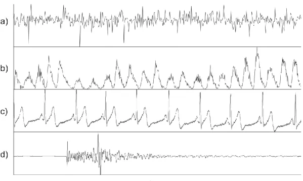
observations. Tracking the behavior of a specific phenomenon/data in time can produce important information (Fig. 1.2). A large variety of real world applications, such as meteorology, geophysics and astrophysics, collect observations that can be represented as time series.

Fig. 1.2. Examples of time series data relative to a) monsoon, b) sunspots, c) ECG (ElectroCardioGram), d) seismic signal.

18

Often in time series data mining these other two following tasks are relevant:

 Summarization: given a raw time series Q of length m, makes a new time series representation Q’ lighter than Q (with length m’ < m) in term of space, that approximate Q fitness. This task is very important to achieve the best performances on previous tasks.

 Prediction: finds a model for the sequence of observations, to check dependencies among them, and then predict a future value. While in the classification task an observation is assigned to a specific class, providing an output of categorical, the prediction task provides a specific observation value. It can be also used to replace missing values on data.

1.3 Data mining on geophysics

The geophysical data are automatically measured and recorded by geophysical instruments. Their interpretation is very important for the investigation of earth’s behavior. Generally, the amount of data is very large and relatively standard. It is suitable to be processed and be analyzed by data mining techniques. The analysis can be conducted on real time data, or on historical data.

The former task is the most interesting type of analysis, because permits to monitor alert situations and to prevent most of human risks: this thesis focuses on volcano monitoring. The latter task often consists of extracting previously unknown recurrent patterns from available data, and constitutes a crucial step in geophysical time series analysis, because allow to increment the suitable amount of information for the monitoring task.

19

Chapter 2

Fundamentals on similarity matching

In data mining, several terms are used to refer to a single data into database: object, point, record, observation, item or tuple. In this chapter, we will use the term object to denote a single element of a dataset. In multi-dimensional spaces, an object is described by a number of components or

features, which we will refer as attributes.

More formally, a dataset with N objects, each of which is described by m attributes, is denoted by D = {x1, x2, . . . , xN}, where xi = (xi(1), xi(2), . . . , xi(m)) is

a vector denoting the ith object and xi(j) is a value denoting the jth attribute

of xi. The number of attributes m indicates the dimensionality of the data

set. The general representation of such data is a matrix N × m used by most of the algorithms described below.

                     ) ( ) ( ) ( ) ( ) ( ) ( ) ( ) ( ) ( ) ( ) ( ) ( ) ( ) ( ) ( ) ( m N j N N N m i j i i i m j m j x x x x x x x x x x x x x x x x D                     2 1 2 1 2 2 2 2 1 2 1 1 2 1 1 1 (2.1)

2.1 Types of data

Data mining algorithms strongly depend on attributes of managed data types. A basic classification distinguishes two main categories of attributes: quantitative and qualitative. Quantitative attributes come from numeric measurements, and can represent continuous values (e.g. height), and discrete values (e.g. number of children). For quantitative attribute, there is another distinction between interval attributes, where measurements are disposed on a linear scale, and ratio attributes, which are disposed on a nonlinear scale.

20

Qualitative attributes come from previously established categories, and can be categorical (or nominal; e.g. eye’s color), binary (e.g. sex), and ordinal (e.g. military rank). Binary attribute is a special case of categorical attribute taking exactly two categories: it is possible to give same weight for both categories (symmetric) or not (asymmetric). It is possible to realize a map from interval to ordinal and nominal attributes, or from ordinal to nominal, and vice-versa (Gan et al., 2007).

In the real world, however, there exist various other data types, such as image data, graph, or time series containing, in turn, quantitative and/or qualitative data.

2.2 Indexing

In many cases, datasets are supported by special data structures, especially when dataset get larger, that are referred as indexing structures. Indexing consists of building a data structure I that enables efficient searching within database (Ng and Cai, 2004). Usually, it is designed to face two principal similarity queries: the (i) k-nearest neighbors (knn), and the (ii) range query problem. Given a query object Q in D, and a similarity/dissimilarity measure d(x,y) defined for each pair x, y in D, the former query deals with the search of the set of first k objects in D more similar to Q. The latter query finds the set R of objects that are within distance r from Q. When dealing with a collection of time series, a TSDB (Time Series DataBase), given an indexing structure I, there are two ways to post a similarity query (Ng and Cai, 2004):

 whole matching: given a TSDB of time series, each of length m, whole matching relates to computation of similarity matching among time series along their whole length.

 subsequence matching: given a TSDB of N time series S1, S2, …, SN, each of

length mi, and a short query time series Q of length mq < mi, with 0 < i <

N, subsequence matching relates to finding matches of Q into

21

Indexing is crucial for reaching efficiency on data mining tasks, such as

clustering or classification, especially for huge database such as TSDBs.

Clustering is related to the unsupervised division of data into groups (clusters) of similar objects under some similarity or dissimilarity (distances) measures. Sometimes, on time series domain, a similar problem to clustering is the motif discovery problem (Mueen et al., 2009), consisting of searching main cluster (or motif) into a TSDB. The search for clusters is unsupervised. Classification assigns unlabeled objects to predefined classes after a supervised learning process. Both tasks make massive use of distance computations.

Distance measures play an important role in similarity matching problem. Concerning a distance measure, it is important to understand if it can be considered metric function. A metric function on a set D is a function

f : D × D → R (where R is the set of real numbers). For all x, y, z in D, this

function obeys to four fundamental properties:

1. f(x, y) ≥ 0 (non-negativity) (2.2)

2. f(x, y) = 0 if and only if x = y (identity) (2.3)

3. f(x, y) = f(y, x) (symmetry) (2.4)

4. f(x, z) ≤ f(x, y) + f(y, z) (triangle inequality) (2.5) If any of these is not obeyed, the distance is considered non-metric. Using a metric function is desired, because the triangle inequality property (Eq. 2.5) can be used to perform the indexing of the space for speed-up search in large datasets. By means of adequate indexing data structures (general tree structures) such as kd-tree (Bentley, 1975), R* tree (Beckmann et al., 1990), or Antipole tree (Cantone et al., 2005), it is possible to perform pruning during search on the space. Best efforts have been devoted to similarity searching, with emphasis on metric space searching. In this sense SISAP, a conference devoted to similarity searching (http://sisap.org/Home.html) provides the Metric Space Library

(http://sisap.org/Metric_Space_Library.html) allowing to use a wide range of indexing techniques for general spaces (metric and non-metric). Another well known framework for indexing, overall for multimedia and time series data, is GEMINI (GEneric Multimedia INdexIng; Faloutsos et al.,

22

1994), that designs fast search algorithms for locating objects series that match, in an exact or approximate way, a query time series Q.

Algorithms dealing with relative small datasets mostly use a simple data structure, an N × N matrix, called also distance matrix, proximity matrix, or

affinity matrix, storing distances between each pair of dataset objects:

                     0 ) 1 , ( ) 2 , ( ) 1 , ( 0 0 ) 2 , 3 ( ) 1 , 3 ( 0 ) 1 , 2 ( 0 N N d N d N d d d d distMatrix           _(2.6)

where d(i,j) indicates distance between ith and jth object (for 0 < i, j < N). For metric distance functions, the matrix is symmetric, because of the metric symmetric property (Eq. 2.4), and all diagonal elements have zero values, since d(i,i) = 0 for the identity property (Eq. 2.3). If we store similarity measures instead of distances the resulting matrix will be called

similarity matrix.

2.3 Similarity and Distance Measures

A common data mining task is the estimation of similarity among objects. A similarity measure is a relation between a pair of objects and a scalar number. In this subsection some of the common distance measures, used for numerical data and not, are formally described. Let be two objects X and Y of m attributes, and xi and yi the ith attributes of X and Y,

respectively. Let us list the following measures.

2.3.1 Numerical Similarity Measures

Common intervals used to mapping the similarity are [-1, 1] or [0, 1], where 1 indicates the maximum of similarity.

Considering the similarity between two attributes xi and yi as :

i i i i i i

y

x

y

x

y

x

numSim







1

)

,

(

23 Mean Similarity



Root Mean Square Similarity:





y

x

numSim

m

Y

X

rtsim

)

,

(

1

)

,

(

Peak similarity (Fink and Pratt, 2004):





























y

x

y

x

m

Y

X

psim

2

max

,

1

1

)

,

(

Cosine similarity. In some applications, such as information retrieval, text

document clustering, and biological taxonomy, it is possible that the measures mentioned above are not used. Often, when dealing with vector objects, the most used distance function is the cosine similarity.

The cosine similarity computes the cosine of the angle θ between two objects X and Y, and is defines as:

 

 

_

 







y

x

y

x

cos



This measure provides values in range [-1, 1]. The lower boundary indicates that the X and Y vectors are exactly opposite; the upper boundary indicates that the vectors are exactly the same; finally the 0 value indicates the independence.

Cross-correlation. Another common similarity function used to perform

complete or partial matching between time series is the cross-correlation function (or Pearson’s correlation function) (Von Storch and Zwiers, 2001).

24

The cross correlation between two time series X and Y of length m, allowing a shifted comparison of l positions, is defined as:











_









where X and Y are the means of X and Y. The correlation rXY provides

the degree of linear dependence between the two vectors X and Y from perfect linear relationship (rXY = 1), to perfect negative linear relation (rXY =

-1).

2.3.2 Numerical Distance Measures

Euclidean Distance. The most used distance function in many

applications. It is defined as: 2 1 1 2 ) ( ) , ( _      _ 



Manhattan Distance. Also called “city block distance”. It is defined as:



Maximum Distance. It is defined to be the maximum value of the

distances of the attributes:

i i m i x y Y X d     0 max ) , ( (2.15)

Minkowski Distance. The Euclidean distance (Eq. 2.13), Manhattan distance

(Eq. 2.14), and Maximum distance (Eq. 2.15), are particular instances of the

Minkowski distance, called also Lp-norm. It is defined as:

p m i p i i y x Y X d 1 1 ) ( ) , ( _       



25

where p is called the order of Minkowski distance. In fact, for Manhattan distance p = 1, for the Euclidean distance p = 2, while for the Maximum distance p = ∞.

Mahalanobis Distance. The Mahalanobis distance is defined as:



 



where Σ is the covariance matrix (see Appendix A, Eq. A.3; Duda et al., 2001).

2.3.3 Binary and Categorical Data Measures

Binary data can have only two values: 0 and 1 (or true and false, positive and negative). To compute distance between two data objects X, Y, containing m binary attributes, it is usual to fill a 2 × 2 matrix T, called

contingence table, which contains all possible test results:

             Y m t r s q sum t s t s r q r q sum X T                         0 1 0 1 (2.18)

where q is the number of attributes that equal 1 for both objects X and Y, r is the number of attributes that equal 1 for object X but that are 0 for object

Y, s is the number of attributes that equal 0 for object X but equal 1 for

object Y, and t is the number of attributes that equal 0 for both objects X and Y.

For symmetric binary data, where both values have the same weight, it is used a very common distance function, defined as:

m s r t s r q s r Y X d        ) , ( (2.19)

26

For asymmetric binary data, by convention, 1 is associated to the weight having more importance. This criterion has most application in medical tests for diseases: positive test, the rarest, have greater significance than negative test. So, it is usual to assign 1 to positive test and 0 to negative test. t, in this case, is considered unimportant, and thus is ignored in the computation of the following distance function:

s r q s r Y X d     ) , ( (2.20)

This distance function is often known as Jaccard distance (Han and Kamber, 2000).

Categorical data are a generalization of binary data. Let r and s be two categories of categorical data. A matching between these two categories can be defined in this simple way:

      s r s r s r 1 0 ) , (  (2.21)

The Simple Matching distance for two categorical data X and Y, described by m attributes, can be defined as:



where xi and yi corresponding to the ith attributes of X and Y, respectively.

2.3.4 Measures for Time Series Data

A time series is a sequence of real numbers representing measurements over time. When treating time series, the similarity between two sequences of the same length can be calculated by summing the ordered

point-to-point distance between them (Fig. 2.1), where “point” stays for a

27

Fig. 2.1. x and y are two time series of a particular variable v, along the time axis t. The Euclidean distance results the sum of the point-to-point distances (gray lines), along all the time series.

In this sense, the most used distance function is the Euclidean distance (Faloutsos et al., 1994), corresponding to the second degree of general Lp

-norm. This distance measure is cataloged as a metric distance function,

since it obeys to the metric properties: non-negativity, identity, symmetry and triangle inequality (Eq. 2.3~2.5). Euclidean distance is surprisingly competitive with other more complex approaches, especially when dataset size gets larger (Shieh and Keogh, 2008). In every way, Euclidean distance and its variants present several drawbacks, which make inappropriate their use in certain applications:

 It compares only time series of the same length.  It cannot handle outliers or noise.

 It is very sensitive respect to six signal transformations: shifting, uniform amplitude scaling, uniform time scaling, uniform bi-scaling, time warping and non-uniform amplitude scaling (Perng et al., 2000). For these reasons, other distance measure techniques were proposed to give more robustness to the similarity computation. In this sense it is required to cite also the well known Dynamic Time Warping (DTW; Keogh and Ratanamahatana, 2002) taking advantage of dynamic programming to allow comparison of one-to-many points; and the Longest Common

28

dynamic programming solution as DTW, but more resilient to noise. In the literature there exist other distance measures that overcome signal transformation problems, such as the Landmarks similarity, which does not follow traditional similarity models that rely on point-wise Euclidean distance (Perng et al., 2000) but, in correspondence of human intuition and episodic memory, relies on similarity of those points (times, events) of “greatest importance” (for example local maxima, local minima, inflection points). Unfortunately, none of them is metric, so they cannot take advantage of any indexing structure.

Dynamic Time Warping. Dynamic Time Warping (Berndt and Clifford,

1994) gives more robustness to the similarity computation. By this method, also time series of different length can be compared, because it replaces the one-to-one point comparison, used in Euclidean distance, with a many-to-one (and viceversa) comparison. The main feature of this distance measure is that it allows recognizing similar shapes, even if they present signal transformations, such as shifting and/or scaling (Fig. 2.2). Given two time series T = {t1, t2, . . . , tn} and S = {s1, s2, . . . , sm} of length n

and m, respectively, an alignment by DTW method exploits information contained in an n × m distance matrix:

             ) , ( ) , ( ) , ( ) , ( ) , ( ) , ( ) , ( 1 2 2 1 2 1 2 1 1 1 m n n m S T d S T d S T d S T d S T d S T d S T d distMatrix    (2.23)

where distMatrix(i, j) corresponds to the distance of ith point of T and jth point of S d(Ti, Sj), with 1 ≤ i ≤ n and 1 ≤ j ≤ m.

The DTW objective is to find the warping path W = {w1, w2, . . . ,wk, . . ., wK} of

contiguous elements on distMatrix (with max(n, m) < K < m + n -1, and wk =

distMatrix(i, j)), such that it minimizes the following function:

      



29

Fig. 2.2. Difference between DTW distance and Euclidean distance (green lines represent mapping between points of time series T and S). The former allows many-to-one point comparisons, while Euclidean point-to-point distance (or many-to-one-to-many-to-one).

The warping path is subject to several constraints (Keogh and Ratanamahatana, 2002). Given wk = (i, j) and wk-1 = (i’, j’) with i, i’ ≤ n and j,

j’ ≤ m :

1. Boundary conditions. w1 = (1,1) and wK = (n, m).

2. Continuity. i – i’ ≤ 1 and j – j’ ≤ 1. 3. Monotonicity. i – i’ ≥ 0 and j – j’ ≥ 0.

The warping path can be efficiently computed using dynamic programming (Cormen et al. 1990). By this method, a cumulative distance matrix γ of the same dimension as the distMatrix, is created to store in the cell (i, j) the following value (Fig. 2.3):





30

Fig. 2.3. Warping path computation using dynamic programming. The lavender cells correspond to the warping path. The red arrow indicates its direction. The warping distance at the (i, j) cell will consider, besides the distance between Ti and Sj, the

minimum value among adjacent cells at positions: (i-1, j-1), (i-1, j) and (i, j-1). The Euclidean distance between two time series can be seen as a special case of DTW, where path’s elements belong to the γ matrix diagonal.

The overall complexity of the method is relative to the computation of all distances in distMatrix that is O (nm). The last element of the warping path, wK corresponds to the distance calculated with the DTW method.

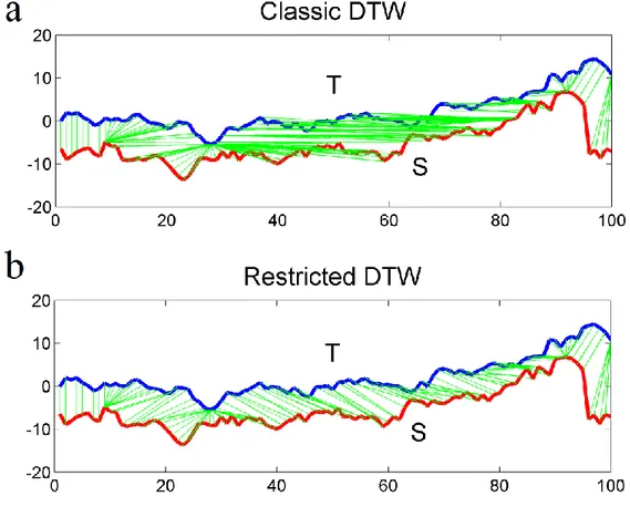
In many cases, this method can bring to undesired effects. An example is when a large number of points of a time series T are mapped to a single point of another time series S (Fig. 2.4a, 2.5a). A common way to overcome this problem is to restrict the warping path in such a way it has to follow a direction along the diagonal (Fig. 2.4b, 2.5b). To do this, we can restrict the path enforcing the recursion to stop at a certain depth, represented by a threshold δ. Then, the cumulative distance matrix γ will be calculated as follows:





Figure 2.5a shows the computation of a restricted warping path, using a threshold δ = 10. This constraint, besides limiting extreme or degenerate mappings, allows to speed-up DTW distance calculation, because we need to store only distances which are at most δ positions away (in horizontal

31

and vertical direction) from the distMatrix diagonal. This reduces the computational complexity to O((n + m)δ). The above proposed constraint is known also as Sakoe-Chiba band (Fig. 2.6a; Sakoe and Chiba, 1978) , and it is classified as global constraint. Another most common global constraint is the Itakura parallelogram (Fig. 2.6b; Itakura, 1975).

Fig. 2.4. Different mappings obtained with the classic implementation of DTW (a), and with the restricted path version using a threshold δ = 10 (b). Green lines represent mapping between points of time series T and S.

Local constraints are subject of research and are different from global constraints (Keogh and Ratanamahatana, 2002), because they provide local restrictions on the set of the alternative depth steps of the recurrence function (Eq. 2.25). For example we can replace Eq. 2.25 with:





32

Fig. 2.5. (a) Classic implementation of DTW. (b) Restricted path, using a threshold δ = 10. For each plot (a) and (b): on the center, the warping path calculated on matrix γ. On the top, the alignment of time series T and S, represented by the green lines. On the left, the time series T. On the bottom, the time series S. On the right, the color bar relative to the distance values into matrix γ.

33

Fig. 2.6. Examples of global constraints: (a) Sakoe-Chiba band; (b) Itakura parallelogram.

Longest Common SubSequence. Another well known method that takes

advantage of dynamic programming to allow comparison of one-to-many points is the Longest Common SubSequence (LCSS) similarity measure (Vlachos et al., 2002). An interesting feature of this method is that it is more resilient to noise than DTW, because allows some elements of time series to be unmatched (Fig. 2.7). This solution builds a matrix LCSS similar to γ, but considering similarity instead of distances.

Given the time series T and S of length n and m, respectively, the recurrence function is expressed as follows:

 

with 1 ≤ i ≤ n and 1 ≤ j ≤ m. Since exact matching between Ti and Sj can be

strict for numerical values (Eq. 3.22 is best indicated for string distance computation, such as the edit distance), a common way to relax this definition is to apply the following recurrence function:

 

The cell LCSS(n, m) contains the similarity between T and S, because it corresponds to length l of the longest common subsequence of elements

34

between time series T and S. To define a distance measure, we can compute (Ratanamahatana et al., 2010):

n m l m n S T LCSSdist     2 ) , ( (2.30)

Also for LCSS the time complexity is O(nm), but it can be improved to

O((n + m)δ) if a restriction is used (i.e. when |i - j| < δ).

Fig. 2.7. Alignment using LCSS. Time series T (red line) is obtained from S (blue line), by adding a fixed value = 5, and further “noise” at positions starting from 20 to 30. In these positions there is no mapping (green lines).

35

Chapter 3

Dimensionality reduction techniques

Time series are often high dimensional data objects, thus dealing directly with the raw representation can be expensive in terms of space and time. In this sense, an important aspect to achieve efficiency, by means of space compression, is the use of dimensionality reduction techniques; while effective querying on time series data can be reached by using adequate similarity measures and space indexing. The goal of this chapter is to provide an overview of main dimensionality reduction algorithms (Cassisi et al., 2012c). Mining high-dimensional involves addressing a range of challenges, among them: i) the curse of dimensionality (Agrawal et al., 1993), and ii) the meaningfulness of the similarity measure in the high-dimensional space. A key aspect to achieve efficiency, when mining time series data, is to work with a data representation that is lighter than the raw data. This can be done by reducing the dimensionality of data, still maintaining its main properties. An important feature to be considered, when choosing a representation, is the lower bounding property.

Given two raw representations of the time series T and S, by this property, after establishing a true distance measure dtrue for the raw data (such as the

Euclidean distance), the distance dfeature between two time series, in the

reduced space, R(T) and R(S), have to be always less or equal than dtrue:

) , ( )) ( ), ( (RT RS d T S d_feature  _true (3.1)

If dimensionality reduction techniques ensure that the reduced representation of a time series satisfies such a property, we can assume that the similarity matching in the reduced space maintains its meaning. Moreover, we can take advantage of indexing structure such as GEMINI (Section 2.2) to perform speed-up search even avoiding false negative results. GEMINI was introduced to accommodate any dimensionality reduction method for time series, and then allows indexing on new

36

representation (Ng and Cai, 2004). GEMINI guarantees no false negatives on index search if two conditions are satisfied: (i) for the raw time series, a metric distance measure must be established; (ii) to work with the reduced representation, a specific requirement is that it guarantees the lower

bounding property. In the following subsections, we will review the main

dimensionality reduction techniques that preserve the lower bounding property. By this property, after establishing a true distance measure for the raw data (in this case the Euclidean distance), the distance between two time series, in the reduced space, results always less or equal than the true distance. Such a property ensures exact indexing of data (i.e. with no false negatives). The following representations describe the state-of-art in this field: spectral decomposition through Discrete Fourier Transform (DFT) (Agrawal et al., 1993); Singular Value Decomposition (SVD) (Korn et al., 1997); Discrete Wavelet Transform (DWT) (Chan and Fu, 1999); Piecewise

Aggregate Approximation (PAA) (Keogh et al., 2000); Piecewise Linear Approximation (PLA) (Keogh et al., 2001); Adaptive Piecewise Constant Approximation (APCA) (Chakrabarti et al., 2002); and Chebyshev Polynomials

(CHEB) (Ng and Cai, 2004). Many researchers have also included symbolic representations of time series, that transform time series measurements into a collection of discretized symbols; among them we cite the Symbolic

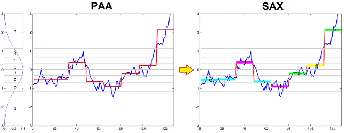
Aggregate approXimation (SAX) (Lin et al., 2007), based on PAA, and the

evolved multi-resolution representation iSAX 2.0 (Shieh and Keogh, 2008). Symbolic representation can take advantage of efforts conducted by the text-processing and bioinformatics communities, who made available several data structures and algorithms for efficient pattern discovery on symbolic encodings (Lawrence et al., 1993; Bailey and Elkan, 1995; Tompa and Buhler, 2001).

3.1 DFT

The dimensionality reduction, based on the Discrete Fourier Transform (DFT) (Agrawal et al., 1993), was the first to be proposed for time series. The DFT decomposes a signal into a sum of sine and cosine waves, called

Fourier Series. Each wave is represented by a complex number known as Fourier coefficient (Fig. 3.1) (Ng and Cai, 2004; Ratanamahatana et al., 2010).

37

because the original signal can be reconstructed by means of information carried by the waves with higher Fourier coefficient. The rest can be discarded with no significant loss.

Fig. 3.1. The raw data is in the top-left plot. In the first row, the central plot (“Fourier coefficients” plot) shows the magnitude for each wave (Fourier coefficient). Yellow points are drawn for the top ten highest values. The remaining plots (in order from first row to last, and from left to right) represent the waves corresponding to the top ten highest coefficients in decreasing order, respectively of index {2, 100, 3, 99, 98, 4, 93, 9, 1, 97}, in the “Fourier coefficients” plot.

More formally, given a signal x = {x1, x2, . . . , xn}, the n-point Discrete

Fourier Transform of x is a sequence X = {X1, X2, . . . , Xn} of complex

numbers. X is the representation of x in the frequency domain. Each wave/frequency XF is calculated as:

n F j e x n X n i n ijF i F ( 1) 1, , 1 1 2     



38

The original representation of x, in the time domain, can be recovered by the inverse function:

n i j e X n x n F n ijF F i ( 1) 1, , 1 1 2     



The energy E(x) of a signal x is given by:



A fundamental property of DFT is guaranteed by the Parseval’s Theorem, which asserts that the energy calculated on time series domain for signal x is preserved on frequency domain, and then:

) ( ) ( 1 2 1 2 X E X x x E n F F n i i   





If we use the Euclidean distance (Eq. 2.13), by this property, the distance

d(x,y) between two signals x and y on time domain is the same as

calculated in the frequency domain d(X,Y), where X and Y are the respective transforms of x and y. The reduced representation X’ = {X1, X2, .

. . , Xk} is built by only keeping first k coefficients of X to reconstruct the

signal x (Fig. 3.2).

For the Parseval’s Theorem we can be sure that the distance calculated on the reduced space is always less than the distance calculated on the original space, because k ≤ n and then the distance measured using Eq. 2.13 will produce: ) , ( ) , ( ) ' , ' (X Y d X Y d x y d   (3.6)

that satisfies the lower bounding property defined in Eq. 3.1.

The computational complexity of DFT is O(n2_{), but it can be reduced by}

means of the FFT algorithm (Cooley and Tukey, 1965), which computes the DFT in O(n log n) time. The main drawback of DFT reduction

39

technique is the choice of the best number of coefficients to keep for a faithfully reconstruction of the original signal.

Fig. 3.2. The raw data is in the top-left plot. In the first row, the central plot (“Fourier coefficients” plot) shows the magnitude (Fourier coefficient) for each wave. Yellow points are drawn for the top ten highest values. The remaining plots (in order from first row to last, and from left to right) represent the reconstruction of the raw data using the wave with highest values (of index 2) firstly, then by adding the wave relative to second highest coefficient (of index 100), and so on.

3.2 DWT

Another technique for decomposing signals is the Wavelet Transform (WT). The basic idea of WT is data representation in terms of sum and difference of prototype functions, called wavelets. The discrete version of WT is the

Discrete Wavelet Transform (DWT). Similarly to DFT, wavelet coefficients

40

coefficients always represent global contributions to the signal over all the time (Ratanamahatana et al., 2010).

The Haar wavelet is the simplest possible wavelet. Its formal definition is given by Chan and Fu (1999). An example of DWT based on Haar wavelet is shown in Table 3.1. The general Haar transform HL(T) of a time series T

of length n can be formalized as follows:

2 ) 1 2 ( ) 2 ( ) ( ' ' 1 '     i A i A i A_L L L (3.7) 2 ) 1 2 ( ) 2 ( ) ( ' ' 1 '     i D i D i D_L L L (3.8) ) , , , , ( ) ( _{L L L 1 o} L T A D D D H  _  (3.9) where 0 < L’ ≤ L, and 1 ≤ i ≤ n.

Level (L) Averages coefficients (A) Wavelet coefficients (D)

1 10, 4, 6, 6

2 8, 6 3, 0

3 7 1

Table 3.1. The Haar transform of T = {10, 4, 8, 6} depends on the chosen level, and corresponds to merging Averages coefficients (column 2) at the chosen level and all Wavelet coefficients (column 3) in decreasing order from the chosen level. At level 1 the representation is the same of time series: H1(T) = {10, 4, 6, 6} + {} = {10, 4, 6, 6} = T. At level 2 is H2(T) = {8, 6} + {3, 0} + {} = {8, 6, 3, 0}. At level 3 is H3(T) = {7} + {1} + {3, 0} = {7, 1, 3 0}.

The main drawback of this method is that it is well defined for time series which length n is a power of 2 (n = 2m_{). The computational complexity of}

DWT using Haar Wavelet is O(n).

Chan and Fu (1999) demonstrated that the Euclidean distance between two time series T and S, d(T,S), can be calculated in terms of their Haar transform d(H(T), H(S)), by preserving the lower bounding property in Eq. 3.1, because: ) , ( ) , ( 2 )) ( ), ( (H T H S dT S dT S d   (3.10)

41

Fig. 3.3. DWT using Haar Wavelet with MATLAB Wavelet Toolbox™ GUI tools. T is a time series of length n = 256 and it is shown on the top-left plot (Original Signal). On the bottom-left plot (Original Coefficients) there are the entire AL, represented by blue

stems, and DL’ coefficients (L’ < L = 7), represented by green stems (stems’ length is

proportional to coefficients value). On the top-right plot, the Synthesized Signal by selecting only the 64 biggest coefficients, as reported on the bottom-right plot (Selected

Coefficients): black points represent unselected coefficients.

3.3 SVD

As we have just seen in Chapter 2, a dataset with m time series (TSDB), each of length n, can be represented by an m × n matrix D (Eq. 2.1). An important result from linear algebra is that D can always be written in the form (Golub and Van Loan, 1996):

T

UWV

D  (3.11)

where U is an m × n matrix, W and V are n × n matrices. This is called the

Singular Value Decomposition (SVD) of the matrix D, and the elements of the n × n diagonal matrix W are the singular values wi:

42              n w w w W        0 0 0 0 0 0 2 1 (3.12)

V is orthonormal, because VVT _{= V}T_{V = In, where In is the identity matrix of}

size n. So, we can multiply both sides of Eq. 3.11 by V to get:

UW AV V

UWV

AV  T   _(3.13)

UW represents a set of n-dimensional vectors AV ={X1, X2, . . . , Xm} which

are rotated from the original vectors A={x1, x2, . . . , xm} (Ng and Cai, 2004):

                                     n m m w w w U U U X X X          0 0 0 0 0 0 2 1 2 1 2 1 (3.14)

Similarly to sine/cosine waves for DFT (Section 3.1) and to wavelet for

DWT (Section 3.2), U vectors represent basis for AV, and their linear

combination with W (that represents their coefficients) can reconstruct AV. We can perform dimensionality reduction by selecting the first ordered k biggest singular values and their relative entries in A, V and U, to obtain a new k-dimensional dataset that best fits original data (Fig. 3.4).

SVD is an optimal transform if we aim to reconstruct data, because it

minimizes the reconstruction error, but have two important drawbacks: (i) it needs a collection of time series to perform dimensionality reduction (it cannot operate on singular time series), because examines the whole dataset prior to transform. Moreover, the computational complexity is

O(min(m2_{n, mn}2_{)). (ii) This transformation is not incremental, because a}

43

Fig. 3.4. SVD for a TSDB of m=7 time series of length n=50. It is possible to note in the

transformed data plot how only first k < 10 singular values are significant. In this

example we heuristically choose to store only first k=5 diagonal elements of V, and their relative entries in A, U and W, because they represent about 95% of total variance. This allows reducing space complexity from n to k, still maintaining almost unchanged the information (see the reconstruction on the bottom-left plot).

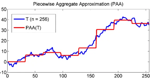
3.4 Dimensionality reduction via PAA

Given a time series T of length n, PAA divides it into w equal sized segments ti (1 < i ≤ w) and records values corresponding to the mean of

each segment mean(ti) (Fig. 3.5) into a vector PAA(T) = {mean(t1), mean(t2),

…, mean(tw)}, using the following formula:



When n is a power of 2, each mean(ti) essentially represents an Averages

coefficient AL(i), defined in Section 3.2, and w corresponds in this case to:

L

n w

2

44

Fig. 3.5. An approximation via PAA technique of a time series T of length n = 256, with

w = 8 segments.

The complexity time to calculate the mean values of Eq. 3.15 is O(n). The

PAA method is very simple and intuitive, moreover it is strongly

competitive with other more sophisticated transforms such as DFT and

DWT (Keogh and Kasetty, 2002; Yi and Faloutsos, 2000). Most of data

mining researches make use of PAA reduction for its simplicity. It is simple to demonstrate how the distance on raw representation is bounded below by the distances calculated on PAA representation (even using Euclidean distance as reference point), satisfying Eq. 3.1. A limitation of such a reduction, in some contexts, can be the fixed size of the obtained segments.

3.5 APCA

In Section 3.2 we noticed that not all Haar coefficients in DWT are important for the time series reconstruction. Same thing for PAA in Section 3.4, where not all segment means are equally important for the reconstruction, or better, we sometimes need an approximation with no-fixed size segments. APCA is an adaptive model that, differently from

PAA, allows defining segments of variable size. This can be useful when

45

which we want to have, respectively, few segments for the former, and many segments for the latter.

Given a time series T = {t1, t2, . . . , tn} of length n, the APCA representation

of T is defined as (Chakrabarti et al., 2002):





 cv cr cv cr cr

C  _{M M} (3.17)

where cri is the last index of the ith segment, and





To find an optimal representation through the APCA technique, dynamic programming can be used (Pavlidis, 1976; Faloutsos et al., 1997). This solution requires O(Mn2_{) time. A better solution was proposed by} Chakrabarti et al. (2002), which finds the APCA representation in O(n log

n) time, and defines a distance measure for this representation satisfying

the lower bounding property defined in Eq. 3.1. The proposed method bases on Haar wavelet transformation. As we have just seen in Section 3.2, the original signal can be reconstructed by only selecting bigger coefficients, and truncating the rest. The segments in the reconstructed signal may have approximate mean values (due to truncation) (Chakrabarti et al., 2002), so these values are replaced by the exact mean values of the original signal. Two aspects to consider before performing APCA:

1. Since Haar transformation deals only with time series length n = 2p_{, we}

need to add zeros to the end of the time series, until it reaches the desired length.

2. If we held the biggest M Haar coefficients, we are not sure if the reconstruction will return an APCA representation of length M. We can know only that the number of segments will vary between M and 3M (Chakrabarti et al., 2002). If the number of segments is more than

M, we will iteratively merge more similar adjacent pairs of segments,