Analysis of the variability of cutting processes
when many factors are perturbed
Marco Mazzola* and Francesco Aggogeri
Department of Mechanical and Industrial Engineering,University of Brescia, via Branze 38, 25123 Brescia, Italy
E-mail: [email protected] *Corresponding author
Abstract: Since the knowledge of industrial processes is mainly based on
virtualisation, it is fundamental to develop a better understanding of the real processes performing analysis from an industrial point of view. Every analysis must use tools and solutions that could be really useful for industries, and become improvement keys for success. This paper shows a structured analysis of a turning process, to gain useful information, to evaluate experimental data and to define some improvement guidelines. On the basis of an excellent dataset, the main objective is to perform statistical analyses to estimate the influence of critical factors on response variables.
[Received 20 September 2007; Revised 1 May 2008; Accepted 31 July 2008]
Keywords: EDA; exploratory data analysis; analysis of variance; design of
experiments; cutting process.
Reference to this paper should be made as follows: Mazzola, M. and
Aggogeri, F. (2009) ‘Analysis of the variability of cutting processes when many factors are perturbed’, Int. J. Manufacturing Research, Vol. 4, No. 2, pp.203–218.
Biographical notes: Marco Mazzola is research assistant at the Department
of Mechanical and Industrial Engineering at the University of Brescia. His research subjects include improvement of processes, industrial statistics application and design of experiments.
Francesco Aggogeri is Assistant Professor at the University of Brescia (Italy). His research subjects are the implementation of improvement methodologies (Six Sigma, Lean Six Sigma and SCOR), manufacturing systems and quality control. He is a Lean Six Sigma expert and he teaches Operation Management at the Mechanical and Industrial Engineering Faculty of the University of Brescia.
1 Introduction
To achieve competitiveness and savings, companies, which base their business on cutting processes, have to evaluate and analyse new approaches and methodologies for the improvement, support and control of their processes. In this environment, companies can obtain advantages by using tools and methods to overcome the lack of experience or the
onerousness of investments. Even if industrial experiences and literature guarantee a widespread and consolidated knowledge, a common cutting process is very difficult to describe and to analyse, since it is characterised by very complex physical and mechanical phenomena (Kalpakjian and Schmid, 2006; Kronenberg, 1966; Ranganath, 1993). On the basis of these statements it is necessary to develop a better understanding of the real cutting processes and to perform qualitative and quantitative analyses that could prepare the field for building predictive models (Ivester et al., 2000, 2002; Ivester and Kennedy, 2004). Nowadays, the simulation of common machining processes is well studied and powerful software can be used to increase the knowledge, test different scenarios and choose the best configuration that guarantee both high performances and savings. Before using complex tools, it is necessary to obtain information from data collection, to explain the behaviour of the cutting performances, when some parameters or conditions vary (Ivester et al., 2000; Özel et al., 2005, Settineri et al., 2005).
The goal of this paper is to show how a statistical analysis can be structured and applied to a common turning process. Many tools and methods of design of experiments are shown to simplify the analysis and to better follow real industrial requirements. In fact, by developing an analytical framework, useful information can be traced, experimental data can be evaluated and the effect of cutting factors evaluated (Mazzola et al., 2007). This approach guarantees a real understanding of experimental data and the effectiveness of the measuring system; thus, the analysis prepares the field to assess results obtained from modelling tools (Ng et al., 1999; Marusich and Ortiz, 1995).
2 AMM project
The analysis is based on an excellent dataset, developed by NIST (www. mel.nist.gov/div822/amm/) for the Assessment on Machining Models (AMM) project. The authors based the work on the AMM dataset because the data have a relevant research value and they are collected in collaboration with excellent companies. In this way, the authors found a perfect field for matching industrial evidence with statistical elaborations. Again, the AMM project aimed to encourage researchers to delve into the knowledge of the cutting processes to assess reliable models (Ivester and Kennedy, 2004). The goal of the AMM project is to assess the ability of state-of-the-art machining models to make accurate predictions of the behaviour of practical machining operations, based upon the knowledge of machining parameters typically available on a modern industrial shop floor (Ivester et al., 2000, 2002; Özel et al., 2005, Settineri et al., 2005). In this paper, the philosophy of the project is maintained, but different goals are pursued. Before using real data for modelling efforts, a procedure is necessary to understand their behaviour and to trace a lot of useful information. The dataset considers the turning process of an AISI 1045 steel rod (diameter obtained from a single batch/heat), with a diameter of 101.6 mm and a length of 152.4 mm. Four different laboratories are considered and every laboratory performed many tests. According to a previously defined design of experiments, specific factors have been varied during tests. The overall amount of data refers to different laboratories that performed every test twice, by varying the cutting Speed, the Feed, the Rake angle and the Insert type between two levels. Ideally, the experimental design is a 24 full-factorial DOE with two replications for every combination of the factors and for every laboratory, a random source of variability (Table 1).
Table 1 Variable factors and levels
Factor Type of variable M.U. Level − Level +
Speed Continuous m/min 200 300
Feed Continuous µm/rev 150 300
Rake Continuous Deg −7 5
Insert Discrete – K68 KC9010
For every configuration of the critical factors mentioned above, four response variables are collected: the three components of the turning force (Cutting, Thrust and Side force) and the temperature. Therefore, some laboratories did not complete their work and the dataset lacks in degrees of freedom. In particular, some values of force are absent for Lab 2 and Lab 3, whereas temperatures have been completely missed by Lab 2 and partially by Lab 3 (Table 2). Lab 3 has completed at least one replication of every configuration of the factors. Lab 2 did not estimate temperatures and did not assess two combinations of the forces (Speed 300 m/min, Feed 150 µm/rev, Rake −7 for both the tools).
Table 2 Response variables and observations
Laboratory Observations for forces Observations for temperature
Lab 1 32 32
Lab 2 28 0
Lab 3 23 23
Lab 4 32 32
Once the experimental environment has been correctly defined, the analysis begins by following many sequential steps. First of all a qualitative Exploratory Data Analysis (EDA) is necessary to show rough evidence. Then a well-known statistical tool, the Analysis of Variance (ANOVA), is applied to infer about the influence of the factors on response variables (Montgomery, 1990a, 1990b). Both means and standard deviations are considered during the analysis. Finally, based on the results of the ANOVA, a regression approach is shown.
3 Exploratory Data Analysis
Exploratory Data Analysis means a collection of qualitative and quantitative tools, graphs and methods used to obtain useful information from a set of data. Even if some basic principles are shared and the theory is based on statistical inference, there is not a univocal way to conduct the analysis. In this study, it is fundamental to show a visual representation of the data to understand some macro-aspects. By using boxplots (Montgomery, 1990b), it is possible to show the data in a compact manner. Thus, for every laboratory, this representation can aid the interpretation of the main statistics and the data distribution. The qualitative analysis has been performed for both the Cutting and Thrust components, mainly stratifying the data.
3.1 EDA of cutting force
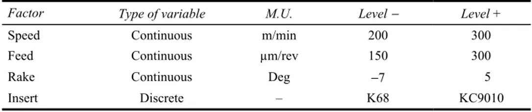
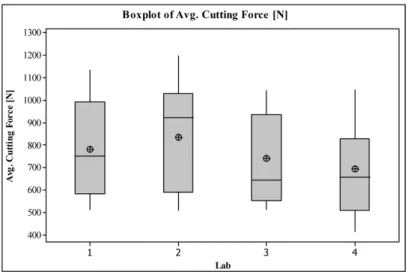
Cutting force is the most critical component of every turning process analysis and optimisation. Particular attention must be paid, from an industrial point of view, because power consumption and cost are strictly related with this component. The overall amount of the data is shown in a boxplot, divided between different laboratories (Figure 1). Figure 1 Boxplot of the cutting force divided for laboratory
The great variability of the data can be noted, as resumed in Table 3. It is clear that such a great variability depends on some specific causes. The quantification of them will be the main goal of ANOVA. Even if they are very significant, standard deviations seem to be very similar. The four medians (rather than the means) are very close, except for Lab2. This overestimation may be influenced by the lack of observations.
Table 3 Collected statistics for cutting force by laboratories
Lab Observed Mean [N] Median [N] Range [N] St. Dev [N] AD test
Lab 1 32 779.90 751.06 622.08 218.47 1.82 Lab 2 28 835.41 923.49 690.30 242.12 1.74 Lab 3 23 742.46 643.54 529.12 195.60 1.37 Lab 4 32 694.33 658.25 631.75 203.43 0.71 The grouped data depart from normality, as confirmed by the Anderson and Darling (AD) test. This test is used to verify if a sample of data comes from a population with a specific distribution. The test makes use of the specific distribution in calculating critical values, thus it appears powerful and attractive (D’Agostino and Stephens, 1986). The goodness-of-fit of the sample can be assessed by looking at the p-value (the test fails if p-value is less then α = 0.05, or AD > 0.752). By stratifying the data in a hierarchical manner, it is possible to delve into the process, by considering those factors perturbed during experiments. Both one-factor-at-time and other grouped stratification have been considered, even if they are not completely shown in this paper. In particular,
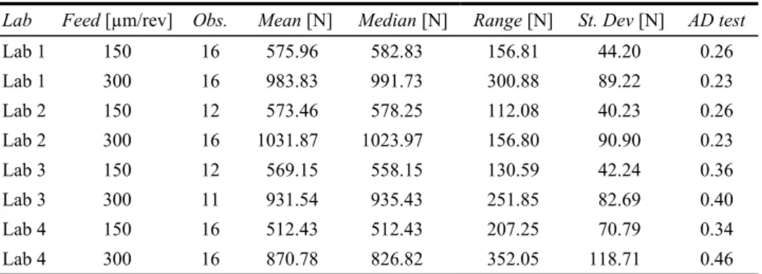
it is interesting to note how the experimental data are correctly represented by a normal distribution, if they are grouped by Feed factor levels. The variation of the Feed factor from the ‘low’ value (150 µm/rev) to the ‘high’ value (300 µm/rev) causes a great increasing of the cutting force. By stratifying the data by Labs and then by Feed, less variability can be noted between the boxes. The interquartile range increases for higher values of Feed and in particular for Lab 4. Greater values of Feed cause an increase of the mean and median values. Table 4 shows the main statistics of the stratified data. Looking at the standard deviations, Lab 4 presents the highest values. AD tests confirm the data are normally distributed (AD < 0.70).
Table 4 Collected statistics for cutting force by laboratories and by feed
Lab Feed [µm/rev] Obs. Mean [N] Median [N] Range [N] St. Dev [N] AD test
Lab 1 150 16 575.96 582.83 156.81 44.20 0.26 Lab 1 300 16 983.83 991.73 300.88 89.22 0.23 Lab 2 150 12 573.46 578.25 112.08 40.23 0.26 Lab 2 300 16 1031.87 1023.97 156.80 90.90 0.23 Lab 3 150 12 569.15 558.15 130.59 42.24 0.36 Lab 3 300 11 931.54 935.43 251.85 82.69 0.40 Lab 4 150 16 512.43 512.43 207.25 70.79 0.34 Lab 4 300 16 870.78 826.82 352.05 118.71 0.46 The boxplot of Figure 2 visualises the data divided into Lab, Feed and then Rake. An appreciable decreasing trend can be noted for every laboratory, when the Rake increases. Lab 4 presents some anomalies, but, generally, no outliers are noted.
3.2 EDA of thrust force
The same analytical approach is implemented for the thrust force. All the same considerations previously achieved for the cutting force component can be maintained for the thrust force. In fact, as the scatterplot (Figure 3) shows, a direct proportionality is evidenced.
Figure 3 Linearity between force components
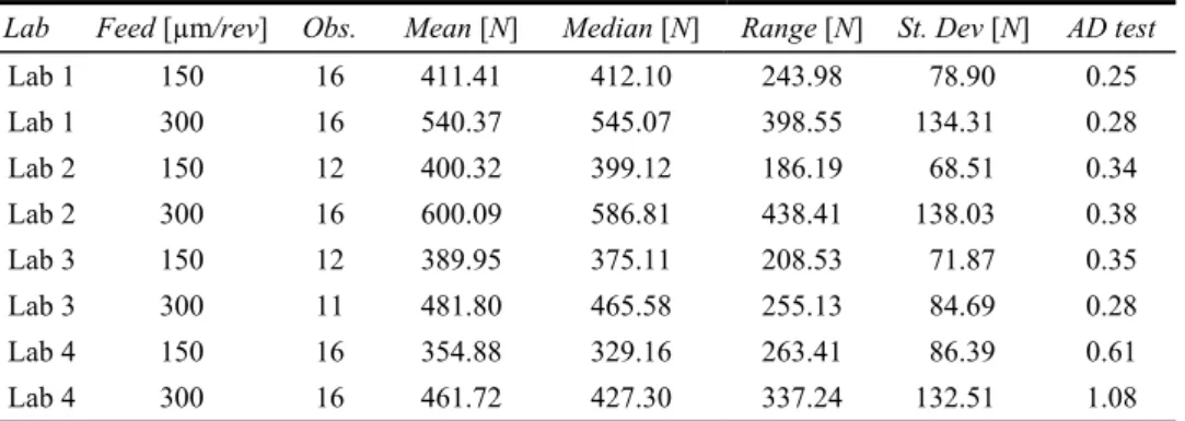
The main statistics of the thrust force are collected, by stratifying the data by different laboratories and, then, by Feed levels (Table 5). AD normality test confirms that the data are approximately normally distributed, except for Lab 4. A consideration can be added: the values measured by Labs 1 and 2, when Feed level is 300 and Rake level –7 are relevantly higher than those of Labs 3 and 4. This discrepancy is highlighted when the Speed factor is set on 200 m/min.
Table 5 Collected statistics for thrust force by laboratories and by feed
Lab Feed [µm/rev] Obs. Mean [N] Median [N] Range [N] St. Dev [N] AD test
Lab 1 150 16 411.41 412.10 243.98 78.90 0.25 Lab 1 300 16 540.37 545.07 398.55 134.31 0.28 Lab 2 150 12 400.32 399.12 186.19 68.51 0.34 Lab 2 300 16 600.09 586.81 438.41 138.03 0.38 Lab 3 150 12 389.95 375.11 208.53 71.87 0.35 Lab 3 300 11 481.80 465.58 255.13 84.69 0.28 Lab 4 150 16 354.88 329.16 263.41 86.39 0.61 Lab 4 300 16 461.72 427.30 337.24 132.51 1.08
4 Analysis of Variance
The EDA showed a lot of unexpected evidence (Mazzola et al., 2007). First of all, four laboratories that operate efficiently obtain quite different results. Therefore, before jumping to some conclusions, it is important to complete the analysis by considering every possible source of variability that could affect the response variables.
The data are structured to define a full-factorial experimental environment. In this case, the ANOVA is the opportune method to quantify the influence of every perturbed factor and of every interaction of them on a specific response variable.
The factors vary between two levels. To obtain a reliable regression, the Laboratory must be considered as a source of variability and, in particular as a noise factor (to be modelled as a block), whose effect should not be relevant. Unfortunately, every laboratory obtained significantly and systematically different results, as shown by the exploratory analyses. For this reason, a full-factorial 24 model with a block fails in representing the real behaviour of the process. In fact, the results of this elaboration demonstrate the effects of factors and interactions, but the model lacks in prediction, because of the erroneous consideration of the Lab variable as a noise (p-values are less than 0.05 for all the blocks and for the lack-of-fit indicator). The combination of machinery and measurement instruments used by different laboratories, in addition to the lack of some observations, affects the variability and influences the adequacy of the model. Thus, a fixed effect ANOVA with five factors, with unbalanced planes is performed, by considering laboratories as a key factor (Ng et al., 1999; Marusich and Ortis, 1995; Montogomery, 1990a; Schmidt and Launsby, 1997). In particular, it is interesting to understand if the difference between laboratories is maintained for every combination of perturbed parameters.
The analysis has been focused on both cutting and thrust force. The objective is to quantify what happens to the force mean and standard deviation values, when the combination of the levels of each factor changes.
4.1 ANOVA of cutting force
For cutting force, a General Linear Model of the ANOVA is performed, by considering Laboratory, Speed, Feed, Rake and Insert factors variable between different levels. Interactions between the five factors are computed up to order three. The first analysis considers the cutting force values and the inferences on the means. The table of the ANOVA (Table 6) shows the combinations of factors and their p-values. P-values less than α = 0.05 means a systematic effect on the response variable. These critical values have been highlighted. One outlier is removed from the data collection (Lab 4, Speed 200, Feed 300, Rake −7 and Insert K68), because the reported value is unreliable.
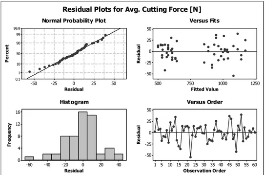
The model is reliable to predict the cutting force values, as confirmed by the correlation index R2, whose adjusted value is 97.5%. In addition, the analysis of the residuals confirms the adequacy of the model (Figure 4).
The coefficients for all the terms included in the model are calculated, demonstrating how the effect of the Feed factor is extremely relevant and causes an average increase of 402 N on the cutting force. Every laboratory affects the overall variability, showing
an insufficient reproducibility of the process (Montgomery, 1990a; Schmidt and Launsby, 1997).
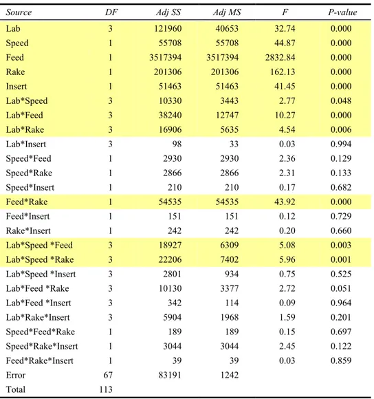
Table 6 ANOVA table: response variable is cutting force (see online version for colours)
Source DF Adj SS Adj MS F P-value
Lab 3 121960 40653 32.74 0.000 Speed 1 55708 55708 44.87 0.000 Feed 1 3517394 3517394 2832.84 0.000 Rake 1 201306 201306 162.13 0.000 Insert 1 51463 51463 41.45 0.000 Lab*Speed 3 10330 3443 2.77 0.048 Lab*Feed 3 38240 12747 10.27 0.000 Lab*Rake 3 16906 5635 4.54 0.006 Lab*Insert 3 98 33 0.03 0.994 Speed*Feed 1 2930 2930 2.36 0.129 Speed*Rake 1 2866 2866 2.31 0.133 Speed*Insert 1 210 210 0.17 0.682 Feed*Rake 1 54535 54535 43.92 0.000 Feed*Insert 1 151 151 0.12 0.729 Rake*Insert 1 242 242 0.20 0.660 Lab*Speed *Feed 3 18927 6309 5.08 0.003 Lab*Speed *Rake 3 22206 7402 5.96 0.001 Lab*Speed *Insert 3 2801 934 0.75 0.525 Lab*Feed *Rake 3 10130 3377 2.72 0.051 Lab*Feed *Insert 3 342 114 0.09 0.964 Lab*Rake*Insert 3 5904 1968 1.59 0.201 Speed*Feed*Rake 1 189 189 0.15 0.697 Speed*Rake*Insert 1 3044 3044 2.45 0.122 Feed*Rake*Insert 1 39 39 0.03 0.859 Error 67 83191 1242 Total 113
In respect to an overall data mean (constant coefficient 755.45 N), Lab 1 and 2 have a similar effect (an average increasing of 24.4 N and 37 N, respectively), but an opposite effect is traced for Lab 3 (−8 N) and, in particular, for Lab 4 (−43.4 N).
Moreover, from an industrial point of view, the significant interactions between Lab*Speed, Lab*Feed and Lab*Rake mean the capability of the laboratories to reproduce the phenomena depends on cutting conditions. The effect of every single factor is visualised on the main effects plot in Figure 5. The dominant effects of Feed and Rake are shown, together with the lower but relevant effects of speed and insert.
Figure 4 Standardised residuals for cutting force
Figure 5 Main effects plot for fitted means of cutting force
Another analysis is performed by looking at the standard deviations of the cutting force, collected for every combination of factors. Each combination has been replicated only twice; thus reliable estimations of standard deviation can be invalidated. It is possible to
try again to consider the variable Lab as a block and to perform a 24 full-factorial design of experiments. In this way, a more feasible experimental field is obtained. Looking at the adequacy of the model, it is possible to assess how a Johnson’s transformation can be useful to represent the data in respect of the normality and omoschedasticity of the residuals (Montgomery, 1990a). The equation (1) represents that the transformation has been applied, where x is the standard deviation value of cutting force.
2.15056 0.667613*ln((+ x+0.108295) / 282.204−x) (1)
Table 7 shows the results of the ANOVA after the transformation and verification of the model adequacy.
In this case, the model is correctly able to represent the process performances. None of the factors perturbed affect the variability; this mean the variability due to the repeatability component is mainly due to natural causes.
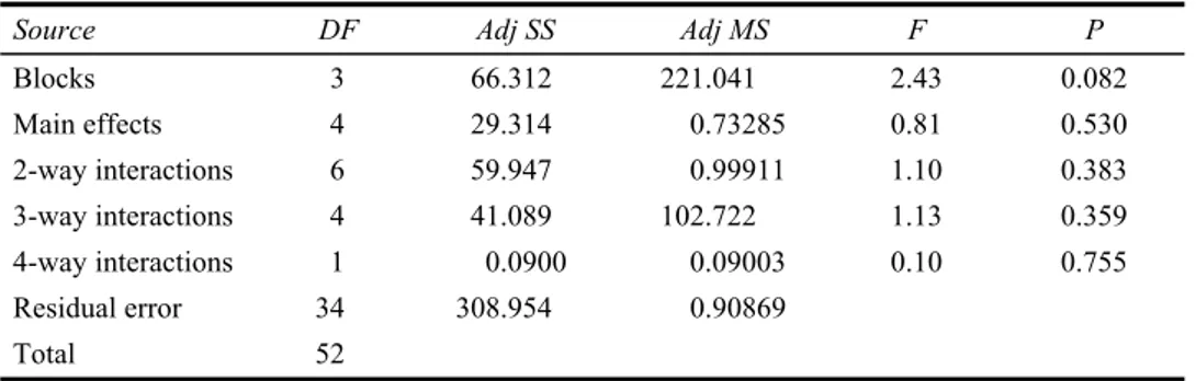
Table 7 Analysis of variance: response is standard deviation of the cutting force
Source DF Adj SS Adj MS F P
Blocks 3 66.312 221.041 2.43 0.082 Main effects 4 29.314 0.73285 0.81 0.530 2-way interactions 6 59.947 0.99911 1.10 0.383 3-way interactions 4 41.089 102.722 1.13 0.359 4-way interactions 1 0.0900 0.09003 0.10 0.755 Residual error 34 308.954 0.90869 Total 52
4.2 ANOVA of thrust force
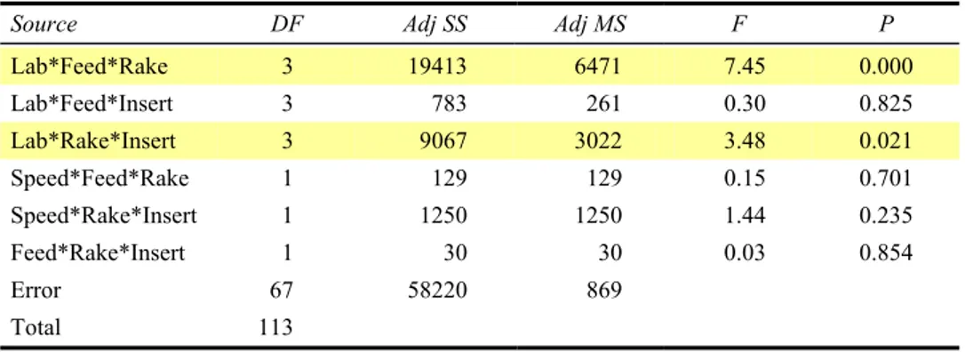
The high correlation between force components is shown on the Scatterplot in Figure 3. The expected influence of factors is proportionally the same noted for cutting force. It is impossible to consider lab variable as a noise factor (this scenario has been tested and the model fails); thus a 25 full-factorial experimental unbalanced design is considered. The ANOVA is performed and the ANOVA table collects the influence of every factor and interaction on the response variable (Table 8). Once again the model correctly represents the process behaviour and the adjusted predictors justify the 94.95% of the overall variability. The interactions are collected up to the third order and the outlier (Lab 4, Speed 200, Feed 300, Rake −7 and Insert K68) is still removed.
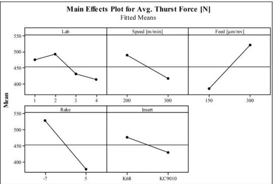
A relevant effect is noted when the Feed is perturbed. An average difference of 137.2 N is estimated when the feed varies between the two levels. The difference between laboratories is appreciable and, in particular, a statistically significant difference is noted for Lab 4. The same laboratory measured four unusual observations, identified as possible outliers, even if their residuals are less than 4R (Montgomery, 1990a). The Rake angle has the greatest weight (when the Rake changes from its low level to the high one an average decreasing of 153.6 N is estimated). For thrust force, the effect of three way interactions become more significant. All the information are visualised on the main effects plot (Figure 6). Once again a complete regression approach is not possible, because the data demonstrate a poor reproducibility of the process.
Figure 6 Main effects plot for fitted means of thrust force
Table 8 ANOVA table: response variable is thrust force (see online version for colours)
Source DF Adj SS Adj MS F P
Lab 3 94660 31553 36.31 0.000 Speed 1 119524 119524 137.55 0.000 Feed 1 408188 408188 469.74 0.000 Rake 1 509662 509662 586.52 0.000 Insert 1 62003 62003 71.35 0.000 Lab*Speed 3 9598 3199 3.68 0.016 Lab*Feed 3 34665 11555 13.30 0.000 Lab*Rake 3 27381 9127 10.50 0.000 Lab*Insert 3 321 107 0.12 0.946 Speed*Feed 1 2822 2822 3.25 0.076 Speed*Rake 1 3750 3750 4.32 0.042 Speed*Insert 1 36 36 0.04 0.840 Feed*Rake 1 60393 60393 69.50 0.000 Feed*Insert 1 5 5 0.01 0.942 Rake*Insert 1 4253 4253 4.89 0.030 Lab*Speed*Feed 3 7884 2628 3.02 0.036 Lab*Speed*Rake 3 20177 6726 7.74 0.000 Lab*Speed*Insert 3 2007 669 0.77 0.515
Table 8 ANOVA table: response variable is thrust force (see online version for colours) (continued)
Source DF Adj SS Adj MS F P
Lab*Feed*Rake 3 19413 6471 7.45 0.000 Lab*Feed*Insert 3 783 261 0.30 0.825 Lab*Rake*Insert 3 9067 3022 3.48 0.021 Speed*Feed*Rake 1 129 129 0.15 0.701 Speed*Rake*Insert 1 1250 1250 1.44 0.235 Feed*Rake*Insert 1 30 30 0.03 0.854 Error 67 58220 869 Total 113 5 Regression approach
From a statistical point of view, the influence of the factor Lab implies the difficulty in finding a general model useful to compare virtual data. Clearly, the validation of some models (the authors particularly refer to simulative models) assesses the respect of proportions and the agreement of trends between real data and virtual ones.
The analyses previously explained can help in understanding a real opportunity: it is necessary to share a common measurement method when the data are collected to increase the reproducibility of the process. The dataset shows good repeatability and the ANOVA could only estimate the components of variability due to the perturbation of some factors.
From an industrial point of view, it is not only interesting to know what is the effect of factors on response variables, but above all to understand the behaviour of response variables through a reliable regression. To assess a reliable regression approach and to evaluate the capability of laboratories to predict the response variables under various perturbations, the data of Laboratory 1 are considered. In this paper, the regression aims to predict the behaviour of cutting force when feed, rake angle, insert type and speed vary.
The data of Lab 1 seem to agree with Kronenberg’s derived expression (2), they do not present outlier and the experimental plane becomes balanced. The theoretical expression for the cutting force (Fc) estimation is
[ ]
* * C x y k F s N f d = (2)where f is the Feed (expressed in mm/rev), d the depth of cut (1 mm), s = f*d for orthogonal cutting and k is the specific strain (N/mm2), function of Rake angle and material type (for AISI 1045, Rm = 680 N/mm2, k = (2962.5 − 20.83*γ) N/mm2). x and y
values depend on the material (for AISI 1045 steel, x = 0.17 and y ≈ 0).
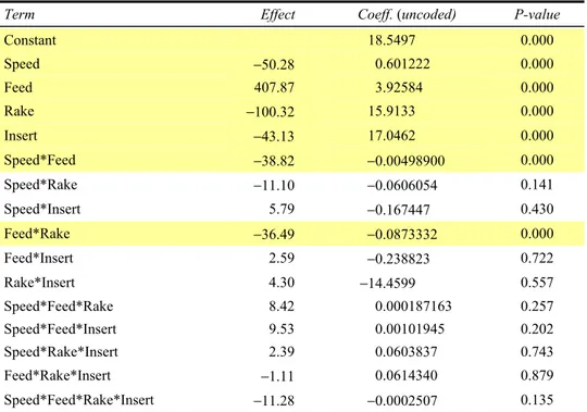
In total, 32 data are considered and the ANOVA is performed. To perform the analysis, the factor Insert is coded (level ‘−1’ means insert type K68 and level ‘+1’ KC9010).
Table 9 Analysis of variance for Lab 1: response variable is cutting force (see online version for colours)
Term Effect Coeff. (uncoded) P-value
Constant 18.5497 0.000 Speed −50.28 0.601222 0.000 Feed 407.87 3.92584 0.000 Rake −100.32 15.9133 0.000 Insert −43.13 17.0462 0.000 Speed*Feed −38.82 −0.00498900 0.000 Speed*Rake −11.10 −0.0606054 0.141 Speed*Insert 5.79 −0.167447 0.430 Feed*Rake −36.49 −0.0873332 0.000 Feed*Insert 2.59 −0.238823 0.722 Rake*Insert 4.30 −14.4599 0.557 Speed*Feed*Rake 8.42 0.000187163 0.257 Speed*Feed*Insert 9.53 0.00101945 0.202 Speed*Rake*Insert 2.39 0.0603837 0.743 Feed*Rake*Insert −1.11 0.0614340 0.879 Speed*Feed*Rake*Insert −11.28 −0.0002507 0.135 A 24 full-factorial experimental plane is considered and the ANOVA is applied to this group of data. The reduced model results adequate to predict the data of Laboratory 1 (the analysis of residuals confirms normality, omoschedasticity and casualty), even if the amount of information becomes quite poor. The adjusted R2 index value is 99.14%. Table 9 collects the effects of every factor and interaction, the coefficients for the regression curve and the relative incidence on the cutting force (looking at the p-values). The estimated coefficients are expressed in uncoded units. The variable Insert can assume only the discrete values ±1.
The main effects are all relevant and the statistical incidences of Feed and Rake agree with the theoretical expression. In addition, the significant effect of Speed, Insert and of Speed*Feed and Feed*Rake interactions can’t be avoided and they concur to the embellishment of the regression equation. All the effects are visualised on the Pareto chart shown in Figure 7.
The regression equation (3) considers all the factors and interactions whose p-values are less than 0.05.
18.55 0.6012*Speed 3.926* Feed 15.913* Rake 17.05* Insert 0.005*Speed * Feed 0.087 * Feed * Rake.
C
F = + + +
+ − − (3)
The curves of Figure 8 show how the regression discretely follows the theoretical expression and furnishes an embellishment, because two factors are added. In particular, the agreement between experimental curve and Kronenberg’s expression is more evident when the speed is lower.
Figure 7 Pareto chart of the standardised effects for cutting force
Figure 8 Regression curves for cutting force
An interesting industrial aspect is to use a regression obtained from real data to assess the capability of simulative models. Once the simulation results have been validated it is possible to refine the experimental architecture by inserting some centre points and to embellish the regression curves as a consequence.
6 Conclusion
The paper presented a structured analysis of a cutting process. The use of both qualitative and quantitative methods and tools highlighted the importance of an analytical procedure from an industrial point of view. The main components of turning force are considered, and through ANOVA, the effects of single or combined factors are computed. The perturbations of the Feed and Rake variables strongly affect the variability of the process. Therefore, the effects of the Speed and Insert type cannot be forgotten, together with the influences due to the interaction between two or three factors.
Some statistically important differences are computed between the four different laboratories involved. Great part of the overall variability is due to the poor reproducibility of the measurements and this altered a global reliable regression approach, useful in case this study is used to compare real data with simulated ones.
Finally, a regression attempt is shown, by considering the data of Laboratory 1. The authors realised a statistical model and relative regression curves, to be considered as an embellishment of a theoretical equation already existing in literature.
Further developments of this work will be the simulation of the data with a dynamic FEM simulator of machining processes, the assessment of software predictability and the addition of some centre points to the experimental architecture to verify and improve the regression curve with an increased sample.
Acknowledgements
The authors wish to acknowledge Mrs. Mary Flynn who checked the manuscript.
References
D’Agostino, R.B. and Stephens, M.A. (1986) Goodness of Fit Techniques, Dekker, New York, NY. Ivester, R.W., Kennedy, M. and Davies, M. (2000) ‘Assessment of machining models: progress report’, Proceeding of the 3rd CIRP International Workshop on Modeling of Machining
Operations, August, Sydney, Australia, pp.511–538.
Ivester, R.W., Kennedy, M. and Davies, M. (2002) ‘Accelerated wear tests for the assessment of machining models calibration data’, Machining Science and Technology, Taylor & Francis, London, UK, Vol. 6, No. 3, pp.487–494.
Ivester. R.W. and Kennedy, M. (2004) ‘Comparison of machining simulations for 1045 steel to experimental measurements’, Society of Mechanical Engineering IMTS Conference 2004, September, Chicago, IL.
Kalpakjian, S. and Schmid, S. (2006) Manufacturing Engineering and Technology, 5th ed., Prentice-Hall, Englewood Cliffs, NJ.
Kronenberg, M. (1966) Machining Science and Application, Pergamon Press, London, UK. Marusich, T.D. and Ortiz, M. (1995) ‘Modelling and simulation of high-speed machining’,
International Journal for Numerical Methods in Engineering, Vol. 38, No. 21, pp.3675–3694.
Mazzola, M., Gentili, E. and Aggogeri, F. (2007) ‘Exploratory data analysis of a turning process’,
Proceeding of the 20th Computer Aided Production Engineering Int. Conference CAPE 2007,
June, Glasgow, UK.
Montgomery, D.C. (1990a) Design and Analysis of Experiments, John Wiley & Sons, New York, NY.
Montgomery, D.C. (1990b) Introduction to Statistical Quality Control, John Wiley & Sons, New York, NY.
Ng, E.G., Aspinwall, D.K., Brazil, D. and Monaghan, J. (1999) ‘Modelling of temperature and forces when orthogonally machining hardened steel’, International Journal of Machine
Tools and Manufacture, Vol. 39, No. 6, pp.885–903.
Özel, T., Hsu, T.K. and Zeren, E. (2005) ‘Effect of cutting edge geometry, workpiece hardness, feed rate and cutting speed on surface roughness and forces in finish turning of hardened AISI H13 steel’, International Journal of Advanced Manufacturing Technology, Vol. 25, No. 3, pp.262–269.
Ranganath, B.J. (1993) Metal Cutting and Tool Design, Vikas, Delhi, India.
Schmidt, S.R. and Launsby, R.G. (1997) Understanding Industrial Designed Experiments, Air Academy Press & Associates, Colorado Springs, CO.
Settineri, L., Zompi, A. and Levi, R. (2005) ‘Numerical and experimental metal cutting analysis: an appraisal’, Proceedings of the 7th Advanced Manufacturing System and Technology