Pierani, P., & Tiezzi, S. (2017). Rational Addiction and Time Consistency: an Empirical Test. In Health Economics Data Group Working paper (pp. 1-22). York : The University of York.
This is the peer reviewd version of the followng article:
Rational Addiction and Time Consistency: an Empirical Test
Publisher:
Terms of use:
Open Access
(Article begins on next page)
The terms and conditions for the reuse of this version of the manuscript are specified in the publishing policy. Works made available under a Creative Commons license can be used according to the terms and conditions of said license. For all terms of use and more information see the publisher's website.
Availability:
The University of York
This version is available http://hdl.handle.net/11365/1005671 since 2017-11-20T11:23:28Z
WP 17/05
Rational Addiction and Time Consistency:
an Empirical Test
Pierpaolo Pierani and Silvia Tiezzi
March 2017
0
RATIONAL ADDICTION AND TIME CONSISTENCY: AN EMPIRICAL TEST
Pierpaolo Pierani^ and Silvia Tiezzi*
This version: March 2017
ABSTRACT
This paper deals with one of the main empirical problems associated with the rational addiction model, namely that the demand equation derived from the rational addiction theory is not empirically distinguishable from models with forward looking behavior, but with time inconsistent preferences. The implication is that, even when forward‐looking behavior is supported by data, the standard rational addiction equation cannot identify time consistency in preferences. In fact, we show that the possibility of testing for exponential versus non‐exponential time discounting is nestled within the general rational addiction model. We propose a test that uses only the information obtained from the general specification and the price effects. We use a panel of Italian individuals to estimate a rational addiction model for tobacco. GMM estimators deal with errors in variables and unobserved heterogeneity. The results conform to the theoretical predictions. We find evidence that tobacco consumers are forward looking. Our test of time consistency does not reject the hypothesis that smokers in our sample actually discount exponentially. JEL codes: C23, D03, D12
Keywords: rational addiction, general versus standard empirical specification, time consistency,
GMM. ^ Department of Economics and Statistics, University of Siena (I), Piazza San Francesco, 7 53100 Siena (I), email: [email protected] * Corresponding author. Department of Economics and Statistics, University of Siena (I), Piazza San Francesco, 7 53100 Siena (I), email: [email protected]
1 1. INTRODUCTION
Becker and Murphy (1988) explored the dynamic behavior of consumption of addictive goods, pointing out that many phenomena previously thought to be irrational are in fact consistent with optimization according to stable preferences. In their model, individuals recognize both the current and future consequences of consuming addictive goods. This model of rational addiction has subsequently become the standard approach to modeling consumption of goods such as cigarettes. A sizable empirical literature has emerged since then, beginning with Becker, Grossman and Murphy (1994), which has tested and generally supported the empirical predictions of the Becker and Murphy model. These past contributions, however, run into a number of critical drawbacks. This paper is concerned with one of these problems, namely that forward‐looking behavior, implied by the model, does not imply time consistent preferences (Gruber and Köszegi, 2001). Indeed even when evidence of forward looking behavior is found, the standard rational addiction demand equation does not allow to separately identify the short‐run and long‐run discount factor applied to future periods consumption (Picone, 2005). This is a crucial issue, because dynamic inconsistency can deliver radically different implications for government policy. In particular, while time consistency implies that the optimal tax on addictive goods should depend only on the externalities imposed on society, time inconsistency suggests a much higher tax depending also on the “internalities” that drugs’ use imposes on consumers themselves (Gruber and Köszegi, 2001). The main contribution of this paper is to show that the possibility of testing for time consistency is nestled within the general rational addiction demand equation. Rather than relying on additional assumptions or on a different theoretical or empirical framework, we use price effects and the general formulation of the rational addiction model to develop a test of time consistency. The purpose is to check whether consumers behind our data reveal time consistent preferences or not. Specifically, this paper offers two distinct empirical contributions to the literature on addiction and time preferences. First, it provides an estimate, using panel data at the individual level, of the general specification of the rational addiction demand equation that includes current, past and future prices1. As far as we know this general specification has been estimated only by Becker,
Grossman and Murphy (1994), Chaloupka (1991), and Waters and Sloan (1995).
1 We use the expression “general specification” of the demand equation as opposed to the most common and well known
“standard specification” which is usually estimated in the empirical literature on rational addiction. While the general specification includes current, past and future prices of the addictive good among the explanatory variables, the standard version only includes current prices. We shall return on this.
2
Second, a simple test of time consistency is developed, which exploits only the information revealed by the general rational addiction demand equation and price effects. Our purpose is to identify between time‐consistent versus time inconsistent agents, and not to identify the exact shape of time discounting.
The implications of our findings are the following. First, the rational addiction model and its derived general demand equation (Becker and Murphy, 1988 and Becker, Grossman and Murphy, 1990) are more general than the previous literature has argued. In particular, they can discriminate between time consistent and time inconsistent consumers. Second, the possibility of distinguishing time consistent from time inconsistent agents is nestled within the same general specification. Stated differently, the information extracted from the general rational addiction demand equation is sufficient to test for both forward‐looking behavior and time consistency. The possibility of testing for time consistency using field data opens up the opportunity of using the rational addiction demand equation to predict the impact of price measures on consumption of addictive goods in a more general way. The remainder of the paper is structured as follows. Section 2 summarizes the literature on time consistency and addiction. Section 3 reviews the general formulation of the rational addiction model used to develop a test of time consistency and introduces our test strategy. Section 4 discusses the data. Section 5 explains the estimation methods and the instruments choice. Results are shown in Section 6. Section 7 concludes. 2. LITERATURE The early literature on dynamic consumption behavior modeled impatience in decision making by assuming that agents discount future streams of utility or profits exponentially over time. Exponential discounting is pivotal. Without this assumption, inter‐temporal marginal rates of substitution will change as time passes, and preferences will be time inconsistent (Strotz, 1956). Recently, behavioral economics has built on the work of Strotz (1956), to explore the consequences of relaxing the standard assumption of exponential discounting. Ainslie (1992) and Loewenstein and Elster (1992) indicate that hyperbolic discounting may explain some basic features of inter‐temporal decision‐making that are inconsistent with simple models of exponential discounting, namely that hyperbolic discounters value consumption in the present more than any delayed consumption. In the formulation of quasi‐hyperbolic discounting adopted by Laibson (1997), for example, the degree of present bias is captured by an extra discount parameter ∈ 0,1) which accounts for instant
3
gratification. Accordingly, the consumption path planned at each time period for the future time periods is never realized, because the inter‐temporal trade‐off changes over time. In Laibson (1997) and Gruber and Köszegi (2001) the decision agent is split into T selves, and they play an intra‐
personal game where one self has to strategically predict the move of his “descendants”. The
decision agent is sophisticated if his predictions about the other selves are correct, naïve otherwise. In either case, the plan made by the first time period self is never fully executed, like the implicit assumption made by the authors.2 In these models present bias can lead individuals to greatly over‐
consume the addictive good, with the consequence of a substantial welfare loss.
The implications of time inconsistent preferences, and their associated problems of self‐control, have been studied under a variety of economic choices and environments. Laibson (1997), O’Donoghue and Rabin (1999a and b) and Angeletos et al. (2001) applied this formulation to consumption and saving behavior. Diamond and Köszegi (1998) explored retirement decisions. Barro (1999) applied it to growth. Gruber and Köszegi (2001), Ciccarelli, Giamboni and Waldmann (2008) and Levy (2010) to smoking behavior. Shapiro (2005) to caloric intake. Fang and Silverman (2009) to welfare program participation and labor supply of single mothers with dependent children. Della Vigna and Paserman (2005) to job search (see Della Vigna 2009 for a review) and Acland and Levy (2010) to gym attendance.
Few works have attempted to use a parametric approach to estimate structural dynamic models with hyperbolic time preferences (Fang and Silverman, 2009; Laibson, Repetto and Tobacman, 2007; Paserman, 2008). Focusing on addictive goods, Levy (2010) derives estimates of the degree of present bias using a model of cigarette addiction based on O’Donoghue and Rabin’s (2002) generalization of Becker and Murphy’s (1988) rational addiction model. Gruber and Köszegi (2001) develop a quasi‐hyperbolic theory conjecturing that individuals are time inconsistent. Under this theory, the individuals would always change their plan and regret their earlier decisions. The authors propose using their model to obtain the present bias and long‐run discounting parameters and, in a previous version of the same paper, they propose a test of time consistency per se. Ciccarelli, Giamboni and Waldmann (2008) tested for time preferences exploring smoking by women before, during and after pregnancy using the European Community Household Panel (ECHP). Their specification does not match the original rational addiction demand equation. They use instead a modified specification with several lead consumption terms, and make inferences about the time preferences of the underlying actors assuming that, if preferences are time consistent, smoking at
4
t+1 is a sufficient statistic for the whole stream of future smoking, i.e., expected smoking more than
one period ahead should have no independent effect on smoking.
To our best knowledge no research has to date tested the assumption of time consistency within the structural demand equation derived from the rational addiction model of Becker and Murphy (1988). As pointed out by Picone (2005), the standard version of the rational addiction demand equation does not allow identification of the short and long run discount factor thus making it impossible to empirically test for time consistency of the agents. In fact, as we shall explain in the next section, the less well known general formulation of the rational addiction demand equation opens the possibility of testing for time consistency.
3. THE GENERAL RATIONAL ADDICTION DEMAND EQUATION AND THE TEST OF TIME CONSISTENCY
Following Becker, Grossman and Murphy (1994, BGM henceforth), we assume a single addictive good C and a composite non‐addictive good Y. Considering time as discrete, the individual maximizes the following utility function:
∑ , , , (1)
Where is the discount factor, and is the rate of time preference assumed to be equal to
the discount rate . et represents unmeasured variables that have an impact on utility at time
t, At is the stock of the addictive good at time t, and the composite commodity Y is taken as the
numeraire. The utility function has the following properties: 0; 0; and 0. This
maximization is subject to the lifetime budget constraint:
∑ ,
Where W0 is the present value of wealth and Pt is the price of the addictive good at time t. The
evolution of the addictive stock At is described by the simple investment function3:
At = Ct‐1 + (1‐)At‐1 (2)
Where is the constant depreciation rate of the addictive stock over time and represents “the
exogenous rate of disappearance of the effects of the physical and mental effects of past consumption” (Becker and Murphy, 1988, p. 677). When the stock depreciates completely in one
5
time period, the depreciation rate is = 1, the depreciation factor becomes (1‐) = 0 and equation (2) becomes: At = Ct‐1. Assuming this restriction holds, considering a quadratic instantaneous utility
function in three arguments Yt, Ct and At subject to the inter‐temporal budget constraint, and solving
the first‐order conditions for Ct and At BGM obtain the following second‐order difference demand
equation: 1 3 2 1 1 1 0 t t t t t t C C P e e C (3) Equation (3) gives current consumption as a function of past and future consumption, the current price Pt and the unobservable shift variables et and et+1. This is the restricted or standard formulation
of the rational addiction demand equation usually estimated in the empirical literature (Baltagi and Griffin 2001 and 2002; Baltagi and Geishecker 2006; Grossman and Chaloupka 1998; Grossman, Chaloupka and Sirtalan 1998; Gruber and Köszegi 2001; Jones and Labeaga 2003; Labeaga 1993 and 1999; Liu et al. 1999; Olekalns and Bardsley 1996; Saffer and Chaloupka 1999, among others). In the more general case, when 1 we have past and future prices entering equation (3) (see BGM, 1990, p. 22; Chaloupka, 1990, p. 11; Picone, 2005, p. 5): 1 1 1 1 (4) Where (Chaloupka, 1990, p. 43):
1 ) 1 ( 1 1 0 uA uC (5) Ω 1 0 (6) 0 (7) 1 1 0 (8) Where the lower case letters denote the coefficients of the quadratic utility function and µ is the marginal utility of wealth. In addition: / /6
Equation (4) is a generalization of equation (3). The future terms in this formulation are discounted at the rate
1
since the future is discounted at the rate and the stock depreciates at the rate (BGM, 1990, p. 24).With quasi‐hyperbolic time preferences, an extra discount parameter ∈ 0,1) capturing instant gratification is added to the model. Therefore, the discount factor between future consecutive periods is γ, but the discount factor between the current and next period is βγ. Equation (4) becomes (Picone, 2005):
1 1 1 1
(4a)
Empirical estimates of equation (4) or (4a) cannot identify γ and β separately. They will instead estimate γβ. This identification problem has so far prevented researchers from empirically testing the hypothesis of time consistency in the rational addiction model. However, time consistent and quasi‐hyperbolic preferences, for example, have radically different policy implications (Gruber and Köszegi, 2001). Because quasi‐hyperbolic individuals tend to over‐consume the addictive good, the optimal value of a Pigouvian tax on addictive goods’ consumption, for example, increases drastically when present biased (instead of time consistent) consumers are considered. This is because the internal costs of impatience add to the external costs caused by consumption of the addictive goods when calculating the optimal level of the Pigouvian tax. For this reason, testing the assumption of time consistency – implied by the rational addiction theory – is of crucial importance to assess the ability of the rational addiction model to give useful policy indications. A serious problem in estimating the general specification (4) is the likely high collinearity between prices, possibly resulting in low statistical significance of the relevant effects. To overcome this problem BGM (1990) impose the restrictions implied by theory. In particular, the restriction that the coefficients Pt+1 and Ct+1 are equal to the past effects multiplied by γ. BGM (1990) and Chaloupka
(1990) find that this restriction is valid and improves the statistical significance of the price and consumption coefficients. The difficult identification of price effects in the general specification explains why the vast empirical literature on rational addiction has focused on estimating the standard equation (3). Indeed, as far as we know, the general specification has been estimated only a few times before. However, its great advantage is that it allows for deeper insights into inter‐ temporal preferences, due to the condition that both the ratio of future‐to‐past consumption coefficients and the ratio of future‐to‐past price coefficients equal the discount factor, . The ratio of future‐to‐current price effects is
7
2 1 1 1 1 t t t t P C P C (9) When the exogenous depreciation is 100% (and (1‐, equation (9) reduces to zero. The ratio of future‐to‐past price effects is, instead ) 1 ( 1 1 1 t t t t P C P C (10) Finally, the ratio of current to past price effects is
1 1 1 2 1 t t t t P C P C (11) When the exogenous depreciation is 100% (and (1‐, the denominator of this ratio is zero. If instead the ratio of future to past consumption effects is considered we have
1 1 1 1 t t t t C C C C (12)To test for time consistency our strategy is to stick to the general specification of the rational addiction demand function, arguing that information obtained by the estimation of this equation is sufficient. To test whether data support exponential discounting, we exploit price effects from equation (4) and compare the discount factor obtained from equation (11):
, (13)
with the discount factor obtained from equation (9):
, (14)
In (13) α , α , α are parameters of the empirical model (15) to be estimated, and the discount factor is obtained comparing price effects at time t and t‐1, in equation (14) it is instead obtained comparing price effects at time t+1 and t. Under the null hypothesis of time consistency, and conditional on a given depreciation rate, the two ratios are equal at a given significance level. Our test thus consists of testing the null hypothesis that the two ratios (13) and (14) are statistically the same.
8 4. DATA
The most appropriate form of data to capture the key features of these dynamic models with unobserved heterogeneity is individual level panel data. Unfortunately, panel data at the individual level to test this type of models do not exist in Italy. To implement our test we have built a pseudo panel using monthly cross sections from January 1999 to December 2006 of individual Italian household current expenditures on tobacco products (cigarettes, cigars, snuff tobacco and cut tobacco) collected by Istituto Nazionale di Statistica (ISTAT) through a specific and routinely repeated survey called “Indagine sui Consumi delle Famiglie”4. ISTAT uses a weekly diary to collect
data on frequently purchased items and a face‐to‐face interview to collect data on large and durable expenditure. Two weeks in each month are randomly selected and households sampled in each month are divided in two groups of equal number and assigned to one of the two randomly selected weeks. Current expenditures are classified in about 200 elementary goods and services with the exact number changing from year to year due to minor adjustments in the item’s list. The survey also includes detailed information on the household structure, and socio‐demographic characteristics (such as regional location, number, gender, age, education and employment condition of each household member). All annual samples are independently drawn according to a two‐stage design5. Monthly and regional consumer price indices (1998=100) for tobacco matching
expenditures reported in the “Indagine sui Consumi delle Famiglie” are also available from ISTAT. Given the above survey design, it is impossible to track individual households over time and, therefore, to estimate a DPD model. To overcome this problem, we start from the series of independent cross‐sections of micro‐data for the period 1999(1)‐2006(12) and we construct a pseudo panel using cell averages to identify household. Households in each cell are selected based on 12 combinations of available demographic characteristics plus one residual category, and sample averages for each type in each month and in each region have been computed. Since the survey does not provide information on the number of tobacco consumers in the household, households with one member only are selected to avoid any ambiguity between the recorded expenditure and the individual in the household. Eventually, data have been organized as a pseudo panel Φ(r, f, m, t), by stacking up monthly data (m =1, …, 12) for each year (t = 1, …, 8) and for each macro region (r 4 A different sample of households is interviewed each month; the items list also includes semi‐durable expenditures, with a total number of about 280 goods and services.
5 Details on the sampling procedure used to collect these data can be found in ISTAT, Indagine sui Consumi delle
9 = 1, …,4) on each household type (f = 1, …,13) in vectors whose length varies each period. The final dataset is an unbalanced panel of 4,259 mean single households observations. Our dependent variable, the quantity of tobacco consumed, has been obtained implicitly as the ratio between monthly tobacco expenditure (in Euros) and the tobacco price index. In order to introduce some individual variation, the price of tobacco is constructed by deflating the retail price index for tobacco by a weighted average of nine broad categories of the retail price index, as in Labeaga (1999), where the weights are the shares of expenditure devoted to each good in each household. A set of dummy variables is included to account for socio‐demographic and geographic factors: location: northwest (NW), northeast (NE), center (CE), south and islands (SI); gender; employment status (employed, unemployed); education level (higher education, lower education); income level (rich, poor, middle); age (less than 24 years; between 25 and 65 years and more than 65 years); household type (1 to 13). We also add total current monthly expenditure as a proxy of disposable income. Summary statistics of the data are shown in Table 1. Almost 22% of single households report zero tobacco expenditures during the survey period. On average, tobacco consuming singles have slightly higher total expenditures than non‐consuming ones. Non‐consuming females are more numerous than non‐consuming males. When looking at age, young consumers are less represented than older ones in our data, but among non‐consuming households the young are more numerous than the old. There are also more highly educated non‐consumers than less educated non‐ consumers and more unemployed non‐consumers than employed non‐consumers.
Table 1 - The Data
Variable Full Sample Consuming
Household Non-consuming Household Sample size 4,259 3,304 955 Tobacco expenditurea 14.044 (16.390)b 18.104 (6.516) 0 Price of Tobacco 113.161 (9.911) 113.115 (9.857) 113.319 (10.096)
Retail price index 110.527
(5.905) 110.635 (5.856) 110.153 (6.060) Total expenditure 1414.426 (544.657) 1420.022 (504.472) 1395.066 (665.167)
Dummy variables (yes = 1, no = 0)
Northwest 0.255 (0.436) 0.268 (0.443) 0.212 (0.409) Northeast 0.2444 0.241 0.258
10 (0.429) (0.427) (0.437) Centre 0.241 (0.428) 0.234 (0.423) 0.268 (0.443)
South & Islands 0.259
(0.438) 0.258 (0.438) 0.268 (0.439) Male 0.449 (0.497) 0.469 (0.499) 0.381 (0.485) Female 0.469 (0.499) 0.459 (0.498) 0.504 (0.500) Unemployed 0.312 (0.464) 0.246 (0.431) 0.541 (0.498) Employed 0.359 (0.479) 0.422 (0.494) 0.139 (0.346) Young (< 24) 0.067 (0.250) 0.042 (0.201) 0.154 (0.361) Adult 0.671 (0.469) 0.669 (0.471) 0.681 (0.466) Senior (>65) 0.180 (0.384) 0.218 (0.413) 0.050 (0.218) Low Education 0.355 (0.478) 0.366 (0.482) 0.315 (0.465) High Education 0.317 (0.465) 0.303 (0.459) 0.365 (0.482) Low income 0.249 (0.433) 0.231 (0.421) 0.315 (0.465) High income 0.249 (0.433) 0.249 (0.432) 0.252 (0.435) Notes:
a Monthly expenditures in Euros b Standard deviations in parentheses.
Source: ISTAT, “I Consumi delle Famiglie”, years 1999-2006.
5. ESTIMATING THE GENERAL RATIONAL ADDICTION MODEL Our empirical demand equation is a variant of equation (4): it t i it it it it it it it C C P P P X v d u C 01 12 13 4 15 16 (15)
whereCitis tobacco consumption of individual i in period t,Pitis tobacco price,Xitis a vector of
exogenous economic and socio‐demographic variables that affect consumption of tobacco,viare
individual fixed effects capturing time invariant preferences that are correlated with lead and lagged consumption and probably with other determinants of consumption,dtare time fixed effects, and 1 3 2 t t it e e u is the idiosyncratic error term. There are two problems that will bias OLS estimates of the dynamic panel data equation (15). First, there is an omitted variable bias due to unaccounted demand shifters that may also be serially
11 correlated (BGM, 1994). Second, we need to deal with the problem of errors‐in‐variables. In the context of household surveys, consumption data could be subject to censoring, yet in this work we assume that zeroes are attributable to infrequency of purchase only and that the purchase policy is time‐invariant6. Under infrequency of purchase, none of the variables are censored but they are measured with errors7 and are correlated with the mixed error term. To illustrate this problem, suppose we wish to estimate the demand equation (15), but instead of observing the true seriesCit*we observeCit Citmit * , wheremitis the measurement error. Thus the disturbance in the empirical model using the observed data is 1 2 1 1 1 3 2 it it it it it it e e m m m u (16) The error term uitin (16) is serially correlated. Measurement errors lead to the classical error‐in‐
variables model (CEV), which causes an attenuation bias in the estimated coefficients and this problem is worsened using panel data. To correct for this endogeneity bias we follow Arellano and Bond (1991) in using a GMM procedure to obtain the vector of parameters. The GMM estimators exploit a set of moment conditions between instrumental variables and time‐ varying disturbances. The basic idea is to take first‐differences to deal with the unobserved fixed effects and then use the suitably lagged levels of the endogenous and predetermined variables as instruments for the first‐differenced series, under the assumption that the error term in levels is spherical and taking into account the serial correlation induced by the first‐difference transformation. This idea extends to the case of lags and leads of the dependent variable and where serial correlation already exists in the error term of the original model, as in equation (15). After first‐differencing equation (15): it t it it it it it it it C C P P P X d u C 1 1 2 1 3 4 1 5 1 6 7 (17) the strategy is to find a set if instrumentsZitthat are uncorrelated with the first‐differenced error term and correlated with the regressors. By definition uit 1 2 1 1 1 3 2 uit eit eit mit mit mit (18)
6 In the survey on households’ expenditures, data on current consumption purchases are collected for each sampled
household during one week only (within a month). These weekly expenditures are then aggregated to the month by ISTAT using a statistical model accounting for the frequency of purchase of each item, i.e. for the proportion of households purchasing that specific item during the surveyed week. Thus it may well be that a specific household does not purchase tobacco during the surveyed week and its monthly expenditure on that good is set to zero, but this does not imply that her expenditure has been zero in the other three weeks too. Consistent with the hypothesis of infrequency of purchase and time invariant purchase policy, it can be that the frequency of the survey does not coincide with the frequency of purchase.
12
for i1,...,Nand t3,...,T 1. Recalling the error term uitin (16), the following moment
conditions are available 0
) (Citsuit
E for t4,...,T 1ands3
This allows the use of lagged levels of observed consumption series dated t3and earlier as instruments for the first‐differenced equation (17). The moment restrictions can be written in matrix form as ( ' )0
i i u
Z
E for t = 4, …, T ‐ 1, where is the (T‐4) vector ui
' 1 5 4, ,..., ui ui uiT . 1
ui uit uit and Ziis a
T 4
gblock diagonal matrix, whose ith block is given as ' 1 ' 5 ' 4 4 1 2 1 1 : ... ... 0 0 0 : : : ... : : : 0 ... 0 ... 0 0 ... 0 ... 0 0 iT i i iT i i i i i W W W C C C C C Z (19) where the block diagonal structure at each time period exploits all of the instruments available, concatenated to one‐column first differenced exogenous regressorsWit
Pit,Pit1,Pit1,Xit
' that act as instruments for themselves8 (Arellano and Bond, 1991). Ever since the work of BGM (1994) on US cigarette consumption, past and future prices have been considered natural instruments for lagged and lead consumption, as well. In fact, the exclusion of future prices from the their instrument set yields puzzling results, such as wrong signs on interest rate, lagged consumption and own price. So, despite future prices failing a Hausman test, BGM (1994) consider them as valid instruments. We maintain this pivotal option here. Given that price variation over the study period is very limited we argue that agents are able to anticipate tobacco price a month or more from the date of the survey.However, the first‐differenced GMM estimator is poorly behaved in terms of finite sample properties (bias and imprecision) when instruments are weak. This can occur here given that the lagged levels of consumption are usually only weakly correlated with subsequent first‐differences. More plausible results and better finite sample properties can be obtained using a system‐GMM estimator (Arellano and Bover, 1995; Blundell and Bond, 1998). This augmented version exploits additional moment conditions, which are valid under mean stationarity of the initial condition. This assumption yields (T‐4) further linear moment conditions which allow the use of equations in levels with suitably lagged first‐differences of the series as instruments
8 The existence ever since 1862 of a public monopoly for tobacco in Italy justifies our choice of considering tobacco
13
0 ) (Cit2uit
E for t4,...,T 1 (20)
The complete system of moment conditions available can be expressed as ( ' )0
i i u Z E , where
' 1 4 1 4,..., , ,..., iT i iT i i u u u u u . The instrument matrix for this system is given as 3 3 2 ... 0 0 0 . ... . . . 0 ... 0 0 0 ... 0 0 0 ... 0 0 iT i i i i C C C Z Z (21) Whether we actually need all these moment conditions is debatable, since in finite samples there is a bias/efficiency trade‐off (Biørn and Klette, 1998). A large instruments collection, like that generated by system GMM, overfits endogenous explanatory variables and weakens the power of the overidentification tests (Roodman, 2009). Ziliak (1997) showed that GMM may perform better with suboptimal instruments and argued against using all available moments, especially when T is large relative to N. Since in our case N = 52 and T = 96 (hence a large number of orthogonality conditions), we use only a subset of them, testing their validity with the Sargan over‐identification test (Baltagi and Griffin, 2001).After some experimentation, we report estimates using the following parsimonious matrix of instrumentsZi, which represents a compromise between theory and previous applied work, the characteristics of the data and computational limitations9 4 2 1 ' 1 ' 5 5 6 4 2 ' 4 4 5 3 1 , , , ... 0 0 : : ... : : 0 ... , , , 0 0 ... 0 , , , iT iT iT iT iT i i i i i i i i i i i W Y P P C W Y P P C W Y P P C Z (22) Where the proxy of disposable income is also used as an instrument and the least informative lagged levels of consumption have been dropped.10 6. RESULTS The empirical specification of model (15) uses the quantity of tobacco consumed per month as the dependent variable. The right‐hand side variables are the lead and lag consumption, the current
9 The time series dimension in the empirical estimation is T=24 due to computational limitations.
10 Estimation of the model employs a modified TSP program written by Yoshitsugu Kitazawa (2003). The set of TSP
14
lead and lag real price of tobacco, the proxy of disposable income and the following socio‐ demographic characteristics: gender, age, high education, high income and the interactions between price and demographic characteristics. We use a subset of all available instruments of prices. Our chosen estimator is the system–GMM (Blundell and Bond, 1998). This unifying GMM framework incorporates orthogonality conditions of both types of equations, transformed and in levels and performs significantly better in terms of efficiency as compared to other IV estimators of dynamic panel data models. We estimate both one‐step and two‐step system‐GMM estimators, but we only report two‐step estimates with a robust covariance matrix11.
In terms of empirical studies and finite sample properties of the GMM estimator, the choice of transformation used to remove individual effects is of great concern. First differencing (FD) is just one of the many ways. Arellano and Bover (1995) present an alternative transformation for models with predetermined instruments, forward orthogonal deviations (FOD). This transformation involves subtracting the mean of all future observations for each individual. The key difference between FD and FOD is that the latter does not introduce a moving average process in the disturbance, i.e., it preserves orthogonality among errors. Hayakawa (2009) compares the performances of the GMM estimators of dynamic panel data model wherein different transformations are used. His simulation results show that overall the FOD model outperforms the FD model in many cases. Since we have an unbalanced panel, another practical difference is that the FOD transformation preserves the sample size in panels with gaps, where FD would reduce the number of observations12.
Results under the infrequency of purchase interpretation of zeros and three alternative transformation methods are reported in Table 2. The fixed‐effects transformation or within transformation (WT) is reported for the sake of comparison and completeness. For the reasons discussed above, our preferred specification is the system GMM with FOD. On the whole, our estimates are consistent with the rational addiction framework. First, past consumption has a significant positive effect. Second, future consumption has a significant positive effect, supporting the idea that behavior is forward looking. Third, the coefficient of lag consumption is always greater than the coefficient of lead consumption, giving rise to a positive discount rate. Fourth, we obtain a negative coefficient on current price and a positive coefficient on both past and future prices. So, the signs on the two consumption variables and the three price variables conform to theoretical
11 We report two-step estimates even though we are aware that in finite samples a downward bias of the estimated standard
error of the two-step GMM estimator may arise (Davidson and MacKinnon, 2004; Baltagi, 2005).
15
predictions. As to the demographic variables in our specification, being an adult has a positive and significant effect as well as being a high‐income household. A price increase has a positive and significant effect on consumption for single males and for singles with higher education, whereas it has a negative and significant effect for employed singles.
Table 2 – Estimates of General Rational Addiction Models (infrequency or misreporting)
Parameter Gmm_Sys Gmm_Sys Gmm_Sys
WT FOD FD Ct-1 0.506 (0.007) (0.009) 0.483 (0.021) 0.055 Ct+1 0.486 (0.006) 0.461 (0.008) 0.045 (0.020) Pt -0.474 (0.090) (0.093) -0.385 (0.092) -0.515 Pt-1 0.243 (0.042) (0.055) 0.225 (0.052) 0.314 Pt+1 0.229 (0.050) 0.150 (0.057) 0.194 (0.078) Northwest 1.926 (5.020) (3.311) -3.837 Northeast 15.290 (4.979) -14.043 (3.390) Centre 3.373 (4.945) -11.337 (3.126) Male -6.457 (7.303) (4.261) 0.952 (1.266) 6.494 Employed -9.418 (10.427) (6.435) -2.483 (2.295) 1.801 Adult -14.524 (6.427) 11.834 (4.006) 2.790 (1.858) College 12.253 (12.746) (6.507) 1.081 (1.872) -4.993 Rich 3.349 (0.589) (1.160) 2.587 Price*Male 0.014 (0.018) (0.010) 0.041 Price*Employed -0.010 (0.022) -0.038 (0.013) Price*Adult -0.019 (0.023) (0.011) -0.014 Price*College 0.008 (0.068) (0.010) 0.028 Male*Employed 9.987 (20.374) 5.046 (11.400) Male*Adult 0.677 (18.451) -8.497 (10.227) Male*College 4.688 (16.956) -5.644 (9.516)
p-value Sargan test 0.427 0.519 0.322
Consistent standard errors robust to heteroscedasticity are in parentheses.
16 6.1 Dynamics of Consumption Our demand equation is a second‐order difference equation in current consumption. The roots of this difference equation are useful for describing the dynamics of consumption and are positive if and only if consumption is addictive. For equation (3) and (4) these roots are (BGM, 1994 p. 413 or BGM, 1990, p. 9): 2 ) 4 1 ( 1 2 1/2 1 2 ) 4 1 ( 1 2 1/2 2
with 42 1 by concavity. BGM note that both roots are real and depend on the sign of . Both roots are positive if and only if consumption is addictive ( > 0); both roots will be zero or negative otherwise. The smaller root, 1, gives the change in current consumption resulting from a shock to
future consumption. The inverse of the larger root,2, indicates the impact of a shock to past consumption on current consumption. These shocks may be the result of a change in any of the factors affecting demand for cigarettes. Besides the restrictions on the values of the two roots, the conditions necessary for stability include that the sum of the coefficients on past and future consumption is less than unity and that the sum of the coefficients on prices is negative (see Chaloupka, 1990, p. 22). Our results fulfill the stability condition13 as both roots are positive: (λ
2)‐1 =
3.115 (0.052), and λ1 = 0.162 (0.000), and 4 1 (BGM, 1994). Finally, the sum of coefficients on
past and future consumption is less than unity and the sum of price coefficients is negative, as required by theory14.
6.2 Test of Time Consistency
In Table 3 we present the parameters derived from the estimated equation and used for our proposed test of time consistency. These parameters refer to our preferred specification: system GMM with FOD (column 2 of Table 2). The first row shows the discount factor implied by the ratio of the future‐to‐current price coefficients (equation 14). The second row shows the discount factor implied by the ratio of the current‐to‐past price coefficients (equation 13).
13 Baltagi (2007) stresses that, in fact, this is somehow improperly known as a stability condition, because the
solution to a rational addiction model is generally assumed to be a saddle point and its roots could therefore not pass a stability test.
14 In a recent essay Laporte et al. (2017) investigate whether the unstable root ( ) complicates the estimation of the
rational addiction model even when the true data generating process possesses the true characteristics of rational addiction. In our case, however, all the theoretical restrictions implied by theory are satisfied by the data (including a plausible estimate of the discount factor, computed as the ratio of the Ct+1 and Ct-1 coefficients in the second column of Table 2).
17
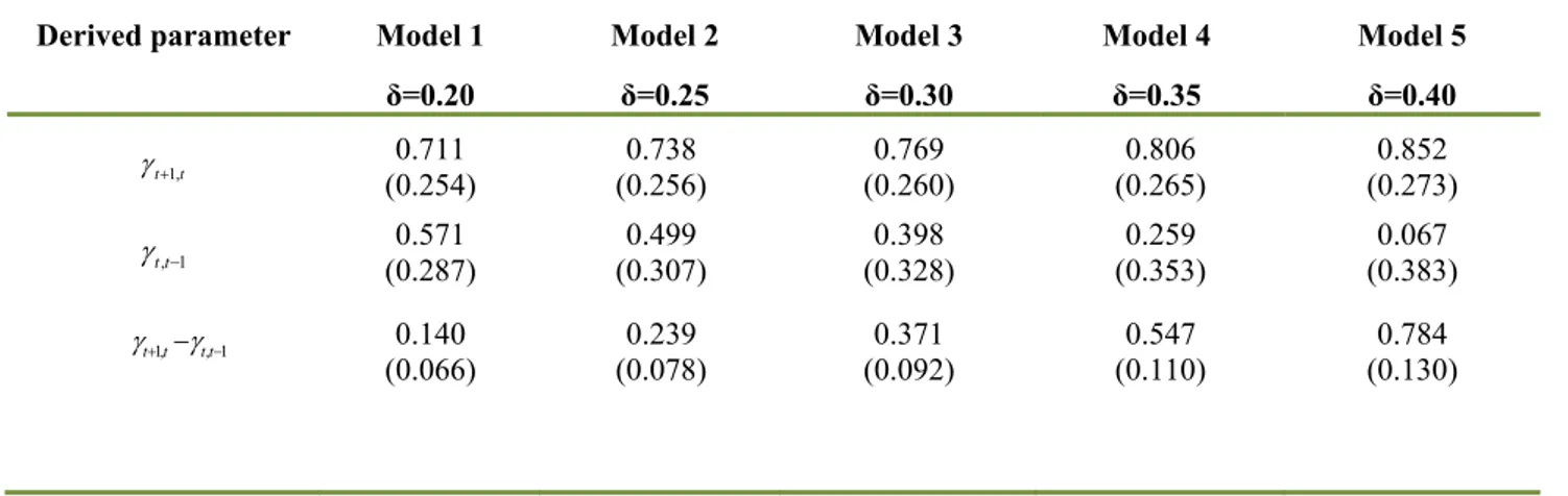
Table 3 – Discount Factors and Time Consistency
Derived parameter Model 1 Model 2 Model 3 Model 4 Model 5
δ=0.20 δ=0.25 δ=0.30 δ=0.35 δ=0.40 t t1, 0.711 (0.254) (0.256) 0.738 (0.260) 0.769 (0.265) 0.806 (0.273) 0.852 1 ,t t 0.571 (0.287) (0.307) 0.499 (0.328) 0.398 (0.353) 0.259 (0.383) 0.067 t1,tt,t1 0.140 (0.066) (0.078) 0.239 (0.092) 0.371 (0.110) 0.547 (0.130) 0.784
Consistent standard errors robust to heteroscedasticity are in parentheses.
We perform the test for five different values of the exogenously set depreciation rate, δ, corresponding to the five columns of results in Table 3. The null hypothesis of time consistency is that the difference between two discount factors is statistically not different from zero. In the third row, for all the selected δ we reject the null hypothesis that the difference is zero, at any level of significance. Focusing on this result only would lead us to conclude that consumers behind our data do not discount exponentially. However, inspection of the first and second row reveals that the confidence intervals of the two discount factors overlap considerably. Because of these mixed results, it is difficult to completely reject the hypothesis that the two estimated discount factors are the same in the estimated models. In case non‐exponential discounting is detected in the data, the proposed test does not allow to further investigate the exact shape of time discounting detected. Suppose the test rejects the null of time consistency. Even hypothesizing quasi‐hyperbolic discount for example, it is not possible to separately identify the short and long‐run discount parameters. Despite these limitations, our findings open up a number of interesting avenues for future research. First, conditional on finding time inconsistency, future efforts should be directed at trying to identify the exact shape of time discounting. Second, the role of the exogenous rate of depreciation δ should be further investigated. Finally, an alternative dataset and a richer specification of the general rational addiction model, including several lags and leads of price and consumption, might produce even better estimates of the parameters.
18 7. CONCLUDING REMARKS
This paper addresses one of the main theoretical and empirical shortcomings of the rational addiction model, namely that forward‐looking behavior, implied by theory, does not necessarily imply time consistency. Then, even when forward looking behavior is supported by data, the dynamic consumption equation derived from the rational addiction theory does not provide evidence in favor of time consistent preferences against a model with dynamic inconsistency (Gruber and Köszegi, 2001).
We show that, in fact, the possibility of testing for time consistency is nestled within the rational addiction demand equation. Rather than relying on additional assumptions or on a different theoretical or empirical framework, we use price effects and the rarely estimated general formulation of the rational addiction demand equation to develop a test of time consistency. The test’s purpose is to check whether consumers behind our data reveal time consistent preferences or not. However, conditional on finding time inconsistency, this test cannot identify the exact shape of time discounting.
Our estimates of the general rational addiction model conform to theory. Our test of time consistency does not completely reject the hypothesis that consumers behind our data actually discount exponentially.
The value added of our contribution is to show that the possibility of distinguishing time consistent from time inconsistent preferences is nestled within the rational addiction model. The information extracted from a general rational addiction demand equation is sufficient to test for both forward‐ looking behavior and time consistency. Future efforts could strengthen these results using alternative transformations of the data and alternative specifications of the general model, trying to identify the exact shape of time discounting in case of detected time inconsistency, and further investigating the role of the exogenous rate of depreciation δ.
19 References Acland, D. and M. Levy (2010) “Habit Formation, Naiveté, and Projection Bias in Gym Attendance.” Working Paper, Harvard University. Ainslie, G. (1992) “Picoeconomics: the Strategic Interaction of Successive Motivational States Within the Person.” Cambridge, UK; New York: Cambridge University Press, 1992.
Angeletos, G., D. Laibson, A. Repetto, J. Tobacman and S. Weinberg (2001) “The Hyperbolic Consumption Model: Calibration, Simulation and Empirical Evaluation.” The Journal of Economic Perspectives, Summer 2001, 15(3), pp. 47‐68. Arellano, M. and O. Bover (1995) “Another look at the Instrumental Variable Estimation of error‐ component Models.” Journal of Econometrics, 68, pp. 29‐51. Arellano, M. and S. Bond (1991) “Some tests of specification for panel data: Monte Carlo evidence and an application to employment equations.” Review of Economic Studies, 58, pp. 277‐297. Baltagi, B. (2005) Econometric Analysis of Panel Data. John Wiley & Sons. Baltagi, B. (2007) “On the use of Panel Data to estimate Rational Addiction Models.” Scottish Journal of Political Economy, 54(1), pp. 1–18.
Baltagi, B.H. and Geishecker, I. (2006) “Rational alcohol addiction: Evidence from the Russian Longitudinal Monitoring Survey.” Health Economics.
Baltagi, B.H. and Griffin, J.M. (2001) “The Econometrics of Rational Addiction: the Case of Cigarettes.” Journal of Business and Economic Statistics, 11: 4, pp. 449‐454.
Baltagi, B.H. and Griffin, J.M. (2002) “Rational addiction to alcohol: Panel data analysis of liquor consumption.” Health Economics, 11, pp. 485‐491.
Barro, R. J. (1999) “Ramsey meets Laibson in the neoclassical growth model.” Quarterly Journal of Economics, 114, pp. 1125‐1152.
Becker, G. S. and K. Murphy (1988) “A Theory of Rational Addiction.” Journal of Political Economy, 96, pp. 675‐701.
Becker, G., M. Grossman and K. Murphy (1990) “An Empirical Analysis of Cigarette Addiction.” Working Paper n. 61‐1990. Centre for the Study of the Economy and the State, University of Chicago. Becker, G. S., M. Grossman, K.M. Murphy (1994) “An Empirical Analysis of Cigarette Addiction.” The American Economic Review, pp. 396‐418.
20
Biørn, E. and T.J. Klette (1998) “Panel data with errors‐in‐variables: essential and redundant orthogonality conditions in GMM‐estimation.” Economics Letters, 59, 3, pp. 275‐282.
Blundell, R. and S. Bond (1998) “Initial conditions and moment restrictions in dynamic panel data models.” Journal of Econometrics, 87, pp. 115‐143.
Chaloupka, F. (1990) “Rational Addictive Behaviour and Cigarette Smoking.” NBER Working Paper n. 3268/1990.
Chaloupka, F. (1991) “Rational Addictive Behavior and Cigarette Smoking.” Journal of Political Economy, 99, 4, pp. 722‐742. Ciccarelli, C., L. Giamboni and R. Waldmann (2008) “Cigarette Smoking, Pregnancy, Forward Looking Behavior and Dynamic Inconsistency”. Munich Personal RePEc Archive N. 8878. Davidson, R. and J.G. Mackinnon (2004) Econometric Theory and Methods. Oxford University Press, 2004. Della Vigna, S. (2009) “Psychology and Economics: Evidence from the Field.” Journal of Economic Literature, August 2009, 47(2), pp. 315‐372. Della Vigna, S. and D. Paserman (2005) “Job Search and Impatience.” Journal of Labor Economics, 23(3), pp. 527‐588. Diamond, P. and B. Köszegi (1998) “Hyperbolic Discounting and Retirement.” Mimeo, 1998. Fang, H. and D. Silverman (2009) “Time‐Inconsistency and Welfare Program Participation. Evidence from the NLSY.” International Economic Review, vol. 50, n. 4, pp. 1043‐1076.
Grossman, M. and Chaloupka, F. (1998) “The demand for cocaine by young adults: A rational addiction approach.” Journal of Health Economics, 17, pp. 427‐474.
Grossman, M., Chaloupka, F. and Sirtalan, I. (1998) “An empirical analysis of alcohol addiction: Results from monitoring the future panels.” Economic Inquiry, 36, pp. 39‐48.
Gruber, J. and B. Köszegi (2000) “Is Addiction Rational? Theory and Evidence.” NBER Working Paper 7507.
Gruber, J. and B. Köszegi (2001) “Is Addiction Rational? Theory and Evidence.” Quarterly Journal of Economics, CXVI, pp. 1261-1303.
Hayakawa K. (2009) “First Difference or Forward Orthogonal Deviation – Which Transformation Should Be Used in Dynamic Panel Data? : A Simulation Study.” Economics Bulletin, Vol. 29,no. 3, pp. 2008‐2017.
Jones, A. and J.M. Labeaga (2003) “Individual Heterogeneity and Censoring in Panel data Estimates of Tobacco Expenditure.” Journal of Applied Econometrics, 18, pp. 157‐177.
21
Labeaga, J.M. (1993) “Individual behaviour and tobacco consumption: A panel data approach. “ Health Economics, 2, pp. 103‐112. Labeaga, J. M. (1999) “A Double‐Hurdle rational addiction model with heterogeneity: estimating the demand for tobacco.” Journal of Econometrics, 93:1, pp. 49‐72. Laibson, D. (1997) “Golden Eggs and Hyperbolic Discounting”. Quarterly Journal of Economics, 62:2, pp. 443‐478. Laibson, D., A. Repetto and J. Tobacman (2007) “Estimating Discount Functions with Consumption Choices Over the Lifecycle.” Working Paper, Harvard University. Laporte, A. , A. Rohit Dass and B.S. Ferguson (2017) “Is the Rational Addiction Model inherently impossible to estimate” Journal of Health Economics. http://dx.doi.org/10.1016/j.jhealeco.2016.12.005 Levy, M. (2010) “An Empirical Analysis of Biases in Cigarette Addiction.” Working Paper, Harvard University. Liu, J‐L., Liu, J‐T., Hammit, J.K., and Chou, S‐Y. (1999) “The price elasticity of opium in Taiwan, 1914‐ 1942.” Journal of Health Economics, 18, pp. 795‐810. Loewenstein, G. and J. Elster (1992) “Choice over Time.” Russell Sage: New York, 1992. O’Donoghue, T. and M. Rabin (1999a) “Doing it Now or Later.” The American Economic Review, 89(1), pp. 103‐124. O’Donoghue, T. and M. Rabin (1999b) “Addiction and Self‐Control.” In Jon Elster, editor, Addiction: Entries and Exits, New York: Russell Sage.
O’Donoghue, T. and M. Rabin (2002) “Addiction and Present Biased Preferences.” University of California at Berkeley, Working paper 1039.
Olekalns, N. and Bardsley, P. (1996) “Rational addiction to caffeine: An analysis of coffee consumption.” Journal of Political Economy, 104, pp. 1100‐1104.
Paserman, D. (2008) “Job Search and Hyperbolic Discounting: Structural Estimation and Policy Evaluation.” Economic Journal, 118(531), pp. 1418‐1452.
Picone, G. (2005) “GMM Estimators, Instruments and the Economics of Addiction.” Unpublished manuscript.
Roodman, D. (2009) “A Note on the Theme of Too Many Instruments”, Oxford Bullettin of Economics and Statistics, 71, 1, pp. 135–158.
22
Saffer, H. and Chaloupka, F.J. (1999) “The demand for illicit drugs.” Economic Inquiry, 37, pp. 401‐ 411.
Shapiro, J. (2005) “Is There a Daily Discount Rate? Evidence from the Food Stamp Nutrition Cycle.” Journal of Public Economics, 2005, 89(2), pp. 303‐325.
Strotz, R.H. (1956) “Myopia and Inconsistency in Dynamic Utility Maximization.” The Review of Economic Studies, 23(3), pp. 165‐180. Waters, T.M. and F. Sloan (1995) “Why do People Drink? Tests of the Rational Addiction Model” Applied Economics, 27 (8), pp. 727‐36. Ziliak, J.P. (1997) “Efficient estimation with panel data when instruments are predetermined: an empirical comparison of moment‐condition estimators.” Journal of Business and Economics Statistics, 15, pp. 419‐431.