Electrical and thermal transport properties of superconducting materials relevant for applications

1

Tutor

Prof. Angela Nigro

Co-tutors

Dr. Gaia Grimaldi

Dr. Antonio Leo

Coordinator

Prof. Roberto Scarpa

Candidato

Francesco Avitabile

A. A. 2017/2018

UNIVERSITÀ DEGLI STUDI DI SALERNO

Dipartimento di Fisica “E. R. Caianiello” e Dipartimento di Matematica

UNIVERSITÀ DEGLI STUDI DELLA CAMPANIA "LUIGI

VANVITELLI"

Dipartimento di Matematica e Fisica

Dottorato di Ricerca “Matematica, Fisica e Applicazioni” Curriculum Fisica

XXX Ciclo

Tesi Di Dottorato

Electrical and thermal transport properties of superconducting

materials relevant for applications

3

SUMMARY

Introduction ... 5

1 SUPERCONDUCTIVITY AND APPLICATIONS ... 11

1.1 General Aspects ... 11

1.1.1 Fundamentals ... 13

1.1.2 Vortex lattice ... 16

1.1.3 Vortex Pinning ... 19

1.1.4 Flux Flow Instability ... 23

1.1.5 Tc, Hc, Jc: Critical Surface... 26

1.1.6 Thermal Stability of technical superconductors ... 28

1.1.7 Normal zone propagation velocity ... 30

1.2 Superconducting materials relevant for applications ... 32

1.3 Electrical Characterization of Iron-Chalcogenides Superconductors ... 39

1.4 Technical Superconductors ... 42

1.5 Thermal Characterization of Technical Superconductors ... 47

2 EXPERIMENTS ON ELECTRICAL AND THERMAL TRANSPORT PROPERTIES ... 53

2.1 Introduction to cooling methods ... 53

2.2 Electrical transport measurements on superconducting thin-films: setup and samples ... 56

2.2.1 Measurement Systems ... 56

2.2.2 Voltage measurement accuracy ... 60

2.2.3 Samples and measurements ... 62

2.3 Technical Superconductors Characterization: setup and samples ... 64

2.3.1 Bi-2212 Round Wires - Samples ... 64

2.3.2 Resistivity Measurements ... 65

2.3.3 Calorimetry measurements ... 67

2.3.4 Thermal transport measurements... 72

3 ELECTRIC CURRENT TRANSPORT STABILITY MEASUREMENTS ... 79

3.1 Cooling efficiency study through I-V Curves measurements ... 79

3.2 Electrical transport measurement in Iron-chalcogenides Superconductors ... 83

3.2.1 Magnetoresistance Analysis ... 84

3.2.2 Flux Flow Instability study ... 89

3.3 Conclusions ... 96

4 THERMAL CHARACTERIZATION OF TECHNICAL SUPERCONDUCTORS ... 99

4 4.2 RRR measurements ... 102 4.3 Error on NZPV evaluation ... 103 4.4 Discussion ... 105 4.5 Conclusions ... 107 CONCLUSIONS ... 109 Acknowledgments ... 113 BIBLIOGRAPHY ... 115

5

Introduction

After a century from its discovery, superconductivity has promised to provide solutions to many challenges. Although their operation is limited only at cryogenic temperatures, superconducting materials are competitive in the development of large scale applications which need high power density and low losses [1-2]. For example, superconducting materials are used in the manufacture of high performing cables for the new generation power grids or high-field magnets [3]. In addition, Magnetic Resonance Imaging (MRI) needs a so stable magnetic field that it would not be technically possible without the use of superconducting magnets [4]. As well as particle accelerators that, except for 5% of their use dedicated to scientific research, have their main applications in industrial activity (implanting, sterilization, etc.) and nuclear medicine [5]. Moreover, highly stable superconducting magnets are used in magnetic levitation trains that can reach speeds of about 600 km/h and superconducting motors are being studied for use in aircrafts and ships [6]. Continuing this list, ongoing projects as Superconducting Magnetic Energy Storages (SMES) as well as protection systems for electrical networks like Superconducting Fault Current Limiters (SFCL) can be quoted [7]. Nowadays, if the confinement of nuclear fusion has become possible, it is only thanks to the use of superconducting magnets. Superconducting magnets-based reactors, as Tokamaks and Stellarators,are currently in use in the world for research purposes, and the most powerful nuclear fusion reactor in the world (ITER) is under construction in Cadarache, in the south of France [8]. Finally, a considerable scientific interest is also directed to the application of superconducting devices in the design of quantum computers [9] and in the sensor production, as single-photon detectors [10].

Fundamental properties and fabrication processes of a superconducting material have to fulfil some requirements in order to consider the material suitable for applications. In particular, the temperature below which the material is superconducting has to be as high as possible, the material has to remain in the superconducting state in magnetic field as intense as possible and it should show no-dissipation under as high as possible electrical biasing. Moreover, the material fabrication processes should be similar to already employed processes for conventional electrical conductors fabrication, or, at least, scalable and easy to implement.

Another important feature to consider is the voltage stability under current biasing in the dissipative regime which can be present in some superconducting materials for some applied magnetic field and bias current values. Indeed, once the biasing current density increases, the transition of the material to the normal state, referred also as a quench event, can be observed and often this transition is not gradual. In particular, if the Flux-Flow Instability (FFI) phenomenon is triggered, the transition in the current-voltage

6 (I-V) curve has the form of a sudden voltage jump [11-13]. Nevertheless, in some cases a more gradual transition is the most advisable one for a better control of quench.

In a superconducting device, thermal stability is another requirement to fulfil in order to avoid quench phenomena. Indeed, if the superconductor temperature rises locally above its critical value and the self-heating effects become significant, the normal zone will expand and eventually the whole magnet will revert to the normal state. In order to avoid such a quench, the dimension of the over-heated volume has to be smaller than the so called minimum propagation zone (MPZ). The length of the MPZ in a superconducting wire can be estimated by the thermal conductivity κ of the wire and its electrical resistivity ρ [14]. Superconductors have very small MPZs because they have very high ρ (in the normal state) and at the same time a very low κ. Moreover, the MPZ is not the only parameter that has to be kept under control. In a quench phenomenon, once a normal zone has started to grow, it will continue to expand, under the combined actions of heat conduction and ohmic heating, at a constant velocity referred as normal zone propagation velocity (NZPV). The NZPV describes how fast the overheated zone propagates during a quench, it plays a key role in the protection strategies against quench-induced damages, and it depends mainly on superconducting material heat capacity in the normal state.

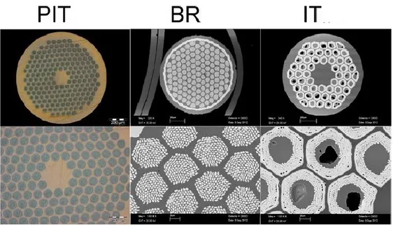
Practical superconducting wires are made in composite form, containing both superconductor and a normal conductor. Indeed, heat transfer through the conductor is the main channel for removing heat and, consequently, preventing a quench. In particular, technical superconductors for large-scale applications are round or tape-shaped wires in which one or more superconducting filaments are embedded in a matrix consisting at least partially of a normal metal, such as Cu or Ag. They must carry operating currents, DC or AC, of hundreds of amperes. Among several superconducting elements and compounds, only a few of them are technologically suitable from the point of view of manufacturing wires for the current transport applications [3]. The currently commercial superconducting materials are NbTi, Nb3Sn, Bi2Sr2CaCu2O7 (Bi-2212), Bi2Sr2Ca2Cu3O10 (Bi-2223), MgB2, and YBa2Cu3O7.

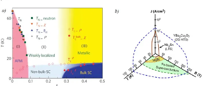
Nowadays, the improvement in the fabrication techniques of iron-based superconductors have made them real competitors of HTS and MgB2 in the perspective of high power wires and/or tapes production. Among the families of iron-based superconductors, the 11-family is one of the most attractive for high field applications at low temperatures.It has been recently demonstrated that it is possible to realize coated conductors able to carry very high current densities (up to 105 _{A cm}-2 _{at 4.2 K and 30 T) [15] and it is} possible to improve further the critical current density value with the proper choice of the substrate [16-18].

7

What we have done

We have carried out electrical and thermal transport characterization on superconducting materials relevant for applications and technical superconductors, as well. Measurements of this work were performed at MaSTeR-Lab of CNR-SPIN Salerno and Physics Department of Salerno University. The electrical transport characterization of 11-compound Fe(Se,Te) thin films uses cryogen-free measurement systems. The Fe(Se,Te) thin films studied belong to the second generation of high-quality and purity thin films grown on CaF2 substrates. All samples are provided by CNR-SPIN Genova. The obtained results have been compared with the first-generation one [18].

The analysis of the Fe(Se,Te) thin films R(T) curves, carried out at fixed values of magnetic field, has allowed to estimate the pinning activation energy U. The pinning force as a function of the magnetic field has been also evaluated by Jc measurements, that is evaluating the maximum current value above which

dissipation sets in. Then, by using the Dew-Hughes approach we have analyzed the pinning centers landscape.

However, the use on a large scale of iron-based cannot be achieved without the understanding of the current stability mechanisms in these compounds. For this reason, we have studied the I-V curves in a regime well above the critical current Jc and quench features similar to those related to FFI have been

recognized.

A preliminary study has been done to determine how the instability parameters are influenced by the cooling environment. Indeed, cooling efficiency and thermal stability are strictly demanding for practical applications of superconductors operating at current values close to the critical current Ic, because a thermally unstable device can show premature quench. To obtain thermal stability, a balance between heat removal from the material and Joule heating must be reached. To this aim, we have studied heat exchanges of superconducting samples with the surrounding environmental setup by current driven stability measurements. In particular, we analyse I-V characteristics up to current values triggering the instability of the flux flow regime on NbN and NbTiN ultra-thin films realized in collaboration with CNR-SPIN Salerno and CEA Grenoble (J. C. Villégier Group).

The ultra-thin films have been cooled in different environments, namely liquid Helium bath and cryogen-free system with both dynamic He-gas and static He-gas. The effects of the cooling method on the electric current carrying stability of NbN and NbTiN ultra-thin films are reported.

It has been also investigated the relation between the critical current and the instability current in Fe(Se,Te) microbridges, with the analysis focus on the difference I*−Ic , which can be seen as a safe range

before the full quench of the superconductor. Indeed, in the range between Ic and the instability current

I*, the material is still in the superconducting phase, but dissipation due to moving vortices is present.

8 applications of superconducting materials, but less well studied in the community, with few works on HTSs to our knowledge [19-20].

Experimental studies involving technical superconductors Bi2Sr2CaCu2O8+x (Bi-2212) round wires are

performed in collaboration with the Group of Applied Superconductivity (C. Senatore Group) at “Département de Physique de la Matière Quantique” of Geneva University (Switzerland). The thesis work is focused on electrical and thermal characterization of superconducting wires manufactured by Oxford Superconducting Technology (OST).

We have studied the thermal stability of technical superconductors by means of thermal and electric transport measurements. An increase of mass density, electrical connectivity and critical current density has been obtained in the samples by overpressure process under different total pressures reached adding Ar at a fixed O2 partial pressure of 1 bar, with a maximum T of 890° C [21-

25]. In particular, the thermal conductivity κ of samples reacted at different pressures, namely 1, 10 and 100 bar, in magnetic fields up to 19 T, have been examined.

An open issue about Bi‐2212 conductors is understanding to what extent the Ag matrix is contaminated during the heat treatment due to Bi‐2212 element diffusion. Among the elements composing Bi‐2212, Cu has the highest solubility in Ag [26]. This contamination could have a negative effect on the RRR value and, consequently, on the thermal conductivity of the whole wire. Contrary to the case of LTS, the RRR of the matrix in HTS technical conductors cannot be evaluated from a resistivity measurement performed on the whole conductor. Indeed, due to the superconducting transition at high T, it is not possible to measure the residual ρ of the matrix. Previously, the residual resistance ratio (RRR) of the matrix had been evaluated in Bi-2212 wires processed with a non-standard partial-melt-processing in order to depress the critical current of the samples with very little superconducting phase [26]. In this work, an alternative method is presented which overcomes previous critical results [26]. Here the RRR of the metal matrix has been estimated by measuring the electrical resistance of short pieces of conductor in which the superconducting filaments have been removed by chemical etching. In this way, the samples are not exposed to heat treatments that could change the degree of contamination of the matrix. This has allowed us to quantify the effects of the overpressure heat treatment on the low-temperature electrical and thermal conductivity properties.

Moreover, a preliminary study on NZPV is presented. Among the various models known to estimate the

NZPV the approximated expression used for the REBCO CC was taken into consideration. We have

evaluated the error committed in this procedure for the NZPV estimate, measuring the heat capacity C(T) of the Bi-2212 round wires, and we have been able to determine how the error is reduced as the magnetic field increases.

9

Structure of this PhD Thesis work

The present work is constituted by four Chapters.

In the first part of Chapter 1, we present an overview on general aspects of superconductivity and the fundamentals on type II superconductors, pinning mechanisms and vortex dynamics in superconducting materials also introducing the parameters relevant for thermal stability of superconducting devices. Then, we present the superconducting materials that are relevant from the point of view of the applications. Finally, technical superconductors and their thermal transport properties are discussed.

In Chapter 2, the reader can find an overview on cooling methods as well as information about the measurements setups and the samples preparation.

In Chapter 3, the results of the electrical transport properties on Iron-based thin films are shown. Moreover, a study on the efficiency of cooling methods by FFI measurements on Nb-based thin films is also shown.

In Chapter 4, the determination of the thermal conductivity κ, heat capacity C(T) and of RRR by means of thermal and electrical transport measurements is reported.

11

1 SUPERCONDUCTIVITY AND APPLICATIONS

1.1 General Aspects

Superconductivity is a state of matter characterized by perfect conductivity and perfect diamagnetism [27]. It was discovered by H. Kamerlingh Onnes in 1911 when, while he was investigating the low temperature electrical resistance of a mercury sample, he found that below 4.15 K the DC resistance of that element decreased suddenly to zero [28]. In the following years, superconductivity was found in many metals, metallic compounds and alloys each of one showed superconductivity below different temperature values. The temperature below which their resistance drops to zero is called critical temperature and usually denoted as Tc. In 1933, Meissner and Ochsenfeld discovered the second effect, perfect

diamagnetism, when they found that superconductors completely expelled internal magnetic fields below a certain critical field value, Hc [29].

Two years later, the London brothers developed a model based on two phenomenological equations explaining the Meissner effect and providing the penetration depth of the external magnetic field into the superconductors [30]. Subsequently, in 1950, Ginzburg and Landau formulated the so called macroscopic theory of superconductivity describing the superconducting state through an order parameter and providing a derivation for the London equation. In 1957, thanks to Ginzburg-Landau (GL) theory, A. Abrikosov explained some experimental observations concluding that for some superconductors there are two critical fields, Hc1 and Hc2, among which there exists a mixed state where magnetic field penetrates

the superconductor in quantized flux lines [31]. Superconductors showing only the Meissner state are referred as Type-I, while those also showing the mixed state are of Type-II. In the same year, Bardeen, Cooper and Schrieffer (BCS) introduced a microscopic theory of superconductivity [32]. BCS theory shows that superconductivity is due to the condensation induced by phonon interactions of electrons pairs (Cooper pairs) into a coherent ground state and that superconducting and normal state are divided by an energy gap. Both Ginzburg-Landau and London equations well fit into BCS formalism and many of its predictions were confirmed by experiments.

Following a BCS Theory interpretation, it has been argued that lattice instabilities would have destroyed Cooper pairing preventing any material to show a critical temperature higher than 30-40 K [33]. In spite of this prediction, in 1986 Alex Müller and Georg Bednorz discovered superconductivity in a sample of LaBaCuO with a critical temperature about 30 K [34]. This discovery was surprising because this material is a ceramic oxide that is typically an insulator. Due to that discovery the research on superconducting materials was mainly focused on copper oxide (cuprate) compounds bringing in a few years to a Tc of

about 90 K (above the boiling point of liquid N2 at 77 K) found in the cuprate YBa2Cu3O7-δ. [35-36]. In the following years, many different cuprate systems showed such high transition temperature reaching the

12 critical temperature of 138 K at atmospheric pressure and 164 K under 30 GPa in the HgBa2Ca2Cu3O8 compound [37]. Many properties of these high-temperature superconductors (HTSC) are highly unusual. More than 25 years after their discovery, it is still unclear how the Cooper pairing is accomplished in these materials and it seems likely that magnetic interactions play an important role. The BCS theory is unsuitable to describe superconductivity in these complicated materials and the mechanism of high-temperature superconductivity is still an open question.

In 2001, the superconductivity was discovered in the compound MgB2, synthesized for the first time in

1953 [38]. For years it has been considered a conventional superconductor, with the highest critical temperature (Tc = 39 K) found until then, but the presence of a gap multiband structure makes it not

completely explained by the BCS theory [39-40].

In 2008, H. Hosono et al. discovered another superconducting family, the iron based. They first found that the LaO1−xFxFeAs compound was superconductor at 26 K [41]. Moreover, its critical temperature can

reach higher Tc replacing Lanthanum atoms with other rare earth elements such as cerium, neodymium and praseodymium and up to 56 K with samarium doping [42-44]. In the iron base family are included iron-chalcogenides with the best critical temperature around 50 K [45]. Recently it was found that in particular conditions of growth on suitable substrates it was possible to obtain a Tc up to 100 K for FeSe-based ultra-thin films [46-47].

Several guidelines for achieving high Tc with no upper limit have been theorized in the past years (see also Fig. 1.1, [48]). For example, referring to the BCS Theory, Ashcroft argued that conditions as high-frequency phonons, strong electron–phonon coupling, and a high density of states, which can be in principle satisfied by metallic hydrogen and hydrogen dominant metallic alloys, can lead to Tc up to 300 K [49-51]. Indeed, in 2015, Drozdov et al. found that sulphur hydride transforms to a metal at a pressure

Fig. 1.1 : Superconducting timeline, BCS superconductors are displayed as green circles, cuprates as blue diamonds, and iron-based superconductors as yellow squares [48].

13

of approximately 90 GPa and shows superconductivity transition at a Tc of 203 K at a pressure of 150 GPa just by following these guidelines [52]. Through this discovery, this material class is thought to be the best candidate to achieve room-temperature superconductivity.

1.1.1 Fundamentals

The phenomenological Ginzburg-Landau theory focuses its predictions entirely on the superconducting electrons providing that the local density of superconducting electrons nsc is represented by the

introduction of a complex pseudo-wavefunction, referred as the order parameter ψ(r), for which holds the

relation |𝜓(𝑟⃗)|2_{= 𝑛}

𝑠 [27, 53].

The order parameter ψ(r) is the solution of the differential equation obtained using a variational principle

starting from a series expansion of the free energy in power of ψ and ∇ψ with expansion coefficients α

and β which takes the form:

1 2𝑚∗(−𝑖ℏ𝛻⃗⃗ − 𝑒∗ 𝑐 𝐴⃗) 2 𝜓 +𝛽 2|𝜓| 2_{𝜓 = −𝛼𝜓 (1. 1)}

where m* and e* are the Cooper pair mass and electric charge respectively, β must be positive for validity of theory, while α can be positive or negative. If α > 0, the minimum free energy corresponds to:

| 𝜓|2 _{= 0}

If α < 0, the minimum free energy corresponds to:

| 𝜓|2 _{= | 𝜓}

∞|2= −

𝛼

𝛽 (1. 2) here 𝜓_∞ is the maximum concentration of Cooper pairs that can exist infinitely deep in the interior of the superconductor completely shielded from any field or current [27]. The characteristic distance over which

ψ(r) can vary without relevant energy increase is the so-called coherence length

𝜉(𝑇) = ℏ

[2𝑚∗_𝛼(𝑇)]1 2⁄ ∝

1

√1 − 𝑇 𝑇⁄ _𝑐 (1. 3) Another characteristic length is the magnetic penetration depth λ(T), which characterizes the distance over which the magnetic field is screened by the superconducting currents. It is found by II London equation [27]:

ℎ⃗⃗ = −𝑐𝛻⃗⃗ × 𝛬𝐽⃗_𝑠 (1. 4) where h denotes the value of magnetic field density on a microscopic scale and 𝛬 = 4𝜋𝜆2 _𝑐2_{= 𝑚 𝑛}

𝑠𝑒2

⁄

⁄ .

14 𝛻2ℎ⃗⃗ = ℎ⃗⃗ 𝜆2 (1. 5) 𝛻2_𝐽⃗ 𝑠= 𝐽⃗_𝑠 𝜆2 (1. 6) Where 𝜆 = √𝛬 𝜇⁄ ₀= √ 𝑚𝑐 2 4𝜋𝑛_𝑠𝑒2 (1. 7)

is called the London penetration depth. The solutions of these differential equations, in turn, yield magnetic fields and currents that, from their value on the superconductor surface, exponentially decrease with the London penetration depth λ inside the material. The penetration depth λ is temperature dependent due to the nsc temperature dependence. The temperature dependant λ(T) was found to be approximately

[27]: 𝜆(𝑇) ≈ 𝜆(0) [1 − (𝑇 𝑇⁄ )𝑐 4] 1 2 (1. 8)

It is useful to introduce the dimensionless Ginzburg–Landau parameter κ, which is defined as the ratio of the two characteristic lengths

𝜅 ≡𝜆(𝑇)

𝜉(𝑇) (1. 9)

In pure superconductors, 𝜅 ≪ 1, but in dirty superconductors or in HTS, 𝜅 ≫ 1.

Superconductors can be classified on the basis of their Ginzburg-Landau parameter value. Type I superconductors are those with 𝜅 < 1 √2⁄ with a positive sign of the surface energy of a boundary between normal and superconducting regions, while type II superconductors have 𝜅 > 1 √2⁄ and a

Fig. 1.2: Schematic diagram of variation of h and ψ in a domain wall. The case κ«1 refers to a type I superconductor; the case κ»1 refers to a type-II superconductor [27].

15 negative surface energy, which favours the formation of superconducting-normal boundaries and magnetic flux penetration [31].

The H − T phase diagram for a bulk type I and type II superconductor is represented in panels (a) and (b) in Fig. 1.3, respectively. Type I superconductors (𝜅 < 1/ √2) are in the Meissner state for applied fields up to Hc, given by

𝐻𝑐(𝑇) =

𝛷₀

2√2𝜋𝜇0𝜆(𝑇)𝜉(𝑇)

(1. 10)

where Φ0 is the superconducting flux quantum (see below). In the Meissner state, all magnetic flux is expelled from the interior of the sample (B = 0). At Hc(T) a first-order transition occurs leading to a

discontinuous breakdown of superconductivity, and the sample turns to the normal state [Fig. 1.3(a)]. Type II superconductors (𝜅 > 1/ √2) are in the Meissner state for fields smaller than the first (or lower) critical field

𝐻_𝑐1(𝑇) = 𝛷0

4𝜋𝜇₀𝜆2_(𝑇)𝑙𝑛(𝜅) (1. 11)

For fields H > Hc1(T), there is a penetration of magnetic flux until, at the so-called second (or upper)

critical field, the system becomes normal [Fig. 1.3 (b)]. This second critical field can be expressed as

𝐻_𝑐2(𝑇) = 𝛷0 2𝜋𝜇0𝜉2(𝑇)

(1. 12)

The phase between Hc1 and Hc2 is referred as mixed state or Abrikosov vortex state, where the flux

penetrates in a regular array of flux tubes or vortices, each bearing a superconducting flux quantum Φ0=

ℎ/2𝑒 = 2.07 × 10−15 _{T m}2 _{[31]. Thanks to the partial flux penetration, the diamagnetic energy for} maintaining the field out is less, so Hc2 can be much greater than Hc.

16

1.1.2 Vortex lattice

The magnetic field penetrates in a type II superconductor as an array of vortices distributed through the material. If the separation between the vortex is large compared to λ, the vortex-vortex interactions can be neglected, then they can be considered as isolated. The vortex structure consists of a normal core of radius ξ, around which shielding currents circulate. The local magnetic field h and the superconducting electron density nsc are functions of the distance r from the vortex center as schematically represented in

Fig. 1.4 [54].

The local magnetic field and current distribution in the mixed state (Hc1 < H < Hc2) of a type II

superconductor can be calculated from the London model [30], with the requires of 𝜅 ≫ 1 and the order parameter is nearly constant in space. In this limit, we can obtain from London equation (1.4) the local field distribution around a vortex as [27]

𝜇₀ℎ(𝑟) = 𝛷0 2𝜋𝜆2𝐾0(

𝑟

𝜆) (1. 13) where K0 is the zero-order Bessel function which, at short distances (𝜉 < 𝑟 ≪ 𝜆), tends to:

𝐾0= 𝑙𝑛 (

𝜆

𝑟) (1. 14) and, at large distances (𝑟 ≫ 𝜆), tends to:

𝐾0 = √

𝜋𝜆

2𝑟𝑒𝑥𝑝 (− 𝑟

𝜆). (1. 15)

Fig. 1.4: Structure of a single vortex, showing the radial distribution of the local field h(r), the circulating supercurrents j(r) and the density of superconducting electron nsc(r) [54]

17 It can be observed that the local field h is highest in the center of the vortex core where superconducting order parameter (ψ or nsc) is zero and his value is given by the limiting form:

𝜇₀ℎ(𝑟) ≈ 𝛷0 2𝜋𝜆2[𝑙𝑛

𝜆

𝑟+ 0.12] , 𝜉 ≪ 𝑟 ≪ 𝜆 (1. 16) and decays over a distance given by the penetration depth λ:

ℎ(𝑟) → 𝛷0 2𝜋𝜆2( 𝜋 2 𝜆 𝑟) 1 2⁄ 𝑒−𝑟 𝜆⁄ _{, 𝑟 → ∞ (1. 17)}

due to the screening currents. Then, the current distribution of a single vortex can be calculated by performing the derivative of the local field with respect to the radial distance dependence, [55]:

𝐽(𝑟) = 𝛷0 2𝜋𝜇₀𝜆2𝐾1(

𝑟

𝜆) (1. 18)

Here, K1 is the first order Bessel function which decreases as 1/r for 𝜉 < 𝑟 ≪ 𝜆, and diverges as K0 at

large distances 𝑟 ≫ 𝜆. Finally, the energy of a flux line is the sum of the field and the kinetic energy of the currents and a small core contribution [56]:

𝐸𝑙 = 1 4𝜋𝜇₀( 𝛷₀ 𝜆 ) 2 [𝑙𝑛 (𝜆 𝜉) + 0.12] (1. 19)

where the constant 0.12 describes the contribution of the normal core. Since El is a quadratic function of

the magnetic flux, it is energetically unfavourable in a homogenous superconductor to form multiquanta vortices, carrying more than one flux quantum.

The interaction energy between more parallel vortices is easy to treat under the approximation 𝜅 ≫ 1. Due to the repulsive electromagnetic interaction, they tend to be positioned as far away from each other as possible, resulting in the well-known Abrikosov vortex lattice [31]. The repulsive force between two vortices fij is [56]: 𝑓_𝑖𝑗(𝑟_𝑖𝑗) = 𝛷0 2 2𝜋𝜇₀𝜆3𝐾1( 𝑟_𝑖𝑗 𝜆) (1. 20)

18 If two vortices are generated in a type I superconductor, the value of ξ is larger than λ, so the normal cores overlap first, leading to a gain in the condensation energy and thus to vortex-vortex attraction [57] [58] [Fig. 1.5(a)]. Instead in a superconductor of the type II, the magnitude of the λ value would cause the

currents to overlap first, leading to vortex-vortex repulsion [Fig. 1.5(b)]. For a given vortex density, the most favourable configuration in which the vortices are arranged is triangular lattice [Fig. 1.6], with the density of vortices nv increases with increasing field. The distance av between nearest neighbour vortices

in the triangular lattice is related to the induction B through the relation

𝐵 = 𝛷0𝑛𝑣=

2 √3

𝛷0

𝑎_𝑣2 (1. 21)

Fig. 1.5:Schematic diagram of a triangular vortex lattice with period av, The dashed lines indicate the unit cells [54].

Fig. 1.6: Schematics of the vortex-vortex interactions: (a) in type I superconductors, vortex core are overlapping first, thus causing an attraction between vortices; (b) in type II materials, the first to overlap are the local fields h(x), which leads to a vortex-vortex repulsion [54].

19

1.1.3 Vortex Pinning

In the case that a Type II superconductor immersed in a magnetic field above Hc1 is crossed by an electric

current, the flux lines start moving due to the Lorentz force that results from the action of the current density J⃗ on the flux lines. Such a Lorentz force per unit length and per one vortex is given by:

𝑓⃗_𝐿 = 𝐽⃗ × 𝛷⃗⃗⃗₀ (1. 22)

and tends to move the vortices transversely to the current. Such motion induces an electric field parallel to J⃗ of magnitude:

𝐸⃗⃗ = 𝐵⃗⃗ × 𝑣⃗ (1. 23)

where 𝑣⃗ is the flux lines velocity. This acts like a resistive voltage with power dissipation and, in this scenario, makes a type II superconductor to be unable to sustain a persistent current.

In order to be suitable for applications, type II superconductors must be able to carry high current in very high fields without resistance. In other words, there should be a threshold current value below which no power dissipation is observed. High values for such a critical current density can be reached if the flux lines are prevented from moving. Thus, a pinning force 𝑓⃗_𝑃 associated with the introduction of a pinning center into the superconductor should neutralize 𝑓⃗L. In real type-II superconductors, vortices are pinned

by any spatial inhomogeneity of the material causing a local minimum in the free energy landscape. Crystalline imperfections, columnar defects, grain boundaries, twin boundaries, or stochiometric deviations, amongst others, can act as pinning centers. The pinning can also be induced artificially by irradiation, ion implantation, film thickness modulation, doping, etc.

However, if currents are strong enough, and the pinning is weak compared to the driving force a regime sets in, in which the vortex moves. In the flux flow regime, the vortex velocity can be though as limited by a viscous drag. In this scenario, the total force acting on the flux line per unit length is the sum of several contributions [59]:

𝑓⃗ = 𝑓⃗_𝐿− 𝑓⃗_𝑃− 𝜂𝑣⃗_𝑣− 𝑓⃗_𝑀 (1. 24)

where −𝜂𝑣⃗𝑣 is a small friction-like contribution (the viscous damping force) proportional through η to the

vortex velocity 𝑣⃗_𝑣, and 𝑓⃗_𝑀= 𝛼(𝑣⃗_𝑣× 𝑛̂) is the Magnus force, where 𝑛̂ is a unit vector in magnetic field direction and α a constant. As long as every individual vortex is prevented from moving, for the eq. (1.25) it holds the condition 𝑓⃗ = 𝑓⃗_𝐿− 𝑓⃗_𝑃 = 0. As the bias current increases, the Lorentz force will reach a value equal to the pinning force, beyond which the vortices will undergo a depinning. The current value for

20 which this condition is reached is the critical current Ic, also referred as depinning current. The average macroscopic pinning force per unit volume is related to the depinning current density by the expression

𝑓𝑃= 𝐽𝑐𝐵 (1. 25)

In a steady state, the vortex velocity 𝑣⃗_𝑣, will achieve a constant value. In the limit of a pinning-free superconductor (𝑓_𝑃 = 0), 𝑣⃗_𝑣 is determined entirely by the viscosity of the medium, yielding 𝑣⃗_𝑣 = (𝑱 × Φ0) 𝜂⁄ . From this expression, and from eq. (1.24) it is possible to define the flux flow resistivity [27]

𝜌𝑓 =

𝐸 𝐽 = 𝛷0

𝐵

𝜂 (1. 26)

which arises exclusively from the viscous flow of vortices.

The critical current density may be determined experimentally as function of B. From eq. (1.25), the resulting 𝑓_𝑃(𝐵) function shows a maximum in the 𝑓_𝑃(𝐵) function, being zero at 𝐵 = 0 and at 𝐵 = 𝜇₀𝐻_𝑐2 due to 𝐽_𝑐(𝜇₀𝐻_𝑐2) = 0 for definition. Introducing the normalized magnetic field (ℎ = 𝐻 𝐻⁄ _𝑐2), it is found that at different temperature

𝑓_𝑃(ℎ) ∝ 𝐻𝑐2𝑛(𝑇)𝑓𝑛(ℎ) (1. 27)

where n and 𝑓𝑛(ℎ) are characteristic of the pinning mechanism operating in the superconductor.

Among the theories which have tried to account for the observations about pinning properties in materials, Dew-Hughes approach has a good general view [60]. In this approach, the pinning force per unit volume is expressed as:

𝑓_𝑃 = −𝛾𝐿∆𝑊

𝑥 (1. 28) where ΔW is the work done to move a unit length of flux-line from a pinning center to the nearest position where is unpinned, x is the effective range of pinning interaction, L is the total length of flux-line per unit volume which is directly pinned and γ is an efficiency factor determined by the extent to which the flux-line neighbours in the lattice allow to relax toward a position of maximum pinning. These quantities are influenced by the nature and the size of the pinning centers, the rigidity of the flux line lattice and the size of the pinning micro-structure compared to λ, intimately connected to fundamental nature of the pinning interaction. Fundamental pinning interactions are the ones between the normal core and a pinning site (core interactions), or the interactions between the pinning sites and the distribution of magnetic fields and supercurrents in the sample (magnetic interactions). The analytical expressions for the 𝑓_𝑛(ℎ) in the various cases can be summarized as in Table 1.1 and sketched as in Fig. 1.7.

21 Regarding the behaviour of the vortex lattice in the presence of pinning forces, assuming a certain elasticity of the lattice, two cases can occur. In the first case, the pinning force exerted by the pinning sites is weak and so the lattice preserves its long range correlation, in the second one, the pinning force is so strong that the breaking of the lattice structure is possible. These possibilities as referred as weak pinning and strong pinning respectively [27, 61]. The action of many weak pins on the vortex system is described by the collective pinning theory while the interaction between vortices and strong pinning center is described by Labusch model. The crossover between weak and strong pinning is based on defining the Labusch criterion [62]:

𝑓_𝐿𝑎𝑏 =𝜖0𝜉

𝑎₀ (1. 29)

where 𝜖₀= 𝛷_0⁄4𝜋λ2 _{is the line energy scale. In weak pinning regime 𝑓}

𝑃< 𝑓𝐿𝑎𝑏, while the strong pinning

regime is characterized by 𝑓𝑃> 𝑓𝐿𝑎𝑏.

The vortex pinning and the condition J < Jc do not warrant the complete absence of vortex motion. Indeed,

thermal excitations can provide enough energy for vortices to hop from one pinning site to another at Table 1.1

22 finite temperatures. This type of vortex motion generates a resistive voltage proportional to the average creep velocity. This regime is referred as flux creep, and its velocity is usually much smaller than the resistive flux flow velocity. In the Anderson-Kim Flux-Creep theory, which assumes flux line bundles jumping as a unit due the interaction between vortex, the electric field generated by the flux-creep-assisted vortex motion is given by [27]

𝐸 = 𝑣 ∙ 𝐵 = 𝜔₀𝐿 ∙ 𝑒− 𝑈0 𝑘𝐵𝑇∙ 𝑠𝑖𝑛ℎ (𝛼𝐿 4 𝑘𝐵𝑇 ) (1. 30)

Here v is the creep velocity, ω0 is a characteristic frequency of flux-line vibration ranging within 105 _to 1011 _s-1_{, L is the jump width, α is the driving force density so that αL}4 _{is the difference in potential energy}

between two neighbouring pinning sites, and U0 = U0 (T, B, J) is the activation energy or barrier energy,

i.e. the height of the potential barrier between two adjacent pinning sites. For 𝐽 ≪ 𝐽_𝑐𝑘𝐵𝑇

𝑈0, the system is in the so-called thermally assisted flux flow (TAFF) regime where for the electric field it is possible to write:

𝐸_{𝑇𝐴𝐹𝐹} ∝ 𝐽 ∙ 𝑒𝑥𝑝 [− 𝑈0 𝑘𝐵𝑇

23

1.1.4 Flux Flow Instability

The equation (1.26), obtained neglecting flux pinning, showed the Ohm’s law behaviour 𝐸 ∝ 𝐽 of free flux flow regime. However, the constancy of the dumping η and the Magnus force α coefficients require that the vortex structure does not change. This scenario is reasonable at low vortex velocity, while at high vortex velocity strong deviation from linear Ohm’s law can be observed.

This kind of non-linear flux flow behaviour can be explained through the Larkin-Ovchinnichov (LO) theory which assumes spatial homogeneity of the nonequilibrium quasiparticle distribution [63]. In the high temperature limit (𝑇 ≈ 𝑇_𝑐), where the order parameter is most sensitive to small changes in quasiparticle distribution function, the vortex core is approximated by a normal phase cylinder with radius ξ filled with quasiparticles [11]. The electric field generated by vortex motion provides to the quasiparticle energy sufficient to get out of the core. As a consequence, a fraction of the quasiparticles leaves the vortex core, thus the core shrinks and the damping coefficient of the friction force η𝑣_𝜑 decreases with increasing vortex velocity 𝑣𝜑.

The relation derived by LO for the damping coefficient is

𝜂(𝑣_𝜑) = 𝜂(0) 1 + (𝑣𝜑⁄𝑣𝜑∗)

2=

𝜂(0)

1 + (𝐸 𝐸_⁄ ∗₎2 (1. 32)

Here η(0) is the damping coefficient in the limit 𝑣_𝜑 → 0 while 𝑣_𝜑∗ _{is the velocity value above which we}

have a negative differential resistivity. This critical velocity 𝑣𝜑∗ can be expressed as:

𝑣𝜑∗ 2 =

𝐷[14𝜁(𝑥 = 3)]1 2⁄ _{(1 − 𝑇 𝑇} 𝑐

⁄ )1/2

𝜋𝜏_𝜀 (1. 33)

where 𝐷 = 𝑣_𝐹𝑙 3⁄ (with 𝑣_𝐹 the Fermi velocity and l the electron mean free path) is the diffusion coefficient of the quasiparticles, 𝜁(𝑥) = ∑ 1

𝑛𝑥

∞

𝑛=1 is the Riemann zeta function and 𝜏𝜀 is the quasiparticle energy

relaxation time. The relation between the critical voltage V* and the velocity 𝑣_𝜑∗ _{is [12]:}

𝑉∗_{= |𝑣⃗}

𝜑∗× 𝐵⃗⃗|𝐿 = 𝜇0𝑣𝜑∗𝐻𝐿 (1. 34)

where L is the length of the current path between the voltage contacts and H is the applied magnetic field. In agreement with LO model the current-voltage characteristics is described by the relation [12]:

𝐼 − 𝐼_𝑐 = 𝑉 𝑅𝑓𝑓 [ 1 1 + (𝑉 𝑉_⁄ ∗₎2+ 𝑐 (1 − 𝑇 𝑇𝑐 ) 1 2⁄ ] (1. 35)

24 Where Ic is the critical current and 𝑅𝑓𝑓 is the flux-flow resistance and c is a constant of order unity. At

𝑉 = 𝑉∗_{, the corresponding current value I* is the instability current at which the negative differential}

resistance appears. This branch, subsequently, merges the normal state branch V = RNI (in which RN is the

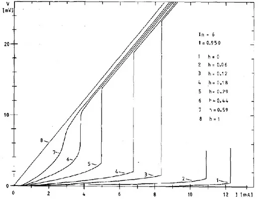
normal state resistance). In the current-driven measurements the S-shaped curve is hidden by an abrupt jump from flux flow regime to the normal state branch at I = I*. This sudden voltage jump, also referred as quench, is the signature of the Flux Flow Instability (FFI) phenomenon. I-V curves of a Nb film, for different values of the magnetic field at T = 4.2 K, displaying the voltage jumps, are shown in Fig. 1.8. Although from (1.30) the critical velocity 𝑣𝜑∗ is expected independent of the magnetic field B, it has been

experimentally found that at low magnetic fields 𝑣_𝜑∗_~𝐵−1/2 _[64].

In the low-temperature limit (𝑇 ≪ 𝑇_𝑐), the electronic instability can be related to the electron overheating [65-66]. Due to dissipations in the flux-flow regime, electrons reach temperatures above the phonon temperature, which leads to an expansion of the vortex core and a consequent reduction of the viscous drag. The signature of the instability in the I -V curves is very similar between the LO as in the electron overheating regime, despite the different mechanisms present in the two distinct temperature ranges.Also, the magnetic field dependence of the critical vortex velocity is 𝑣∗ _{∝ 𝐵}−1_{2 [65], although it has been noted}

that, regardless of the temperature limit, a more complex dependence can be present at very low fields, due to the pinning properties of the material and sample geometry [67-72].

Fig. 1.8: Voltage-current characteristics for a superconducting thin film of In, grown on a sapphire substrate, at different applied magnetic fields. [11]

25 The quenching of the superconducting state can also occur due to the Joule self-heating caused by thermal dissipations of the vortex motion. The occurrence of this thermal instability in HTSCs at zero applied

magnetic field has been theoretically described as a pure consequence of a temperature runaway, which takes place up to the quenching temperature T∗_{, where a very steep voltage jump sets in [73-74]. It is} claimed that, under certain experimental conditions heating effects become predominant [73], and at sufficiently high current densities cuprate HTSCs become thermally unstable [74]. In Fig. 1.9 is illustrated an experimental procedure where the I-V curves obtained are not constant temperature curves [73]. On the other hand, also the LO model has been extended by Bezuglyj and Shklovskij [11] (BS) in order to include the effect of self-heating near Tc in a finite magnetic field. In this case, a crossover scenario

emerges with a threshold value of the applied magnetic field BT between the LO and pure self-heating

regimes. For 𝐵 ≪ 𝐵𝑇 the instability is triggered by an intrinsic change of the distribution function of

quasiparticles trapped in the vortex core, whereas for 𝐵 ≫ 𝐵_𝑇 it is driven by pure thermal effects [75].

This crossover corresponds to a distinctive magnetic-field dependence of the Joule power 𝑃∗_{= 𝐼}∗_𝑉∗ _at

the instability, which is field dependent for 𝐵 ≪ 𝐵𝑇 and saturates for 𝐵 ≫ 𝐵𝑇.This parameter is expressed

in terms of the quasi-particle energy relaxation time 𝜏_𝜀 and the heat transfer coefficient h as:

𝐵𝑇 =

0.374 ∙ 𝑒 ∙ ℎ ∙ 𝜏𝜀

𝑘_𝐵 (𝑅𝑁

𝑊

𝐿) (1. 36) with kB the Boltzmann constant, e the electron charge and RN the normal state resistance at Tonset, W is the

width and L the length of the superconductor.

In general, the relative importance of thermal effects can be characterized by the value of the Stekly parameter α [76], defined as the ratio of the heat generation in the normal state 𝜌_𝑁𝐽_𝑐2 _{and the heat transfer}

2(𝑇𝑐− 𝑇)ℎ/𝑑, being ρN, Jc, h, and d, respectively, the normal state resistivity, critical current density,

Fig. 1.9: Experimental building procedure I-V curves with a staircase ramp of current applied to YBCO microbridges [73].

26 heat transfer coefficient, and film thickness [76]. Self-heating is important if 𝛼 > 1, and negligible if 𝛼 ≪ 1. This parameter gives a measure of thermal contributions to the flux flow instability, and depends on the intrinsic properties of the sample, but also on experimental conditions and on the substrate.

1.1.5 T

, H

, J

: Critical Surface

In practical applications, superconducting materials biased by an electric current often must work in high magnetic fields. Therefore, let us analyse the behaviour of a cylindrical superconducting wire immersed in a magnetic field parallel to its axis. The superconducting perfect diamagnetism involves that within the superconductor the magnetic field is zero (Bin = 0), while on the surface it is equal to the external value

(Bext = µ0Hext). Moreover, Ginzburg–Landau and London theories provide the presence of a layer at the

lateral surface of superconductor where the magnetic field drops exponentially to zero from its external value on a distance equal to the penetration depth. In this layer, a shielding current circulates to generate an inner field opposite to the external field which cancels the field inside the superconductor. We must also consider that when an electric current bias is applied to the wire, it generates a radial magnetic field with a linear radius dependence inside it and inversely proportional dependence outside it. Moreover, the current density cannot be uniform inside it, otherwise internal magnetic flux would be different from zero, but it must flow only in the λ spaced surface layer, perpendicular to the shielding current. Both for the shielding current and for the transport current we have that the current density is given by [55]:

𝐽(𝑟) =𝐵𝑠𝑢𝑟𝑓 𝜇₀𝜆 𝑒𝑥𝑝 [− (𝑅 − 𝑟) 𝜆 ] = 𝐼 2𝜋𝑅𝜆𝑒𝑥𝑝 [− (𝑅 − 𝑟) 𝜆 ] (1. 37) Where Bsurf is the magnetic field at surface of wire, R is the wire radius, r is the radial distance from the

wire centre. The total current is obtained by integrating J(r) over the cross section of the superconducting wire and is I = 2πRλJ where 2πRλ is the effective cross-sectional area of the surface layer and J is J(r) calculated at r = R.

In the case of superconductors, the fact that there is a critical field Hc also limits the amount of maximum current that can flow within it. For both the shielding and the transport case we have

𝐵_𝑐(𝑇) = 𝜇0𝜆(𝑇)𝐽𝑐(𝑇) (1. 38)

Here the current value Jc is the value of the current at which the critical field Hc is reached. In Type I

superconductors, where current can flow only in a surface layer of thickness λ, the average current density carried by a superconducting wire with R >> λ is very low. It would be possible to obtain high average current densities if the radius R is less than penetration depth. The fabrication of such filamentary wire is not practical since Type I superconductors show a λ about 50 nm.

The explicit temperature dependences of Bc(T) and λ(T) and 𝐽𝑐(𝑇) = 𝐵𝑐(𝑇) 𝜇⁄ 0𝜆(𝑇) are given by

27 𝐵𝑐= 𝐵𝑐(0) [1 − ( 𝑇 𝑇_𝑐) 2 ] 𝜆 = 𝜆(0) [1 − (𝑇 𝑇𝑐 ) 4 ] −1 2⁄ 𝐽𝑐 = 𝐽𝑐(0) [1 − ( 𝑇 𝑇_𝑐) 2 ] [1 − (𝑇 𝑇_𝑐) 4 ] −1 2⁄ (1. 39)

Where λ(0) = λL. The asymptotic behaviours at T→0 K [77] and near the transition temperature T ≈ Tc

[78] were found respectively as:

𝐵𝑐 = 𝐵𝑐(0) [1 − ( 𝑇 𝑇_𝑐) 2 ] 𝜆 ≈ 𝜆(0) [1 −1 2( 𝑇 𝑇_𝑐) 4 ] 𝐽_𝑐 ≈ 𝐽_𝑐(0) [1 − (𝑇 𝑇𝑐 ) 2 ] 𝑎𝑛𝑑 𝐵_𝑐 ≈ 2𝐵_𝑐(0) [1 − (𝑇 𝑇𝑐 )] 𝜆 ≈1 2𝜆(0) [1 − ( 𝑇 𝑇_𝑐)] −1 2⁄ 𝐽𝑐 ≈ 4𝐽𝑐(0) [1 − ( 𝑇 𝑇_𝑐)] 3 2⁄ (1. 40)

Therefore, it can be introduced a three-dimensional space where the axes are the applied magnetic field

B, the transport current I, and the temperature T in which the critical behaviour of a superconductor is

represented through a critical surface (Fig. 1.10 from ref. [54]) separating the superconducting zone from the normal zone. We have that at a certain temperature T there is a magnetic field Bc(T) at which there is

the superconducting/normal switch. Similarly, you can carry a current density up to a certain value Jc(T)

above which the superconductor passes to the normal state. Technological applications development needs the expansion of this surface as far as possible and it represents one of the main topics in the scientific research on these materials.

Fig. 1.10: Sketch of the critical surface that separates the superconducting from the normal state in the space span by temperature, magnetic field and current [54]

28

1.1.6 Thermal Stability of technical superconductors

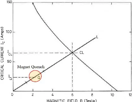
One of the most demanding aspects of all devices, is the reliability. In practical applications involving the use of superconducting wires such as magnets windings, the performances of these wires are always lower than those of tests carried out on short conductor samples. This effect, referred as coil degradation, consists in a magnet quench, i. e. any part of magnet goes from superconducting to the normal resistive state, at currents much lower than the critical current measured on a short sample, typically in the region Q of Fig. 1.11.

The problem is usually caused by a sudden rise of temperature in a wire region, due to different kinds of local disturbances (wire motion, flux jumping, AC losses, particle showers, etc [14, 79]), which causes the reduction of the superconductor critical current Ic. At the temperature value, referred as current sharing

temperature TCS, a sharing of the operating current IOp between the superconductor and the metallic

stabilizer starts, and an ohmic heating probably generates causing the quench. This process causes that the entire stored energy 1

2𝐿𝐼

2 _{∝ 𝐵}2 _{of the magnet is dissipated as heat.}

However, not only it is needed a certain density of energy to give life to a quench, but it is also important the energy impulse size. For triggering a quench, the dimension of the normal zone created volume (as showed in Fig. 1.12), must be greater than a certain volume referred as minimum propagation zone (MPZ). In determining the size of the MPZ it needs to consider the heat diffusion equation governing the temperature of a superconductor unit volume

Fig. 1.11: Short sample critical current Ic for a NbTi wire of 0.3 mm

29 𝐶(𝑇)𝜕𝑇

𝜕𝑡 = 𝛻 ∙ [𝜅(𝑇)𝛻𝑇] + 𝜌(𝑇)𝐽 2_{+ 𝑔}

𝑑+ 𝑔𝑐𝑜𝑜𝑙𝑖𝑛𝑔 (1. 41)

where the left-hand side represents the time rate of change of thermal energy density of the conductor, with C(T) as the heat capacity per unit volume of the composite conductor which consists of superconductor and normal-metal matrix [79]. In the right-hand side, the first term describes thermal conduction density into the composite superconductor element, where κ(T) is the thermal conductivity of the composite. The second term is Joule heating, with ρ as the normal state electrical resistivity, and J as the current density at operating current IOp(t), which can depend on time. Thermal disturbance is described

by gd, primarily magnetic and mechanical in origin, and the last term represents cooling. Assuming that

the conductor is characterized by a uniform and temperature-independent thermal conductivity κ, under time-independent and adiabatic conditions, with no dissipation other than Joule dissipation, i.e. 𝐶(𝑇)𝜕𝑇

𝜕𝑡 =

0 𝑔_𝑑= 0, 𝑔_{𝑐𝑜𝑜𝑙𝑖𝑛𝑔} = 0, in eq. (1.41), an expression for the length of the MPZ is derived:

𝑙_𝑀𝑃𝑍 ≈ √2𝜅(𝑇𝑐𝑠− 𝑇𝑂𝑝)

𝐽_𝑐2_𝜌 (1. 42)

where TOp is the operative temperature [14]. A normal zone which is longer than this will grow because

generation exceeds cooling; conversely a shorter zone will collapse, and full superconductivity will be recovered.

The smallest energy able to trigger a quench, referred as minimum quench energy MQE, is a key parameter in the evaluation of superconducting devices stability. In case of superconducting wires or tapes it is calculated from 𝑙_𝑀𝑃𝑍:

𝑀𝑄𝐸 ≈ 𝑙_𝑀𝑃𝑍𝑆_𝑇𝑜𝑡∫ 𝑐(𝑇)

𝑇𝐶𝑆

𝑇𝑂𝑝

𝑑𝑇 (1. 43)

Where STot is the cross section and c is the specific heat of conductor [14, 79].

Fig. 1.12: A thermal disturbance Qin

30 Superconductors have very small MPZs because they have very high resistivity ρ (in the normal state) and at the same time a very low thermal conductivity κ. Practical superconducting wires are therefore made in composite form, containing both superconductor and a normal conductor (usually copper or silver) [14]. Indeed, at low temperature, the resistivity of all pure metals decreases rapidly with temperature as the scattering of conduction electrons by lattice vibrations is reduced. At very low temperatures however, the resistivity reaches a constant value referred as residual resistivity ρres, very much lower electrical

resistivity than the resistivity ρ(273 K), determined by the impurity level and by other lattice defects. Moreover, their thermal conductivity is higher than superconductors. For example, the ratio 𝜅/𝜌 for the copper matrix is 7.5 x 106 _{higher than for the superconducting filaments of a NbTi wire [14].}

1.1.7 Normal zone propagation velocity

By designing any superconducting device, one wants to keep the MQE as large as possible for enhancing its stability. Nevertheless, this is not the only parameter that has to be kept under control. In a quench phenomenon, once a normal zone has started to grow, it will continue to expand at constant velocity referred under the combined actions of heat conduction and ohmic heating. This irreversible process is referred as normal zone propagation velocity (NZPV) and causes the entire stored energy 1

2𝐿𝐼

2_{of the}

magnet to be dissipated as heat. Therefore, the quench detection is a critical issue for superconducting magnets. The NZPV describes how fast the overheated zone propagates during a quench playing a key role in the protection strategies against quench-induced damages. In fact, the resistance of the normal zone and the corresponding resistive voltage are the vectors of the primary quench detection. Quench detection using voltage measurements is likely to be the fastest technical solution available [80].

The propagation of the perturbation along the conductor depends on the properties of the materials present in the winding. The NZPV can be evaluated following different approaches. The most practical way to evaluate the NZPV is to use the formulas that result from the solution of the heat equation describing the quench process [14, 79, 81]. The differential equation (1.41), describing the adiabatic quench process in a superconductor, with 𝑔𝑑= 0, 𝑔𝑐𝑜𝑜𝑙𝑖𝑛𝑔 = 0, becomes:

𝐶(𝑇)𝜕𝑇

𝜕𝑡 = 𝛻 ∙ [𝜅(𝑇)𝛻𝑇] + 𝑔𝑗(𝑇) (1. 44) Now, on the right-hand side, after the thermal conduction there is only the Joule heating [79]. In case of composite superconductor, the Joule heating is 𝑔_𝑗(𝑇) = 𝜌𝑚(𝑇)𝐽𝑚(𝑇)𝐽, where 𝜌𝑚 is the matrix electrical

resistivity, and Jm and J are the current density in the matrix and composite, respectively [82]. An

analytical expression for the NZPV in adiabatic conditions was derived assuming it as the velocity of a translating coordinate system representing the normal-superconducting boundary moving during a quench

31 [83]. In order to take into account the effects due to the current sharing between superconductor and metal matrix, the NZPV expression was further modified and the deduced formula is [82]:

𝑁𝑍𝑃𝑉 ≈ 𝐽 [ 1 𝜌_𝑛(𝑇_𝑡)𝜅_𝑛(𝑇_𝑡)(𝐶𝑛(𝑇𝑡) − 1 𝜅_𝑛(𝑇_𝑡) 𝑑𝜅_𝑛 𝑑𝑇|_{𝑇=𝑇𝑡}× ∫ 𝐶𝑆(𝑇)𝑑𝑇 𝑇𝑡 𝑇𝑂𝑝 ) ∫ 𝐶𝑆(𝑇)𝑑𝑇 𝑇𝑡 𝑇𝑂𝑝 ] −1 2⁄ (1. 45)

where the subscripts n and s indicate the normal and superconducting state, respectively, Tt is the transition

temperature, TOp is the operative temperature. The transition temperature Tt has been introduced in place

of the Tc in technical superconductors, in order to define an effective superconducting/normal boundary

during a quench, where the current sharing effects are important. In the case of LTS, Tt is generally

considered as the average value between the current sharing temperature and the critical temperature 𝑇𝑡 =

(𝑇_𝐶𝑆 + 𝑇_𝑐)/2. In HTS, Tt is more properly evaluated as the temperature at which the heat generation term

in eq. (1.44) assumes its average value in the current sharing temperature range:

𝑔𝑗(𝑇𝑡) = [∫ 𝑔𝑗(𝑇)𝑑𝑇 𝑇_𝑐

𝑇𝐶𝑆

] (𝑇⁄ 𝑐− 𝑇𝐶𝑆) (1. 46)

Neglecting the temperature dependence of the material properties, eq. (1.45) may be simplified to

𝑁𝑍𝑃𝑉 ≈ 𝐽 𝐶[ 𝜌𝜅 (𝑇𝑡− 𝑇𝑂𝑝) ] −1 2⁄ (1. 47)

Different approaches have been proposed to evaluate the NZPV by eq. (1.47) in LTS [14, 79]. However, due to the complications encountered in solving the more general eq. (1.45) these approaches are extended in the practice also to HTS.

32

1.2 Superconducting materials relevant for applications

After its discovery in Hg, the superconductivity was found in other metallic elements of the periodic table. Elemental superconductors are typically Low Temperature Superconductors (LTS) and their behaviour is well described in the BCS theory. Only three metals exhibit Type II superconductivity, namely Niobium, Vanadium and Technetium, but among them Nb is the only one relevant for applications. Indeed, Niobium is the one with the highest critical temperature (Tc = 9.2 K) [80]. Unfortunately, metallic superconductors

show very low critical magnetic fields, so their technological application was not promising because they did not support significant currents. When De Haas and co-workers began to investigate the behavior of superconducting alloys in magnetic field, they discovered that superconductivity could endure in significantly strong magnetic fields [84]. Today we know that it is possible thanks to the penetration of the magnetic field flux lines which are fixed through pinning forces in type II superconductors. Moreover, the introduction of defects enhances the magnetic field that the superconductor could tolerate before moving to the dissipative regime and the so-called hard superconductors are obtained.

Among the many metal alloys known today, Nb-based alloys have the best superconducting properties and are used in the manufacture of sensors, detectors, digital electronics and radio frequency devices [10, 85-87]. If the ratios between atomic species are well defined and there is a crystallographic order, we have intermetallic compounds. In general, superconducting intermetallic compounds achieve higher critical temperatures, the most important family of them being the A-15 type (with A3B formula). Within this family we found Nb3Ge (23 K), Nb3Ga (20 K), Nb3Sn (18 K) etc [88]. NbTi is another important Nb-based compound; it shows a critical temperature 𝑇_𝑐 ≈ 9.3 𝐾 and an upper critical field 𝐵_𝑐2~15 𝑇. The design of LTS materials for applications depends on several factors. For example, wires manufacture requires that they be used in the form of multifilament wires in a normal conductive matrix to increase the Jc, and to protect the device in case of quench (see wires section). NbTi multifilamentary wires with

a Cu composed matrix (NbTi/Cu) represent the largest application of LTS and superconductors in general. Other LTS compounds are used in the manufacture of superconducting devices, which are recommended in some applications because of their quantum nature and low-noise cryogenic operation environment. For example, hot-electron detectors are the best least noisy receivers in the radiation wave ranges of hundreds of GHz and of THz [89]. In particular, superconducting NbN-based hot-electron devices are very suitable for fast and ultrasensitive optical detection due to their recovery time, inductance and system-detecting efficiency [10] . Indeed, due to the superconducting energy gap 2Δ, that is the energy needed to create a quasiparticle and which is much lower than the semiconductors gap, a single crossing photon in a superconducting detector can give rise to an avalanche electron charge resulting in devices with energy resolution much higher than in a semiconductor detector [90].

33 The discovery of high-Tc superconductivity (HTS) in the cuprate compound La2-xBaxCuO4, with an onset

Tc of about 35 K, in 1986 by Bednorz and Müller [34], was followed by the discovery of copper-oxide

compounds with higher and higher transition temperature. This gave rise to great interest in these materials due to the prospect of room temperature superconductivity and to its practical applications. The only fact that they could work with the much cheaper cryogenic liquid Nitrogen has made this class of materials one of the most studied at all. However, early excitation was placated by the hard realities of these new materials due to several reasons. Indeed, these materials show a value of the coherence length very small compared to the unit cell size and a large number of degrees of freedom in the preparation of the compounds, which facilitate to have defects inside them.

The many HTS cuprate compounds discovered after 1986 share some main aspects [91]. First, the presence of CuO2 planes in their crystal structure (Fig. 1.13), which are responsible for the conduction phenomena. Second, the undoped cuprates are antiferromagnetic Mott insulators (i.e. a material in which conductivity vanishes as temperature tends to zero, while band theory would predict it to be metallic) and high-Tc superconductivity is created by doping them adding charge carriers. Being these charge carriers

holes or electrons, the cuprates are thus classified as either hole- or electron-doped. Third, conventional BCS theory cannot explain the behaviour exhibited by them and new models have been proposed, which are still under debate.

After the discovery of copper oxide superconductors and the success for their high critical temperature, the demand for new superconductors was still high because, in addition to an ever-increasing critical temperature, new technological requirements need higher critical fields.

The discovery of the iron-based superconductors (IBSCs) by the Tokyo Institute of Technology (TIT) group in 2008 had striking impact because superconductivity occurs in materials including iron (Fe) that

34 is a ferromagnetic element, which usually breaks Cooper pairs. In the last years, it has become clear that iron-based compounds are compatible with superconductivity under certain conditions. Moreover, there is a large variety in candidate materials and in pairing interaction, and many new superconductors have been discovered in this family in few years. Thus, it is still high the possibility of finding new superconductors with better physical characteristics.

There are many features of iron-based superconductors such as strength to impurities, a high upper critical field even close to the critical temperature, high magnetic field isotropy and an excellent grain boundary nature which are advantageous for wire application and allow IBSC wires to reach maximal critical currents under high magnetic field making them real competitors to cuprate high temperature superconductors. Moreover, in spite they have lower critical temperatures (the highest Tc for this class has

been reported to be about 55 K [92]) compared to those of HTSs, almost all iron-based superconductors are not affected by technical hurdles such as the metal-insulator transition or the d-wave symmetry of the order parameter, which can limit their applications [92-94].

The first iron-based superconductor prototype, discovered in 2006, was the compound LaFePO with a Tc

of 4 K [95]. Two years later was found the first high-temperature iron-based superconductor LaFeAsO which, after electron doping through substitution of O with F, reached the Tc at 26 K [41].

Until now, iron-based compounds have been distinguished in four main families of crystal structures identified by their atomic ratio (see Fig. 1.14):

 1111 family, with generic compound LnFeAsO, where Ln = lanthanides [96-97]; consisting of an alternate stack of FeAs (or in general FePn, with Pn = pnictogen) and LnO layers. The highest critical temperature Tc is about 55 K, that is the maximum ever reached by iron-based compounds

and was obtained substituting La with another lanthanide element, i.e. SmFeAs(O,F) and NdFeAsO [43].

Fig. 1.14: Crystal structures of representative iron-based superconductors, 1111, 122, 111, 11 type compounds [94].