The GreatSPN tool: recent enhancements

(1)

The GreatSPN Tool: Recent Enhancements

Soheib Baarir

∗

LIP6

Univ. Pierre et Marie Curie Paris

souheib.baarir@lip6.fr

M. Beccuti

† Dipartimento di Informatica Univ. del Piemonte Orientale

Alessandria

beccuti@mfn.unipmn.it

Davide Cerotti

Dipartimento di Informatica Univ. del Piemonte Orientale

Alessandria

davide.cerotti@mfn.unipmn.it

Massimiliano De Pierro

Dipartimento di Informatica Universit `a di Torino Torino

depierro@di.unito.it

Susanna Donatelli

Dipartimento di Informatica Universit `a di Torino Torino

susi@di.unito.it

Giuliana Franceschinis

Dipartimento di Informatica Univ. del Piemonte Orientale

Alessandria

giuliana@mfn.unipmn.it

ABSTRACT

GreatSPN is a tool that supports the design and the qual-itative and quantqual-itative analysis of Generalized Stochas-tic Petri Nets (GSPN) and of StochasStochas-tic Well-Formed Nets (SWN). The very first version of GreatSPN saw the light in the late eighties of last century: since then two main releases where developed and widely distributed to the re-search community: GreatSPN1.7 [12], and GreatSPN2.0 [7]. This paper reviews the main functionalities of GreatSPN2.0 and presents some recently added features that significantly enhance the efficacy of the tool.

1. INTRODUCTION

Generalized Stochastic Petri Nets (GSPN) [1] are Petri Nets that include timed and immediate transitions. Timed transitions have stochastic firing delays, while immediate transitions fire in zero time. Stochastic Well-Formed Nets [11] (SWN) are High Level Petri Nets (HLPN) where tokens can carry information and thus be distinguished (i.e. to-kens are “colored” as opposed to traditional “black” toto-kens), and the events are represented by transition instances which are parameterized on the basis of a number of “color vari-ables” associated with them. SWNs can have timed and immediate transitions, as in GSPNs. GreatSPN supports both GSPN and SWN-based performance evaluation either through discrete event simulation, or through the genera-tion of a Markov chain representing the model behavior in time (if transition firing times are exponentially distributed). One of the characterizing aspect of GreatSPN is the analysis (reachability graph and Markov chain generation) of SWNs, that is based on particularly efficient algorithms that exploit symmetries to limit the state space explosion problem.

GreatSPN was initially developed at the Computer Sci-ence Department of the University of Torino, Italy; currently also the Computer Science Department of the University of Piemonte Orientale in Alessandria, Italy, is actively con-tributing to its maintenance, development and distribution. The current distribution can be downloaded from the web page www.di.unito.it/∼greatspn: it runs on Linux,

So-∗This work has been done while S. Baarir was a temporary

researcher at the Universit`a del Piemonte Orientale

†M. Beccuti is working on a research contract for CNIT,

Research Unit of the Universit`a del Piemonte Orientale

laris and MacOS X1_{, and requires the Open Motif library}

for the graphical interface. It is also possible to download a VMware image including a Linux installation of the pack-age, that can be run on any platform for which a VMware virtual machine exists (e.g. Windows). Recently, the port-ing towards 64 bits architectures has started. The package is available free of charge for academic institutions and non profit organizations.

In the following we present GreatSPN2.0 basic functional-ities (Section 2) and some recently added features (that are also part of the current distribution): utilities for model con-struction and transformation in Section 3, and two modules for the efficient analysis of SWN models that are partially symmetric in Section 4.

A summary of the various interactions of GreatSPN with other Petri nets and non-Petri nets tools that have taken place over the years is presented in Section 5.

2. GREATSPN BASIC FEATURES

This section is an overview about the main features of the GreatSPN software distribution. Further details and technical aspects can be found in [7, 12, 17].

The GreatSPN software distribution is mainly composed of three groups of programs:

The Graphical User Interface: the GUI is developed above

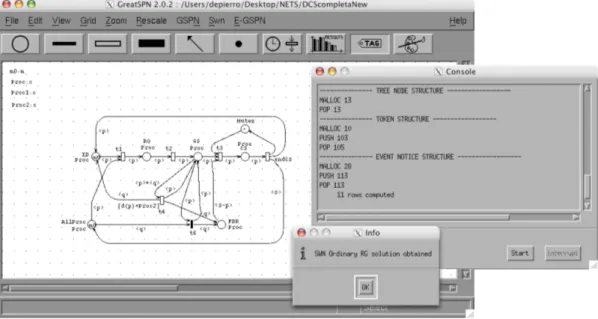
the Motif toolkit and besides the editing facilities allowing to draw a net and specify performance indexes, it allows to run the analysis modules (for structural properties, state space and performance indices computation) and show the results, to play the token game (GSPN only) and to perform an in-teractive simulation of timed and stochastic models (GSPN only). Figure 1 illustrates the GreatSPN’s GUI Main win-dow and the Console winwin-dow, which shows the output re-sults coming from the execution of an analysis module (in the figure it is shown the output of the SRG computation module applied to an example SWN). The GUI has limited support for the structuration of models into submodels: it only allows to place the net elements on different layers; compositional model construction is supported by an exter-nal utility (algebra) described later. It is possible to export models in eps or ps graphic formats (the model pictures 1_{For the moment only tested on version 10.4 and on PPC}

(2)

Figure 1: GreatSPN’s GUI: Main and Console windows

shown in this paper have been exported from GreatSPN).

The analysis modules: mainly implemented in C

program-ming language, these programs run in their own address-space, separately from the GUI, although a GUI’s Console window allows to call them from within the graphical en-vironment. The modules store the results of the analysis into files according to an internal format; several modules can cooperate (through intermediate result files) in order to compute a final result that requires several analysis steps;

Utilities: The GreatSPN distribution includes some

utili-ties: algebra, for models composition, a tool for graphical visualization of the reachability graph (see Section 3) and a tool implemented in Java, multisolve, which allows to run multiple experiments of a given analysis module in a batch of runs varying some model parameters, the output results are saved into a file suitable for the generation of graphs through the gnuplot program. In addition a number of “exporters” that translate the GreatSPN model description files into the formats accepted by other analysis and drawing tools are also available: see Section 5 for the details.

The analysis modules provided by the distribution can be classified into structural analysis modules, state-space anal-ysis modules, simulation modules and performance analanal-ysis modules based on the generation of a Markov chain (MC) and its numerical solution:

Structural analysis modules are available for GSPN mod-els only (although it is possible to apply them to unfolded SWN models). Among them there are: the P and T semi-flows computation module; the structural boundness and unbounded transition sequences computation modules; the structural traps and deadlocks computation modules. Sev-eral other kinds of net structural properties (whose results are useful to speed up other analysis algorithms) can be com-puted such as mutual exclusion, confusion, implicit places, causal connection, structural conflict, Extended Conflict Sets (ECS). A structural performance bound analyser is also avail-able, which requires lpsolve (lpsolve.sourceforge.net).

State-space analysis: for the uncolored formalisms an ef-ficient state space generation module is available, i.e. the Reachability Graph (RG) generator and the Tangible RG (TRG) generator that build the set of reachable markings and the transitions connecting them. Moreover a separate module computes several properties of the model state space (e.g. liveness, strongly connectedness, etc.). For the SWNs, both ordinary RG computation and more efficient Symbolic RG generation modules are available;

Simulation: event-driven simulation modules are available for both supported formalisms. The simulator allows to compute steady state performance indices through the batch means method. For SWNs the simulation can be performed either using ordinary markings and transitions or symbolic ones. Moreover, SWN ordinary simulation allows for timed transitions general firing time distributions. For GSPNs an interactive version cooperating with the GUI is also avail-able: it allows graphical animation of the model with move-ment of tokens, with step-by-step and automatic run, for-ward and backfor-ward time progression, real-time update of performance figures, arbitrary rescheduling of events. Markov chain generation and analysis modules: from the TRG or SRG a MC can be automatically generated; both transient (based on a randomization technique) and steady-state numerical analysis modules are then provided, to derive performance indices from the MC.

3. UTILITIES

One important choice in the development of GreatSPN has been the introduction of an HLPN formalism, SWNs, together with a suite of efficient algorithms for their analy-sis: this has greatly facilitated the construction of complex models, in particular those representing several entities with homogeneous behavior, and the analysis of qualitative and quantitative properties of the represented systems.

However the possibility of using an HLPN formalism is not enough when the model is more naturally specified in terms of interacting components. For this reason a net

(3)

composi-tion tool called algebra has been introduced, with the aim of supporting a compositional model construction approach. The algebra tool is a command line one, able to compose two subnets by superposition on (labelled) places, or tran-sitions or both. In this section we show algebra at work on a running example that will be used also throughout the paper for illustrating other GreatSPN tools and features.

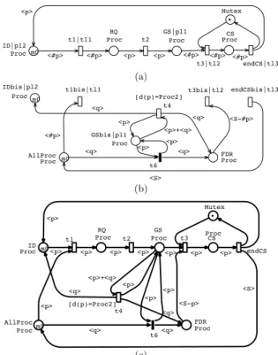
Let us consider a system where several users can require a resource to be used in mutual exclusion: the SWN model in Fig. 2(a) represents such situation; in this model “colors” (in

P roc) are used to distinguish the identity of token-customers

(in this section we assume P roc = {P roc1, P roc2}): the in-scriptions appearing on the arcs express the fact that the identity of the tokens is maintained while moving among places. Notice that at this abstract level of system represen-tation, keeping track of such identity is not actually needed: this over-specification may have quite a significant impact on the analysis complexity; the use of SWN-specific analy-sis tools (namely the Symbolic Reachability Graph – SRG – construction algorithm), recognizing that the customers be-have homogeneously and automatically abstracting out the irrelevant information, allows to alleviate the state space explosion problem. Let us now assume that the identities are necessary for the selection of the customer that has the right of getting exclusive use of the unique resource among the subset of customer who have issued a request (e.g. iden-tities correspond to customer priorities). The submodel in Fig. 2(b) represents a mechanism for the selection of the highest priority candidate for accessing the resource: it mim-ics a distributed selection process where pairs of customers compare their priorities, and the highest priority eliminates the lower priority one from the race. This process contin-ues until only one customer remains, which is the highest priority one that is hence assigned the resource. More in detail, place AllP roc contains the identities of the processes that are allowed to submit a request (initially the whole set P roc); place GSbis represents the requests that have reached the scheduler: when it is marked no new requests are accepted any longer (all tokens still in place AllP roc are moved to place F DR by immediate transition t6), and the selection process starts. Transition t4 performs the highest priority customer selection (the guard d(p) = P roc2 means that process p has highest priority: the request of process

q losing the race is discarded and sent back to place IDbis,

while p remains in GSbis); finally transition t3 represents the assignment of the resource to the race winner (it can fire only when all process identities except the winner are in place F DR, what is expressed by function < S − #p > on the arc). A new race can start only after the end of the resource usage by the current customer (firing of transition

endCS, which restores the whole set of customer identities

in place AllP roc through function < S > on the arc, thus making it possible the arrival of new requests).

The two submodels of Figs. 2(a) and 2(b) can be com-posed to form a complete model by superposition over la-beled places and transitions. In particular the places ID and GS, and the transitions t1, t3 and endCS in the first model, have an associated label (appearing next to the node name, separated by a | symbol) that allows to match them with the corresponding places and transitions in the sec-ond model, hence algebra can be employed to glue the two submodels. The result produced by algebra (after a light rearrangment of arcs) is shown in Fig. 2(c) (described in

Figure 2: SWN submodel of a mutually exclusive access to a shared resource (a), a submodel for selec-tion of the highest priority customer (b), and their composition (c)

tails in [6]). Much more complex composition situations are allowed, in particular several nodes in a submodel may con-tain the same label, moreover a node may be multi-labelled. Composition of n > 2 submodels can be achieved by a se-quence of successive compositions of model pairs. For more details on the use of algebra see [9, 17].

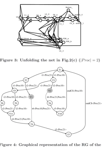
SWN analysis is supported by specific solvers. However any SWN can be automatically translated into an equiv-alent GSPN by means of an unfolding procedure. This allows to use analysis modules available for GSPNs only (e.g. the structural analysis ones) but can also be the first step towards the translation of a GSPN in other modeling languages for which analysis algorithms not supported by GreatSPN are available through other tools (e.g. this ap-proach has been used to export models to PRISM [10], as detailed in Section 5). The GreatSPN package embeds an unfolding tool that can transform an SWN into a GSPN. Fig. 3 illustrates the result of the unfolding of the net in Fig. 2(c) when the set of colors P roc (customer identities) has cardinality two: colored places and transitions are repli-cated and properly connected on the basis of their color domain. The model in Fig. 3 is the direct result of the automatic unfolding: some parameters allow to control the layout of the resulting model.

A new feature, recently introduced in GreatSPN, is the possibility to display graphically the (S)RG of a GSPN/SWN model. The (S)RG visualisation is performed in two steps and it is based on Graphviz (www.graphviz.org), an open source graph visualisation software, that includes several graph layout programs (e.g. dot, neato, twopi,. . . ).

(4)

ID_a CS_b CS_a Mutex_ ID_b RQ_b RQ_a GS_b AllProc_b FDR_b AllProc_a FDR_a GS_a t4_1 t4_3 t3_0 t3_1 endCS_0 endCS_1 t1_0 t1_1 t2_0 t2_1 t6_0 t6_1 t6_2 t6_3 _2

Figure 3: Unfolding the net in Fig.2(c) (|P roc| = 2)

T1 T2 t1<Proc21> T3 t1<Proc10> V1 t2<Proc21> T5 t1<Proc10> t1<Proc21> V2 t2<Proc10> T4 t6<Proc10,Proc21> T7 t3<Proc21> T8 t2<Proc10> T9 t2<Proc21> T6 t6<Proc21,Proc10> T10 t3<Proc10> endCS<Proc21> T11 t2<Proc21> t2<Proc10> endCS<Proc10> t4<Proc21,Proc10>

Figure 4: Graphical representation of the RG of the SWN model in Fig. 2(c)

is shown in Fig 4. This result is achieved in two steps: first the RG generation module for SWNs is run with a specific option so that an additional .dot result file is generated, this file is then parsed by the dot tool which generates the corresponding graph in a graphic format such as GIF, PNG, SVG or PostScript. The nodes in the graph are labeled with a short name: the complete marking description is stored in a separate textual file. Vanishing and tangible markings as well as immediate and timed transition firings are repre-sented in different colors (grey and black, respectively) to ease their identification.

4. NEW SOLUTION MODULES FOR SWN

The well-known state space explosion problem of com-plex systems can be contrasted in several ways, among them there are techniques based on the construction of a reduced graph equivalent to the RG w.r.t. some set of properties. In the context of (S)WNs, a symmetry based method can be applied, which builds the Symbolic Reachability Graph (SRG): each SRG node corresponds to a set of states lead-ing to an equivalent behavior. On the SRG one can study the reachability problem, temporal logic problems (when-ever the atomic propositions of the formula are symmetri-cal), but also the performance of the modeled system, solv-ing the lumped MC isomorphic to the SRG.

This approach has some limitations when the symmetric behavior of the modeled system has some exceptions: from an application point of view, it may happen that the (token) identities lead to asymmetric behaviors, e.g. in the context

of distributed algorithms identities can be used to break deadlock situations. Symmetry-based methods are not able to efficiently handle these partial symmetries, hence some strategy is needed to be able to efficiently treat these situ-ations. Two approaches have been developed to this pur-pose: the Extended SRG (ESRG) [6] and the Dynamic SRG (DSRG) [4], now distributed with GreatSPN [3].

The ESRG method: in this approach, an abstract state representation (called Symmetric Representation) is used which does not take the asymmetries into account, until some asymmetric transition becomes enabled, then a more refined marking representation (called eventuality) is used until the influence of the asymmetric firing is “absorbed” by a completely symmetric state.

In the SWN of Fig. 2(c) only transition t4 is asymmetric,

because of the guard d(p) = P roc2. Hence, the need to distinguish the elements of P roc2 from the other elements of color class P roc arises only when transition t4 is enabled.

The ESRG representation is based on extended symbolic

markings (ESM); each ESM is characterized by a symmet-ric representation (SR) not taking into account the

asym-metries, and possibly a set of eventualities, which refine the SR and take asymmetries into account: the eventualities are produced only when an asymmetrical transition is enabled in the ESM or when only a subset of the possible eventual-ities are reachable.

Whenever possible only SRs are maintained. In order to reduce the size of the ESRG it is also possible to discard the already generated eventualities of an ESM: this happens when the ESM becomes saturated (i.e. when all its eventual-ities have been reached) and all the asymmetric transitions fireable from them have been fired.

The DSRG method: in this approach, a system is mod-eled by use of two components: a completely symmetric SWN and a control automaton. In the symmetric SWN no references to particular identities are allowed, hence this SWN defines a superset of the behavior of the partially asymmetric system to be modeled.

The control automaton is an event-based automaton, used to reduce the symmetric SWN behavior to the actual one. This reduction is obtained by operating a synchronized prod-uct between the two components (in GreatSPN the automa-ton is specified in textual form through an additional file).

As an example, the system modeled by the SWN of Fig.2(c) would be modeled by a symmetric SWN, (without the guard

d(p) = P roc2), and a control automaton with one state, l,

and two arcs l_{−→l and l}¬t4 t4[p∈P roc2]_−→ _{l. Synchronizing the}

au-tomaton with the SWN any transition ti6= t4enabled in the

SWN are allowed to fire (synchronized with ¬t4) while only

those instances of t4 with p ∈ P roc2 are allowed.

The DSRG is as a directed graph where each node is com-posed of a symbolic marking and a state of the control au-tomaton. Based on the restrictions imposed by the control automaton each symbolic marking specifies its own degree of symmetry (represented by the so-called local partition, which partitions the identities keeping in the same subset those which in that state exhibit symmetric behavior). Con-trary to the traditional SRG method, that is based on the unique global partition of the identities taking into account all potential asymmetries of the model (statically defined at the net level), the DSRG partition is dynamically adjusted during its construction.

(5)

representations, the SR and the eventuality, in the DSRG many intermediate representations may exist, corresponding to abstraction levels in between the SR and the eventuality (and corresponding to sets of eventualities). One remarkable difference between the ESRG and the DSRG is that while the ESMs always represent disjoint subsets of eventualities, the DSRG nodes may have non null intersection.

The efficiency of the ESRG approach is measured by the number of SR (without eventualities) that are present in it. Since eventualities may be generated and then discarded when the ESM they belong to reaches saturation, this gen-erates a memory peak problem (which can be relevant if sat-uration is reached late in the ESRG computation).

Also, the derivation of a (lumped) MC from the ESRG is not straightforward: in fact the final structure does not always satisfy the (strong/exact) lumpability condition (as the SRG does). Hence an algorithm, to compute the coars-est Refined ESRG (RESRG) that satisfies the exact or the strong lumpability condition, must be derived. In [6], an ef-ficient algorithm, based on the Paige and Tarjan’s partition refinement algorithm, is proposed. Also this refinement al-gorithm may suffer from a memory peak problem: to satisfy the desired lumpability condition (exact or strong), the re-finement of some SRs into its eventualities may be required. The generated eventualities are kept in memory until the end of the computation. Hence the peak evolution depends on the number of SRs involved in such refinement. If there is a wide domino-effect then the peak could prevent the com-putation of the RESRG and the corresponding lumped MC. In the worst case the final RESRG is equal to the SRG.

By construction, the DSRG satisfies the exact lumpability condition. Hence, it does not need further refinement, and does not exhibit any memory peak problem. On the other hand, due to the non null intersection between its nodes, it may grow beyond the size of underlying ordinary RG.

A final remark is important: the type of performance mea-sure of interest may have an impact on the state space re-duction method that can be applied: the MC derived from the SRG satisfies both exact and strong lumpability, hence the probability of any individual ordinary marking can be derived from the probability of the symbolic markings. Also the DSRG method builds an aggregate MC satisfying the exact lumpability. The ESRG refinement step can be per-formed according to either the strong or the exact lumpabil-ity condition, however only in the latter case the probabillumpabil-ity of each ordinary marking can be computed.

To give a flavor of the space saving that can be achieved by exploiting the ESRG and DSRG methods, let us indicate some figures for the model of Fig. 2(c) for the case |P roc| = 8 (note that when |P roc| > 2 the guard of transition t4 must be adapted to check that the identity of p is greater than the identity of q) the SRG has 23.041 states, the ESRG has 74 SRs plus 5.281 final eventualities (and a peak of 5.796). The number of states of the RESRG w.r.t. strong lumpability is 74, however the number of refined states that are instanti-ated to achieve the final RESRG is 5.327; when refining the ESRG w.r.t. exact lumpability, the RESRG size is 547 with an intermediate peak of 6.343 states. Finally the DSRG size is 4.168 (in between the peak and the final RESRG size). In general, the degree of space saving can span several orders of magnitude, depending on the locality of the asymmetric behavior. Other figures illustrating the performance of the proposed methods can be found in [3, 4, 6].

5. INTERACTION WITH OTHER TOOLS

We distinguish two main types of interactions of Great-SPN with other tools: (1) export of net models to a receiving tool, in order to use analysis techniques available in the re-ceiving tool, (2) reuse of modules of GreatSPN (or part of them) by other tools.

Export to other tools. In its simplest form an export is a translation of the net description files (.net and .def) of GreatSPN onto the input files of the receiving tools, that might not necessarily be a Petri net tool.

For improved graphical manipulation of GSPN models, the gspn2tgif converter generates the .obj file format of TGIF (bourbon.usc.edu:8001/tgif); TGIF models are very convenient for inclusion in documents. An export to APNN (www4.cs.uni-dortmund.de/APNN-TOOLBOX), a GSPN tool, is also available (see [13]): if the GreatSPN net is split over layers, the translation maps layers on APNN partitions, so that the efficient Kronecker based Markovian solver of APNN can be used.

To allow GreatSPN users to check CSL [2] properties, two different translations are available. GSPN are trans-lated [10] into PRISM (www.prismmodelchecker.org): the PRISM language is based on variables and actions, and a model is usually a set of modules that interacts on actions. The translation produces a single module, mapping places onto variables of equal name. The user can then check CSL properties in which the atomic propositions are expressions over the variables (that is to say over the places). PRISM does not support priorities among transitions and therefore only SPNs can be successfully translated. SWN have instead to undergo an unfolding step, as described in Section 3. CSL model checking of SWN can also be realized using a different approach [10]: the SWN underlying MC is generated first, together with a set of atomic proposition that hold true in each state; the chain and the properties are produced in a format accepted by the MRMC tool (www.mrmc-tool.org), that allows to check CSL properties of the MC.

Reuse inside other tools. We consider two different types of reuse, depending on whether a full module, usually a solver with its input and output files, is called by another tool, or whether it is a function, or a portion of it, that has been reused, usually totally embedded into the receiv-ing tools code. Clearly the second option requires a deeper knowledge of the basic data structures of GreatSPN.

Examples of the first type are the tool PerfSWN [15] of the University of Savoie at Annecy for computing detailed performance indices of SWN nets based on the SRG analy-sis module and on SciLab(www.scilab.org), and the tool for computing bounds on Timed Petri Nets [8], that uses some of the modules for invariant computation and bounds com-putation of GreatSPN. Another extensive reuse of Great-SPN modules is what is done within the Draw-Net Mod-eling System [14], which supports a number of modMod-eling formalisms, including the possibility of creating new formal-ism based on existing ones, and possibly mixing them. In Draw-Net whenever GSPN or SWN nets are involved, the GreatSPN solvers have been reused: among all of them we mention the possibility to compose SWN models at a graph-ical level exploiting the algebra module of GreatSPN.

We do not know how many cases of code reuse of Great-SPN actually exist (the source code of the tool has been distributed since the very beginning to non profit organi-zations). Two significant ones are due to a collaboration

(6)

with the researchers of the LIP6 laboratory of the Univer-sity of Paris VI that have created and maintain CPN-AMI (move.lip6.fr/software/CPNAMI) and with the University of Savoie at Annecy. CPN-AMI includes a state space gener-ation and analysis of SWN based on a very efficient symbolic (decision-diagram like) data structure [16] which has mod-ified the GreatSPN functions for enabling and firing. The compSWN tool (an evolution of TenSWN [15]) developed at LISTIC, University of Savoie, uses modified SRG and as-sociated MC computation algorithms, in order to combine symmetry based method and Kronecker algebra based tech-niques to SWN models comprising several submodels com-bined through synchronous or asynchronous composition: this is particularly useful when modeling component-based architectures.

Finally the tool for the analysis of Markov Decision Well-formed Nets (MDWN) [5], integrated in Draw-Net, uses al-gebra to compose the non deterministic and probabilistic subnets of a MDWN, and a modified version of the SRG module to derive a Markov Decision Process from a MDWN.

6. CONCLUSIONS

The GreatSPN package is a mature software tool for per-formance evaluation of GSPN and SWN models: the latest developments have been oriented towards the integration of some utilities to ease the models construction, and the devel-opment and implementation of new efficient analysis mod-ules specifically oriented to the SWN high level formalism. The modular structure of the tool has favored the integra-tion of some of its modules within other frameworks. More-over several model translation tools have been developed to exploit other packages features. In several cases the SWN related functions have been reused in other tools: the pro-duction of a more accessible library to promote the reuse of such code is a medium term goal that the GreatSPN de-velopment team is pursuing within a collaboration with the MoVe group at LIP6, University of Paris VI.

7. REFERENCES

[1] M. Ajmone Marsan, G. Balbo, G. Conte, S. Donatelli, and G. Franceschinis. Modelling with Generalized

Stochastic Petri Nets. J. Wiley, 1995.

[2] A. Aziz, K. Sanwal, V. Singhal, and R. Brayton. Model-checking continuous time Markov chains. ACM

Trans. on Computational Logic, 1(1):162–170, 2000. [3] S. Baarir, M. Beccuti, and G. Franceschinis. New

solvers for asymmetric systems in GreatSPN. In Proc.

of the 5th Int. Conf. on Quantitative Evaluation of Systems (QEST08), pages 235–236, St. Malo, France,

Sep. 2008. IEEE CS Press.

[4] S. Baarir, C. Dutheillet, S. Haddad, and J.-M. Ili´e. On the Use of Exact Lumpability in Partially Symmetrical Well-formed Nets. In Proc. of the 2nd Int. Conf. on

Quantitative Evaluation of Systems (QEST05), pages

23–32, Torino, Italy, Sep. 2005. IEEE CS Press.

[5] M. Beccuti, D. Codetta-Raiteri, G. Franceschinis, and S. Haddad. A framework to design and solve Markov Decision Well-formed Net models. In Proc. of the 4th

Int. Conf. on Quantitative Evaluation of Systems (QEST07), pages 165–166, Edinburgh, UK, Sep. 2007.

IEEE CS Press.

[6] M. Beccuti, G. Franceschinis, S. Baarir, and J.-M. Ili´e. Efficient lumpability check in partially symmetric systems. In Proc. of the 3rd Int. Conf. on the

211–220, Riverside, CA, USA, Sep. 2006. IEEE CS Press.

[7] S. Bernardi, C. Bertoncello, S. Donatelli, G. Franceschinis, R. Gaeta, M. Gribaudo, and A. Horv´ath. GreatSPN in the New Millenium. In

Tools, 2001 Int. Multiconf. on Measurement, Modelling and Evaluation of Computer Communication Systems, pages 17–23, 2001.

TR760/2001 of the Universitat Dortmund (Germany).

[8] S. Bernardi and J. Campos. On Performance Bounds for Interval Time Petri Nets. In Proc. of the 1st

International Conference on Quantitative Evaluation of Systems (QEST04), pages 50–59, Enschede, The

Netherlands, Sep. 2004. IEEE CS Press.

[9] S. Bernardi, S. Donatelli, and A. Horv´ath.

Compositionality in the GreatSPN tool and its use to the modelling of industrial applications. Software

Tools for Technology Transfer, 3(4):417–430, 2001. [10] D. Cerotti, D. D’Aprile, S. Donatelli, and J. Sproston.

Verifying Stochastic Well-formed Nets with CSL Model-Checking Tools. In Proc. of the 6th Int. Conf.

on Application of Concurrency to System Design, ACSD06, pages 143–152, Turku, Finland, June 2006.

IEEE Computer Society.

[11] G. Chiola, C. Dutheillet, G. Franceschinis, and S. Haddad. Stochastic Well-Formed Coloured Nets for Symmetric Modelling Applications. IEEE Trans. on

Computers, 42(11):1343–1360, Nov. 1993. [12] G. Chiola, G. Franceschinis, R. Gaeta, and

M. Ribaudo. GreatSPN 1.7: Graphical Editor and Analyzer for Timed and Stochastic Petri Nets.

Performance Evaluation, special issue on Performance Modeling Tools, 24(1&2):47–68, Nov. 1995.

[13] S. Donatelli and P. Kemper. Integrating synchronization with priority into a Kronecker representation. Perform. Eval., 44(1-4):73–96, 2001.

[14] M. Gribaudo, D. Codetta-Raiteri, and G. Franceschinis. Draw-Net, a customizable multi-formalism, multi-solution tool for the

quantitative evaluation of systems. In Proc. of the 2nd

Int. Conf. on Quantitative Evaluation of Systems (QEST05), pages 256–257, Torino, Italy, Sep. 2005.

IEEE CS Press.

[15] J.-M. Ili´e, S. Baarir, M. Beccuti, C. Delamare, S. Donatelli, C. Dutheillet, G. Franceschinis,

R. Gaeta, and P. Moreaux. Extended SWN solvers in GreatSPN. In Proc. of the 1st Int. Conf. on

324–325, Enschede, The Netherlands, Sep. 2004. IEEE CS Press.

[16] Y. Thierry-Mieg, J.-M. Ili´e, and D. Poitrenaud. A Symbolic Symbolic State Space Representation. In

Proc. of the 24th Int. Conf on Formal Techniques for Networked and Distributed Systems, pages 276–291,

Madrid, Spain, Sep. 2004. LNCS 3235.

[17] Univ. di Torino and Univ. del Piemonte Orientale.

GreatSPN User’s Manual , 2008.Downloadable from www.di.unito.it/∼greatspn.