Regularizing deep networks with prior knowledge: A constraint-based approach

(1)

Contents lists available atScienceDirect

Knowledge-Based Systems

journal homepage:www.elsevier.com/locate/knosys

Regularizing deep networks with prior knowledge: A constraint-based

approach

Soumali Roychowdhury

a

_{, Michelangelo Diligenti}

b,∗

, Marco Gori

b,c a_{IMT Lucca, Italy}

b_{Department of Information Engineering and Mathematics, University of Siena, Italy} c_{Inria, CNRS, I3S, Université Côte d’Azur, Maasai, Côte d’Azur, France}

a r t i c l e i n f o Article history:

Received 2 December 2019

Received in revised form 21 March 2021 Accepted 24 March 2021

Available online 2 April 2021

Keywords:

Deep learning

Convolutional neural networks Image classification

Neuro symbolic methods First-order logic Learning from constraints

a b s t r a c t

Deep Learning architectures can develop feature representations and classification models in an inte-grated way during training. This joint learning process requires large networks with many parameters, and it is successful when a large amount of training data is available. Instead of making the learner develop its entire understanding of the world from scratch from the input examples, the injection of prior knowledge into the learner seems to be a principled way to reduce the amount of require training data, as the learner does not need to induce the rules from the data. This paper presents a general framework to integrate arbitrary prior knowledge into learning. The domain knowledge is provided as a collection of first-order logic (FOL) clauses, where each task to be learned corresponds to a predicate in the knowledge base. The logic statements are translated into a set of differentiable constraints, which can be integrated into the learning process to distill the knowledge into the network, or used during inference to enforce the consistency of the predictions with the prior knowledge. The experimental results have been carried out on multiple image datasets and show that the integration of the prior knowledge boosts the accuracy of several state-of-the-art deep architectures on image classification tasks.

1. Introduction

Deep Learning [1,2] has been a break-through for several classification and recognition problems. This success has been possible because of the availability of large amounts of training data, increased chip processing abilities, and the availability of well designed and general software environments. In particular, Convolutional Neural Networks (CNNs) [3] are very effective in complex pattern recognition tasks like image and video classifica-tion, and image segmentation. Deep neural networks have major disadvantages like their heavy dependency on a large amount of labeled data, which is required to develop powerful feature representations. Unsupervised data has been playing a minor role so far in the development of deep learning frameworks, and it has been only used to drive a proper initialization of the weights in a pre-training phase [4,5]. Unfortunately, it is difficult and labor intensive to manually annotate huge datasets in the era of big

The code (and data) in this article has been certified as Reproducible by Code Ocean: (https://codeocean.com/). More information on the Reproducibility Badge Initiative is available at https://www.elsevier.com/physical-sciences-and-engineering/computer-science/journals.

∗

Corresponding author.

E-mail addresses: soumali.roychowdhury@alumni.imtlucca.it

(S. Roychowdhury),diligmic@diism.unisi.it(M. Diligenti).

data. Therefore, to convert the empirical success of deep learning into a scalable solution, prior knowledge can be incorporated into the learners along with a smaller amount of labeled examples. Indeed, injecting prior knowledge in the learning framework can potentially allow to find better models by restricting the space where the learner should search its parameters. This mode of learning is more aligned to how the human brain seems to work, where high level knowledge and low level sensory inputs play a joint role in the development of human cognition abilities. Another limitation of deep architectures is that they mainly act as black-boxes from a human perspective. This makes their usage challenging in failure critical applications. The black-box behavior is both on the output side, which is hard to interpret, and on the input side which does not allow to encode human inten-tions [6]. This limitation can also be addressed by integrating logic rules into deep learners to encode human intentions and domain knowledge into the models to regulate the learning process.

This paper presents a constraint-based learning framework to inject prior knowledge into a deep learner. A fully differentiable generalization of First Order Logic (FOL) is used to express the prior knowledge about the learning task at hand. The clauses of the knowledge are converted into a set of differentiable con-straints, which are enforced during training together with the https://doi.org/10.1016/j.knosys.2021.106989

(2)

fitting of the supervised data. The framework is agnostic with re-spect to both the learner and injected prior knowledge, allowing large flexibility and a wide range of applications.

The experimental focus of this paper is on image classification, and shows the importance of the integration of prior knowledge for the improvement of many deep architectures on large-scale image classification datasets. This has been possible thanks to the definition of a constraint-based framework to integrate logic knowledge into any deep neural learner using a back-propagation schema, which can be transparently applied during the train and test phases, and the definition of an improved optimization pro-cedure that makes learning and inference feasible at the required scale.

The structure of the paper is the following: Section2presents some prior work in the literature about learning with constraints and image classification, Section 3presents the framework de-veloped in this paper to train classifiers respecting the available prior knowledge, and Section4presents the experimental results. Finally, Section5 draws some conclusions and discusses future work in this area.

2. Related works

The methodology presented in this paper finds its roots and inspiration in the work carried out by the Statistical Relational Learning (SRL) community, which has proposed various proba-bilistic logic frameworks to integrate logic inference and probabil-ity like Markov Logic Networks (MLN) [7], Hidden Markov Logic Networks [8], Probabilistic Soft Logic [9] and Problog [10].

However, bridging the gap between symbolic-based proba-bilistic reasoners, like the ones proposed by the SRL community, and sub-symbolic learning methods like neural networks is still an open research problem. For this reason, the integration of logic inference and learning has recently attracted a lot of interest. In the context of neural networks, hybrid approaches integrating logic reasoning and learning have been called neuro-symbolic approaches [11,12].

Semantic Based Regularization (SBR) [13,14] integrates a per-ception and a reasoning module in a hybrid learning system, where FOL clauses express the prior knowledge, relaxed into a continuous fuzzy representation integrated into the training objective. SBR was initially proposed for Kernel Machines as underlying learners but it can be easily extended to any other gradient-based learner. A preliminary application of SBR to image classification using neural networks was presented by Roychowd-hury et al. [15,16]. This paper significantly extends this previous work by defining a more general constraint-based approach to inject FOL into learning and with a much larger experimental evaluation.

Logic Tensor Networks (LTN) [17] is a neuro-symbolic ap-proach that employs the same translation of the prior knowledge used by SBR to inject prior knowledge into neural networks. Unlike the methodology proposed in this paper, LTNs are limited to the application of the knowledge at training time. As shown by the experimental results, it is of fundamental importance to employ the knowledge also during inference time, as there is no guarantee that the networks can distill non-trivial inference paths in their weights.

All the previously discussed neuro-symbolic approaches rely on the semantics of fuzzy logic to define the reasoning process. It is generally assumed to be equivalent to consider fuzzy logic reasoning from a syntactic or semantics point of view [18], as the syntactic manipulations and semantics of fuzzy logic are con-sistent for all sound and complete fuzzy theories [19]. However, syntactic approaches would have strong computational limita-tions, because of the explosion of possible manipulations with a

non-zero degree of truth. On the other hand, as shown in this paper, the semantics of fuzzy logic allow to cast the reason-ing process into a supervised learnreason-ing setup, which enables an efficient and parallel, although implicit, logic reasoning process.

Hu et al. [20] presets an iterative distillation method that transfers structured information of first-order logic rules into the weights of the neural networks. The framework is agnostic to the type of neural architecture that can be used. However, this distillation method only happens only at training time, with no generalization guarantees on the test data. The work from Xu et al. [21] introduces a semantic loss based on circuit compilation techniques [22] to bridge the gap between neural learning and logical constraints. Like the previous approach, this framework does not allow to apply the constraints at inference time and their experimental evaluation is only restricted to solve multi-class classification tasks.

Relational Neural Machines [23] integrate deep learners and MLN-like logic reasoning into a single graphical model, which co-trains the parameters of the symbolic and sub-symbolic layers. The methodology is very general and flexible like required for image classification tasks. However, RNMs but it could not scale up to problems of the size considered in this paper, since it would not be possible to compute the partition function for the fully grounded FOL knowledge.

The integration of logic programming with artificial neural networks has been applied to specific applications like breast cancer detection [24] and short text classification [25]. Semantic Sensitive Tensor Factorization (SSTF) [26] that incorporates the semantics expressed by an object vocabulary or taxonomy to tensor factorization. However, these methodologies build an ah-hoc integration of the domain knowledge and lack the generality and flexibility required to deal with generic domain knowledge in image classification tasks.

DeepProbLog [27] extends the popular ProbLog [10,28] frame-work with predicates that are approximated via neural netframe-works. DeepProbLog defines a distribution over logic programs.

Another recent line of research focuses on developing differen-tiable frameworks for logical reasoning. For example, Rocktäschel et al. [29][30] presents a theorem prover based on the Prolog backward chaining algorithm known as Neural Theorem Prover (NTP). NTP is differentiable with respect to symbol representa-tions in a knowledge base (KB) and, therefore, can learn any representations of predicates, constants and also first-order logic rules of predefined structure using back propagation. An NTP encodes relations as vectors using a frozen pre-selected func-tion. This can therefore be ineffective in modeling relations with complex and multifaceted nature. This line of research employs neural networks to embed the symbols into a continuous space where it is possible to establish a more flexible inference process. However, these methods cannot process low level pattern repre-sentations like the one representing images. TensorLog [31] refor-mulates logic reasoning as a tensor-based computation. However, TensorLog does not allow to jointly optimize the learners while performing inference and, therefore, it only allows to stack the learner and the reasoners into static and separate modules.

Finally, the integration of deep learning with Conditional Ran-dom Fields (CRFs) [32] is also an alternative approach to enforce some structure on the network output. This methodology has been proved to be quite successful on sequence labeling for natu-ral language processing tasks. Deep Structured Models [33,34] use a graphical model to bridge sensorial and semantic information. These models extend deep learners to learn complex feature representations considering the dependencies between the out-put random variables. The work of Chen et al. [34] proposes to build a structured model with arbitrary graphs along with deep features forming the potentials of a Markov Random Field (MRF).

(3)

They showed the effectiveness of these models in image tagging, whereas Lin et al. [33] applies deep structured models to semantic image segmentation. Both of these works focuses on imposing correlations or dependencies on the output random variables without any focus on logic reasoning like done in this work.

3. Learning from constraints and examples

This section presents a framework which can be used to inject complex prior knowledge and logical reasoning into deep learn-ers. Let us consider a multi-task learning problem where each task works on an input domain of labeled and unlabeled patterns. Tasks can be n-ary relations where the input is a tuple of patterns. Each input pattern is described by a tensor x

∈

Di

,

i

=

1

,

2

, . . .

,

where Diis an input domain. The set of patterns in the ith domain

is indicated as xi.

Let f

= {

f1

, . . . ,

fT

}

indicate a set of T multi-variate functions

such that fk is the function implementing the kth task. The kth

task is associated to the set of tuplesXk, which is a set of inputs

to the function built as Cartesian product of the input domains for the task. For example if the task is unaryXk

=

xd(k), with d(k)

being a function returning the index of the input domain of the task. For a binary task,Xkis the Cartesian product of the two input

domainsX_k

= {

xd1(k)

×

xd2(k)

}

, with d1(k)

,

d2(k) the indexes of the first and second input domains of the kth task, respectively.

The vector of values obtained by applying the function fkto

the set of patternsXkis indicated as fk(Xk), while f (X)

=

f1(X1)

∪

f2(X2)

∪

. . .

collects the groundings for all the functions. From the set of T functions that must be learned to solve the tasks, some are known a priori (evidence or given functions) whereas others are unknown functions (query or learn functions).

The T task functions have to meet a set of H constraints that can be expressed asΦh(f (X))

=

1, whereΦh

:

f (X)

→ [

0

,

1

]

describes the prior knowledge about the learning task. These functionals can express properties of a single function or can correlate the subset of functions to be learned. Learning can be helped by exploiting these correlations, which limit the param-eter space where good solutions can be found and, potentially, allows to learn with less examples. Finally, a set of examples Ek

⊂

Xkis provided as the supervised labeled data for the learning

task at hand. The weights of the tasks are indicated as w

=

{

w1

,

w2

, . . .}

with wkbeing the set of weights of the kth task.

The learning task is formulated as a constrained optimization problem where the overall cost function is composed by a term enforcing the fitting of the supervised data and a regularization term, under the constraints imposed by the prior knowledge: min w T

∑

k=1

β

k

∑

x∈Ek L(fk(x)

,

yk(x))

+

α

2 T

∑

k=1

∥

wk

∥

2 s

.

t

.

Φh

(

f (X)

) =

1

∀

h

=

1

, . . . ,

H

where

β

k is the strength of the fitting of the supervised data

(e.g. how much solutions should be penalized for not respecting it),

α

is a meta-parameter determining the strength of the weight regularization, Ek is the set of labeled data available for the kth

function, L(

· , ·

) is a loss function, yk(x) is the target output value

for the x pattern of task k.

A hard enforcement of the constraints is not often advis-able because of the limited computational power of the learning machine, and it would also conflict with the desired weight regularization. Therefore, a set of slack variables can be added to allow a soft-enforcement of the constraints:

min w T

∑

k=1

β

k

∑

x∈E_k L(fk(x)

,

yk(x))

+

α

2 T

∑

k=1

∥

wk

∥

2

+

H

∑

h=1

ξ

h s

.

t

.

1

−

Φ_h

(

f (X)

) = ξ

h

∀

h

=

1

, . . . ,

H Table 1

The operations performed by single units of an expression tree depending on the inputs x,y and the t-norm used.

op t-norm

Product Lukaseiwicz Weak-Lukaseiwicz

x∧y x·y max(0,x+y−1) min(x,y)

x∨y x+y−x·y min(1,x+y) min(1,x+y)

¬x 1−x 1−x 1−x

x⇒y min(1,y_x) min(1,1−x+y) min(1,1−x+y)

where

ξ = {ξ

1

, . . . , ξ

H

}

are the slack variables, such that

ξ

h

≥

0 as

Φh

(

f (X)

) ≤

1. The Lagrangian for previous constrained problem

translates to the following unconstrained min/max optimization problem: min w,ξ max λ T

∑

k=1

β

k

∑

x∈Ek L(fk(x)

,

yk(x))

+

α

2 T

∑

k=1

∥

wk

∥

2

+

H

∑

h=1

ξ

h

+

H

∑

h=1

λ

h

(

1

−

Φh

(

f (X)

) − ξ

h

)

where

λ = {λ

1

, . . . , λ

H

}

are the Lagrange multipliers for the

constraints.

The solution can be found at the saddle point, such that: ∂L ∂λh

=

1

−

Φ_h

(

f (X)

) − ξ

h

=

0. Substituting this condition back in the

Lagrangian, we get the following unconstrained problem:

min w T

∑

k=1

β

k

∑

x∈Ek L(fk(x)

,

yk(x))

+

α

2 T

∑

k=1

∥

wk

∥

2

+

H

∑

h=1

(

1

−

Φ_h

(

f (X)

))

(1) This constraint-based formulation allows to efficiently get ad-vantage of the often widely available unsupervised or partially supervised data as the constraints should be respected on all patterns. The following section shows how to integrate logic knowledge into the framework presented in this section. 3.1. Constraints and logic

First-order logic is a general and expressive mean to express the knowledge for most learning problems. FOL predicates are either fully known a priori for all possible groundings or are approximated via the functions that are learned, constants can be used to address single patterns and quantifiers can be used to express a behavior that should happen on all or a subset of patterns. Fuzzy FOL relaxes FOL knowledge into a real valued constraint by using t-norms [35] to compute the degree of sat-isfaction of the rule for a given grounding of the variables. The degree of satisfaction of a FOL formula is obtained by iteratively grounding the variables in a formula and combining the values using an aggregation operator, which represents the quantifier.

Grounded Expressions. T-norms [35] can be used to convert a propositional logic expression into a continuous and differ-entiable logical constraint. A t-norm fuzzy logic is defined by its t-norm t(a1

,

a2) that models the logical AND (

∧

). A t-norm expression behaves as classical Boolean logic when the variables assume crisp values: 0 (false) or 1 (true).

Given a variablea with continuous generalization a in

¯

[

0

,

1

]

, its negation

¬¯

a corresponds 1

−

a. The

∨

operator modeling logical OR is named t-conorm, and its semantic is also defined for each t-norm. Different t-norm fuzzy logic variants have been pro-posed in the literature.Table 1details the operations computed for the different logic operators for the most common t-norms. In particular, the Weak Lukasiewicz t-norm [36] has been recently

(4)

Fig. 1. Forward propagation of the values in the expression tree of a FOL formula

∀x[¬A(x)] ∨ [B(x)∧C (x)]for the single grounding when using the product t-norm. The output of the root node returns a value in[0,1]corresponding to the evaluation of the rule for the grounding.

proposed for translating logic inference into a differentiable opti-mization problem, since it defines a large class of clauses which are translated into convex functions. For this reason this t-norm has been used in the experimental section of this paper.

A grounded expression is a FOL rule, whose variables are assigned to specific constants. An expression tree is built for each considered grounded FOL rule, where the basic logic operations (

¬

, ∧, ∨

) are replaced by a unit computing the logic operation using a t-norm. The expression tree takes the output values of the grounded predicates as input, then it recursively computes the output values of all the nodes in the expression tree. The resulting value at the root evaluates the expression for the input grounded predicates. For example, consider the rule

∀

x

[¬

A(x)

] ∨

[

B(x)

∧

C (x)

]

where A

,

B

,

C are three predicates that must be approximated (via learning) by the unknown functions fA

,

fB

,

fC.

For any given grounding, the expression tree returns the output value: tE(f (x))

=

1

−

fA(x)

+

fA(x)

·

fB(x)

·

fC(x). Fig. 1 shows

the expression tree and the computation that is performed for the previous FOL rule grounded with x. As another example, lets consider the same rule but using the Weak Lukasiewicz t-norm as reported inTable 1, the expression tree returns the output value: tE(f (x))

=

min(1

,

1

−

fA(x)

+

min(fB(x)

,

fC(x))) for a given grounding

x.

Quantifiers. FOL typically uses two quantifiers to describe

over which constants a rule holds. The universal quantifier (

∀

) and the existential quantifier (

∃

) express the fact that a clause should hold true over all or at least one grounding. The degree of truth of a formula containing an expression E with a universally quantified variable xiis translated into the average of the t-norm

generalization tE(

·

), when grounding xi overXi. For the example

represented inFig. 1, the conversion of the clause would yield the following functional: Φ(f (X))

=

1

|

X

|

∑

x∈X tE

(

f (x)

) =

1

|

X

|

∑

x∈X 1

−

fA(x)

+

fA(x)

·

fB(x)

·

fC(x)

where

|

X

|

is the size of the sampleX. For the existential quanti-fier, the truth degree is instead defined as the maximum of the t-norm expression over the domain of the quantified variable. When multiple universally or existentially quantified variables are present, the conversion is recursively performed from the outer to the inner variables as already stated.

3.2. Back-propagation with logic constraints

Eq.(1)representing the cost function of the considered learn-ing task can be optimized via gradient descent, since theΦh(

·

) are

differentiable with respect of the function values and parameters.

Fig. 2. The back propagation of the error over the expression tree for the grounding x= ¯x of the FOL rule∀x[¬fA(x)] ∨ [fB(x)∧fC(x)]using the product

t-norm. The back propagated error reaches a leaf node and it is passed as error derivative for a further back propagation pass over the network implementing the function in the leaf node.

The derivative of the cost function with respect to the jth weight of the ith function

w

ijis computed as:

β

i

∑

x∈Ei

∂

L(fi(x)

,

yi(x))

∂

fi

· ∂

fi

∂w

ij

+

αw

_ij

−

∑

h

∂

Φh

∂

fi

· ∂

fi

∂w

ij

assuming that fi(

·

) is implemented by a neural network, _∂w∂fi_ij is

computed via back propagation over the network. On the other hand,∂Φh

∂fi can be computed via back propagation

over the expression tree. In particular, the forward propagation over the network is performed for each single grounding of the variables, then the satisfaction error E of the rule is computed based on the value at the root of the expression tree. The com-putation of the gradient with respect to the model weights is performed by using the chain rule backward over the expression tree: _∂∂_onE

=

_∂∂E

op(n)

·

∂op(n)

∂on where onis the output of the node n in

the expression tree, p(n) indicates the parent of node n in the tree. The root node is assumed to be the node 0 for which o0

=

tE

(

f (x)

)

and the derivative error at the root node is:_∂∂_oE 0

= −

∂Lc ∂Φk.

This establishes an efficient gradient computation schema over the expression tree, where the error of the considered constraint is back-propagated from the root to the leaves.Fig. 2shows the back propagation of the error for the example used across this paper

∀

x

[¬

fA(x)

] ∨ [

fB(x)

∧

fC(x)

]

. At the bottom of the expression

tree, the error reaches a leaf node, and it triggers a further back-propagation pass over the network implementing the function stored in that node.

3.3. Collective classification

Collective classification (CC) [37] is one of the basic Statistical Relational Learning (SRL) tasks. CC performs inference over a set of instances that are not independent, but correlated via a set of relationships. In this context, collective classification is used to refine the function output to be consistent with the available FOL knowledge. When the prior knowledge is employed during training time, the learning process encodes the knowledge into the parameters of the networks. However, there is no guarantee that the prior knowledge will be respected by the outputs on the test patterns, either because poor generalization or lack of predictive power of the selected architecture. Hence, the role of collective classification is to enforce the constraints also on the test data.

In particular, we indicate as fk(Xk′) the vector of values

ob-tained by evaluating the function fkover the input tuples of the

test setX_k′. The overall set of outputs can be collected into a single tensor: f (X′)

=

f1(X1′)

∪ · · · ∪

fT(XT′). The framework also admits

(5)

function fk. In this case, fk(Xk′) is assumed to be just filled with

default initial values equal to 0.5.

Collective classification can be formulated as a minimization problem that searches for the valuesf (

¯

X′

k)

= ¯

f1(X1′)

∪ · · · ∪ ¯

fT(X_T′) respecting the FOL formulas on the test data, while being close to the prior values established by the neural networks. This can be expressed as: min ¯ f (X ′) T

∑

k=1

β

k

∑

x∈X_k′ L(fk(x)

, ¯

fk(x)) s

.

t

.

Φh

(¯

f (X′)

) =

1

, ∀

h

=

1

, . . . ,

H

Adding the slack variables and imposing the conditions on the saddle point, the following unconstrained problem is obtained:

min ¯ f (X ′) T

∑

k=1

β

k

∑

, ¯

fk(x))

+

H

∑

h=1

(

1

−

Φ_h

(¯

f (X′)

))

₍₂₎

The learning task defined by Eq. (2) closely resembles the one defined by Eq.(1)with the difference that during collective clas-sification, the weights of the trained neural network are fixed, and no back propagation down to the network weights is performed. Furthermore, the network outputs provide a prior to collective classification that acts the same role of the supervised examples during training. It is worth noticing that, since the train and test data are expected to be drawn from the same distribution, the inference step performed via collective classification can soundly reuse the same

β

kvalues used during training. Therefore,

collec-tive classification has no effect on the overall complexity of the tuning process, as the number of meta-parameters remains the same.

3.4. Optimization

The cost functions defined by Eqs.(1)and(2)pose two issues. On one side, direct optimization is not easy because theΦh(

·

) can

be non-convex and with a large number of local minima [14]. Furthermore, the equations introduce many meta-parameters

β

k

,

k

=

1

, . . . ,

T , whose values must also be carefully selected.

Unfortunately, the number of functions can be very high in some applications like the ones presented in this paper. Therefore, an exhaustive grid search is not feasible. This section discusses some optimization heuristics used to alleviate these issues and to make training effective even in complex and large learning tasks.

Convexity and training phases. There is a large class of logic statements that have been shown to translate into con-vex constraints [38]. If restricting to a knowledge base with rules in this convex fragment, the resulting optimization prob-lem is not harder than training the networks to fit the super-vised data. For example, all universally quantified clauses us-ing definite clauses correspond to convex constraints. Therefore, the following optimization strategy has been employed in the experiments:

1. solve the optimization problem stated by Eq.(1)(or Eq.(2)

during CC) using only the convex constraints. This allows to efficiently find a good initial approximation of the best solution;

2. add the non-convex constraints and continue the optimiza-tion until convergence.

Meta-parameter validation. Collective classification corrects

the output of the networks to be consistent with the prior knowl-edge. The first term of Eq.(2)determines how much to penalize solutions deviating from the priors provided by the output of the neural networks. This cost may not be constant for all predicates, but it can depend on how reliable the output of a predicate is. In

particular, by relying on the accuracy measured over a validation set, it is possible to scale the penalty of the kth predicate as:

β

k

=

β ·

Acc(fk(Xkv))

,

where Acc(fk(Xkv)) is the accuracy of the kth task on the input

tuples X_kv for in the validation set, and

β

is a single meta-parameter to scale the overall cost. Therefore, the collective clas-sification task is reformulated as the following problem which has a single meta-parameter, which can be easily optimized by cross-validation: min ¯ f (X ′)

β

T

∑

k=1 Acc(fk(Xkv))

∑

, ¯

fk(x))

+ +

H

∑

h=1

(

1

−

Φh

(¯

f (X′)

))

(3) Using this heuristic, it is possible to make the information primar-ily flow from the predicates which are mostly correct to the less reliable one. This selection of the parameters helps the inference, allowing a simple and efficient meta-parameter tuning process. 3.5. Training and inference modes

The constraint-based framework defined in this paper is very flexible and can be used in different ways to improve the accuracy of a generic classifier:

•

Knowledge Distillation (KD): the FOL knowledge base is

used to force the underlying model to respect the rules. The training task expressed by Eq.(1)is used to inject the knowl-edge into the network weights. This distillation process is particularly useful in transductive [39], partially labeled or semi-supervised settings, where unsupervised data is avail-able during training. Indeed, the networks should respect the knowledge also on the unsupervised data. Therefore, enforcing the knowledge is a powerful and principled way to get advantage of the unsupervised data, which often plays a minor role in deep learning. For the image classification datasets considered in this paper, knowledge distillation can be performed by forcing the networks to respect the knowledge on all patterns (train, validation and test) by assuming a transductive context during training.

•

Collective Classification (CC): the trained CNN model is

considered as frozen with respect to the available knowl-edge. The knowledge is instead enforced during the infer-ence phase using the optimization problem defined by Eq.(2)

or(3).

•

Knowledge Distillation and Collective Classification: the

logical knowledge is enforced both during train and test by solving the optimization problem defined by Eqs. (1) and then using the output function values to instantiate a CC step using Eq. (2) or (3). As shown by the experimental results, enforcing the knowledge also at inference time is effective, even if the knowledge was already distilled in the network weights. Indeed, there is still no guarantee that the network output will respect the logic knowledge, either because of a lack of generalization, or the non-infinite approximation capabilities of the networks.

4. Experimental results

The experimental results have been performed on the CIFAR-10, CIFAR-100 and ImageNet image-classification benchmarks, studying the impact of the different training procedures on the

(6)

Table 2

Test set error rate (%) for the 10 final classes on CIFAR-10 and with collective classification over the network outputs for different deep architectures. CNN: raw network output, CC: collective classification over the network output, CC+O: collective classification using predicate specific meta-parameters KD+CC collective classification over the KD-enhanced networks, KD+CC+O collective classification over the KD-enhanced networks using predicate specific meta-parameters. Bold values mark a relative reduction of the error rate of 5% or more e.g. error<cnn_error×0.95.

Model CNN CC CC+O KD KD+CC KD+CC+O

NIN-50 8.81 8.71 8.66 8.20 8.12 8.07 Res-32 7.51 7.09 6.88 6.85 6.60 6.50 Res-110 6.61 5.96 5.54 5.52 5.13 4.91 Res-164 5.93 5.76 5.53 5.20 4.92 4.70 Res-1202 7.93 5.17 5.07 4.91 4.74 4.50 PRes-110 6.37 6.15 6.10 5.88 5.82 5.72 PRes-164 5.46 5.20 5.15 5.02 4.98 4.90 PRes-1202 6.85 6.05 6.01 5.80 5.72 5.60 APN-110,α =48 4.62 4.60 4.43 4.01 3.84 3.72 APN-164,α =84 3.96 3.95 3.66 3.10 2.81 2.70 APN-236,α =220 3.40 3.40 3.31 2.80 2.75 2.60 APN-272,α =200 3.31 3.30 3.22 2.70 2.61 2.50

final classification performances.1 Furthermore, several ablation studies have been performed to show how the prior knowledge can help in conditions where the training data is scarce. In all the reported experiments, we label the results using the following convention:

•

CNN: results obtained using a deep CNN network without any application of the prior knowledge. These entries re-fer to the results obtained by applying the networks as proposed in the corresponding original work.

•

CC: collective classification is performed over the CNN net-work outputs to enforce the consistency with respect to the prior knowledge. The collective classification step provides the actual considered output.

•

CC+O: like CC but the predicate-specific meta-parameters have been adjusted using the procedure defined in Eq.(3).

•

KD: results obtained by retraining the networks in a

trans-ductive context, where the knowledge is distilled into the network weights by enforcing its respect on all the avail-able data during training. The final classification is directly obtained from the network outputs.

•

KD+CC: starting from the network outputs obtained in the KD step, a collective classification step is triggered to fur-ther enforce the knowledge consistency on the predictions. The results are computed over the output of the collective classification step.

•

KD+CC+O: like KD+CC but the predicate-specific meta-parameters have been adjusted using the procedure defined in Eq.(3).

The Weak Lukaseiwicz t-norm has been used across all the reported experiments, because the initial tests showed that it was providing the most stable training and a final accuracy that was always comparable with the best obtained by the other t-norms. This confirms the theoretical results presented in [38].

4.1. CIFAR-10

The CIFAR-10 dataset [40]2 is a popular image classification benchmark, composed of 50,000 training and 10,000 test images.

1 _Code _and _instructions _on _how _to _replicate _the _experiments _can

be downloaded from https://sites.google.com/view/regularizingdeepnetworks/ home.

2 _{https://www.cs.toronto.edu/~kriz/cifar.html}

Table 3

Test set error rate (%) on CIFAR-10 for Resnet-32 with when varying the amount of training data. %Patterns refers to the percentage of data used in training. CNN, CC and CC+O refer to the baseline CNN with collective classification applied on the output of the networks with constant and variable regularizers, respectively. KD, KD+CC, KD+CC+O refer to the results obtained using the previous training setups but also applying knowledge distillation during training. Bold values mark a relative reduction of the error rate of 5% or more e.g. error<cnn_error×0.95.

Model %Patterns CNN CC CC+O KD KD+CC KD+CC+O

Res-32 10 26.62 25.51 25.10 25.04 24.65 24.13

Res-32 20 18.61 17.89 17.70 17.52 17.17 16.84

Res-32 50 12.14 11.99 11.90 11.83 11.46 11.09

Table 4

Sample of the prior knowledge used for the experiments on CIFAR-10. ∀x ANIMAL(x)∨TRANSPORT(x)

∀x TRANSPORT(x)⇒AIRPLANE(x)∨SHIP(x)∨ONROAD(x) ∀x ONROAD(x)⇒AUTOMOBILE(x)∨TRUCK(x)

∀x SHIP(x)⇒TRANSPORT(x) ∀x AUTOMOBILE(x)⇒ONROAD(x)

∀x ANIMAL(x)⇒BIRD(x)∨FROG(x)∨MAMMAL(x) ∀x BIRD(x)⇒ANIMAL(x)

∀x AIRPLANE(x)⇒TRANSPORT(x)

∀x MAMMAL(x)⇒CAT(x)∨DEER(x)∨DOG(x)∨HORSE(x) ∀x FLY(x)⇒BIRD(x)∨AIRPLANE(x)

∀x¬FLY(x)⇒CAT(x)∨DOG(x)∨HORSE(x)∨DEER(x)∨. . . ∀x CAT(x)⇒ ¬FLY(x) ∀x DEER(x)⇒ ¬FLY(x) ∀x TRUCK(x)⇒ ¬FLY(x) ∀x AUTOMOBILE(x)⇒ ¬FLY(x) ∀x BIRD(x)⇒FLY(x) ∀x AIRPLANE(x)⇒FLY(x)

Each pattern in the dataset is a 32

×

32 RGB natural image belonging to one of the 10 classes: AIRPLANE, AUTOMOBILE, BIRD, CAT, DEER, DOG, FROG, HORSE, SHIP, and TRUCK. Using WordNet3 and additional common knowledge, the 10 leaf classes have been recursively mapped into their hypernomy (a more general con-cept) obtaining a hierarchical taxonomical structure composed by 15 total classes. The taxonomy can be expressed via FOL by expressing that any pattern belonging to a leaf class belongs also to its parent class, for example with the rule

∀

x CAT(x)

⇒

MAMMAL(x). On the other hand, any pattern belonging to a high-level general class must also belong to one of the child classes in the hierarchy, for example a rule in this class is the following:

∀

x TRANSPORT(x)

⇒

AIRPLANE(x)

∨

SHIP(x)

∨

ONROAD(x). Finally, any pattern belonging to one leaf class cannot belong to a class corresponding to a different hypernomy like for the rule:

∀

x DEER(x)

⇒ ¬

FLY(x).Table 4shows a sample of the 33 rules that have been used for this task.

The knowledge base correlates the 10 output predicates with new intermediate ones derived from the hierarchical information of WordNet. These tasks are learned by the neural networks via additional output layers. During the distillation phase, the prior knowledge enforces the semantic consistency among the outputs of the trained classifiers. In the collective classification phase, this knowledge can be further enforced on the outputs when the network did not correctly generalize and failed to respect the rules.

Multiple state-of-the-art neural network architectures have been tested on this benchmark. In particular, Network in Network Models (NIN) [41], Residual Networks (Res) [42], Pre-activated (PRes) [43] and Pyramidal Residual Networks APN) [44] have been employed selecting the same setup reported in the corresponding original papers. Additionally, the same architectures have been trained with KD, and CC has been applied on their outputs.

(7)

Table 5

CIFAR-100 test set error rate (%) for the 100 fine classes for different archi-tectures. CNN: baseline network output, CC: collective classification over the network output, CC+O: collective classification using predicate specific meta-parameters, KD+CC: collective classification over the KD-enhanced networks, KD+CC+O: collective classification over the KD-enhanced networks using predi-cate specific meta-parameters. Bold values mark a relative reduction of the error rate of 10% e.g. error<cnn_error×0.9.

Model CNN CC CC+O KD KD+CC KD+CC+O

Res-32 29.5 27.4 27.0 25.8 25.2 24.8 Res-110 25.2 22.8 22.6 22.7 22.0 21.2 Res-164 25.2 22.8 22.6 22.3 21.9 20.5 PRes-164 24.3 22.6 21.2 21.5 21.0 19.8 APN-110,α =84 20.2 19.1 19.0 18.9 18.6 17.1 APN-110,α =270 18.3 17.2 17.1 16.5 16.1 15.4 APN-164,α =84 18.3 17.3 17.2 16.0 15.6 14.8 APN-164,α =270 17.0 16.0 15.9 15.8 15.4 14.2 APN-236,α =220 16.4 15.4 15.2 14.9 14.7 12.6 APN-272,α =200 16.4 15.3 15.0 14.4 14.1 12.0 MPN-110,α =27 18.8 17.7 17.3 16.7 16.2 14.4 WRes-16,γ =8 22.1 21.0 20.9 20.8 20.3 20.3 WRes-28,γ =10 20.5 19.7 19.2 19.0 18.8 17.1 WRes-40,γ =4 22.9 20.7 20.5 20.4 20.1 19.1 WRes-D-28,γ =10 20.0 19.1 19.0 18.6 18.1 18.2 WRes-D-RE-28,γ =10 17.7 15.6 15.5 15.0 14.9 14.8 WRes-D-C-28,γ =10 15.2 14.1 14.0 13.5 13.0 12.0 Table 6

Test set error rate (%) for the 10 final classes on CIFAR-100 for Resnet-32 when varying the amount of training data. CNN: baseline network output, CC: col-lective classification over the network output, KD+CC+O colcol-lective classification using predicate specific meta-parameters. KD, KD+CC, KD+CC+O refer to the results obtained using the previous training setups but also applying knowledge distillation during training. Bold values mark a relative reduction of the error rate of 10% e.g. error<cnn_error×0.9.

Model %Patterns CNN CC CC+O KD KD+CC KD+CC+O

Res-32 10 43.44 41.57 40.10 39.85 39.10 38.76

Res-32 20 39.27 38.18 37.40 36.90 36.40 36.01

Res-32 50 34.56 33.91 31.04 30.89 30.75 30.64

Table 7

Sample from the 200 rules used for CIFAR-100 experiments. ∀x REPTILES(x)⇒CROCODILE(x)∨DINOSAUR(x)∨. . . ∀x SMALL_MAMMALS(x)⇒HAMSTER(x)∨MOUSE(x)∨. . . ∀x TREES(x)⇒MAPLE_TREE(x)∨OAK_TREE(x)∨. . . ∀x BABY(x)⇒PEOPLE(x) ∀x BOY(x)⇒PEOPLE(x) ∀x GIRL(x)⇒PEOPLE(x) ∀x SNAKE(x)⇒REPTILES(x) ∀x TURTLE(x)⇒REPTILES(x) ∀x WILLOW_TREE(x)⇒TREE(x) ∀x LARGE_MAN-MADE_OUTDOOR_THINGS (x)⇒OUTDOOR(x) ∀x LARGE_NATURAL_OUTDOOR_SCENES(x)⇒OUTDOOR(x) ∀x MOTORCYCLE(x)⇒HAS_WHEELS(x) ∀x PICKUP_TRUCK(x)⇒HAS_WHEELS(x) ∀x TRAIN(x)⇒HAS_WHEELS(x)

The CC problems have been solved as reported by Eq. (2)with constant regularizers

β

k

=

β,

k

=

1

, . . . ,

T with

β

estimated

on a validation set composed of 5000 images held out from the train data. Then, the CC tasks have been solved using the per-predicate meta-parameters as reported by Eq.(3)according to the procedure described in Section 3.4. Collective classification has been performed for 300 iterations using a learning rate of 0.01.

Table 2 shows the classification error rates obtained on the test set for the considered NN models trained on CIFAR-10. The error is measured on the final 10 classes as standard for this benchmark.

Knowledge Distillation consistently provides an improvement in the generalization capabilities of all the considered architec-tures. Collective Classification is also very effective for all tested

models and, in particular, when combined with knowledge distil-lation further reduces the error rates. Finally, the meta-parameter validation schema proposed in Section 3.4 is also effective in finding better solutions. When these neural networks are trained from scratch, the training time is typically in the order of several hours depending on the size and the complexity of the networks. However, collective classification for 300 iterations takes only a few minutes to perform inference over the test patterns, which is a negligible overhead given the improvement in the classifi-cation metrics. Improvements are especially large for very deep networks like the 1202-layer Resnet and PreResnet which showed significant performance degradation in the original works due to over-fitting. Gains are smaller for the best state-of-the-art architectures but they are still remarkably present.

An ablation study was performed by reducing the data exam-ples during training by using only 10%, 20% and 50% of the train-ing data.Table 3shows the classification error rates for a Resnet-32 layered (Res-Resnet-32) deep neural network model. It emerges that the reduction of the error rate is larger when the training data is scarce. For example: when only 10% of the supervised examples are used, the error rate is reduced by 2.49% by applying collective classification to enforce the prior knowledge. On the other hand, the error rate is reduced 1.01% from its counterpart without using logical rules when using all the available supervised data. 4.2. CIFAR-100

The CIFAR-100 dataset is composed of 100 classes containing 600 images for each class [40].4 The images are split into a train and test set, such that there are 500 train and 100 test images per class, respectively. The 100 classes in this dataset are grouped into 20 super-classes determined using the WordNet5 hierarchy. Therefore, each image comes with a fine and coarse label, corresponding to class and super-class to which the pattern belongs, respectively. The prior knowledge used for this task is divided into two groups: the first group consists of 150 logic rules that correlates the fine classes with the coarse/super classes consisting of 100 fine predicates and 20 coarse predicates of the taxonomy. For example, the rule

∀

x BABY(x)

⇒

PEOPLE(x) belongs to this portion of knowledge expressing taxonomical information from WordNet. Five additional classes MAMMALS, HOUSEHOLD, OUTDOOR, TRANSPORT, HAS_WHEELS. have been added to de-fine a second group of knowledge rules to express additional handcrafted semantic information like whether an object occurs indoor or outdoor, whether it should have wheels, etc. For exam-ple, the rule

∀

x TRAIN(x)

⇒

HAS_WHEELS(x) belongs to this third class. The resulting knowledge base is composed by 200 rules, and a small sample of them is reported inTable 7.

Classification performances have been tested for different deep architectures: 32, 110, 164 layered Resnets (Res) [42], 164 layered Preactivated Resnets (Pres) [43], 110, 164, 200, 236 and 272 layered Pyramidal Resnets (APN) [44], 110-layer Multiplica-tive Pyramidal Resnets (MPN) [44], 16, 28 and 40 layered Wide Residual Networks (WRes) [45] with the widening factor of 4, 8 and 10. Regularization technique like random erasing and cut-out [46,47] have been applied as reported on the original paper for 28 layered Wide Residual Networks (WRed-D) [48] (widening factor of 10). All the deep CNN models are initialized from the same weight initialization and trained for 150 to 300 epochs (de-pending on the network size) with the additional classifier layers similar to the CIFAR-10 experiments. All the hyper-parameters and other data augmentation techniques have been employed as reported in the original works.

4 _{https://www.cs.toronto.edu/~kriz/cifar.html} 5 _{https://wordnet.princeton.edu}

(8)

Table 8

Subset of the knowledge base used for the ImageNet experiments. ∀x PERSON(x)∨FOOD(x)∨ARTEFACT(x)∨ANIMAL(x)∨ · · · ∀x ANIMAL(x)⇒AMPHIBIAN(x)∨REPTILE(x)∨FISH(x) . . . ∀x AMPHIBIAN(x)⇒ANIMAL(x)

∀x REPTILE(x)⇒ANIMAL(x)

∀x AMPHIBIAN(x)⇒BULLFROG(x)∨TREE_FROG(x)∨ · · · ∀x BULLFROG(x)⇒AMPHIBIAN(x)

∀x TREE_FROG(x)⇒AMPHIBIAN(x) ∀x TAILED_FROG(x)⇒AMPHIBIAN(x)

∀x REPTILE(x)⇒SNAKE(x)∨CROCODILIAN(x)∨ · · · ∀x SNAKE(x)⇒REPTILE(x)

∀x CROCODILIAN(x)⇒REPTILE(x) ∀x DINOSAUR(x)⇒REPTILE(x)

∀x SNAKE(x)⇒VIPER(x)∨SEASNAKE(x)∨ELAPID(x) . . . ∀x RATTLE_SNAKE(x)⇒VIPER(x)

∀x RELATIVE(x)⇒PERSON(x)

The classification accuracy on the test set for the final 100 classes is shown inTable 5. An ablation study is also performed on Resnet-32 using a variable percentage of supervised data points.

Table 6shows the effect of logical constraints when 10%, 20% and 50% of supervised examples are used for training the networks and then applying collective classification on the outputs. It is observed that the reduction of the error rate is more signifi-cant when the training data is scarce both when using fixed or predicate-specific meta-parameters.

4.3. ImageNet

ImageNet is a large and popular image database organized according to the WordNet hierarchy composed of 1000 classes6 and used by the ILSVRC challenges since 2010. In particular, the ILSVRC 2012 dataset was used for the reported experiments. This dataset has approximately 1.3 million training images, 50,000 validation images and 100,000 test images. Each image shows a single object and it is in an RGB and high resolution format. The images are typically resized and cropped to 224

×

224 pixels before being processed by the CNN architectures to limit the computational resources needed to process the dataset. Each object category also has several levels of hierarchy in the word sysnets, of which we considered the top-2 levels. For example: the category DOG corresponds to a path from the specific to more general categories as DOG

→

MAMMAL

→

ANIMAL. These semantic and hierarchical relationships are explored to enforce the logical constraints and establish semantic consistency among the outputs. The knowledge base correlates the 1000 output predicates with the ones that are additionally added through handcrafted rules or from the taxonomical structure of the sys-nets. The overall knowledge is formed by 3210 rules, andTable 8

shows a small sample of them.

Resnets [42] with 50, 101 and 152 layers, Pre-activated Resnets [43] with 152 and 200 layers and Additive Pyramid Resnets [44] with 200 layers are used to test the image clas-sification performance on ImageNet using this framework. The output layer with 1000 neurons corresponding to the 1000 leaf predicates has been paired with two additional output layers with 1600 and 5 neurons, corresponding to the intermediate and the most general predicates (super-classes) used in the knowledge, respectively. Since retraining the state-of-the-art networks from scratch for the ImageNet dataset requires a huge amount of com-putational power, the networks are retrained for only the output classification layers. For this reason, no KD has been performed for this task, but the reported results are based on CC applied on

6 _{https://http://image-net.org/challenges/LSVRC/}

Table 9

Test set top-1 error rate (%) for the 1000 leaf classes on ImageNet for different deep architectures. CNN refers to the baseline network, while CC, CC+O refer to the collective classification error rates with constant and predicate-specific meta-parameters, respectively. Bold values mark a relative reduction of the error rate of 5% or more e.g. error<cnn_error×0.95.

Model CNN CC CC+O Res-50 24.70 24.10 23.80 Res-101 23.60 23.10 22.90 Res-152 23.05 21.20 21.30 PRes-152 22.20 21.05 20.90 PRes-200 21.90 20.90 20.30 APN-200α =300 20.50 19.20 18.90 APN-200α =450 20.10 18.96 18.14 Table 10

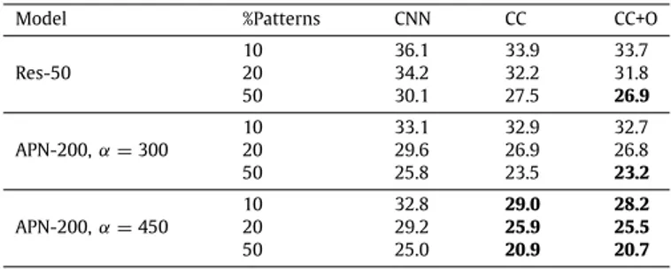
Collective classification error rates for 1000 final classes of ImageNet using a portion (%Patterns) of the training data and collective classification to enforce the semantic consistency of the outputs. CNN refers to the baseline network, while CC, CC+O refer to the collective classification error rates with constant and predicate-specific meta-parameters, respectively. Bold values mark a relative reduction of the error rate of 10% with respect to the baseline e.g. error <

cnn_error×0.9.

Model %Patterns CNN CC CC+O

Res-50 10 36.1 33.9 33.7 20 34.2 32.2 31.8 50 30.1 27.5 26.9 APN-200,α =300 10 33.1 32.9 32.7 20 29.6 26.9 26.8 50 25.8 23.5 23.2 APN-200,α =450 10 32.8 29.0 28.2 20 29.2 25.9 25.5 50 25.0 20.9 20.7

the network outputs as this adds a minimal overhead (less then 1%) compared to the network training time.

The error rates on the 1000 leaf classes for the test set are shown inTable 9for different CNN architectures. Collective clas-sification improves on top of the baseline (CNN) by approximately 0.6%–1.2% when using constant regularization parameters (CC) and by approximately 1%–2.0% with the per-predicate parameters (CC+O).

Table 10reports the results on the ImageNet test set when training the deep networks using a subset of the available su-pervised data. The results show that it is possible to use only 50% of the available supervisions in combination with the logical rules, and get a classification accuracy that is almost as high as using 100% of the supervisions but without employing the logic rules. This is an important outcome given the large computational cost in training a deep network on a large dataset like ImageNet. For example, the Additive Pyramid Resnet-200 with 1.3 million supervised data examples but no logic rules, has a classification error rate of 20.1%, whereas with only half of the supervised examples and using logical constraints, the error rate obtained by the same model in the CC+O train configuration is 20.7%. 4.4. Discussion

Knowledge distillation injects the prior knowledge into the model weights, showing that the networks are not always able to infer and generalize this information from the training data. Therefore, making the knowledge explicit and distilling it into the model improves the results in all tested configurations.

A similar effect at test time is due to collective classification, which employs the scores of the classes at all levels of the taxonomy to fix some of the classification errors. This also shows that the neural networks are not able to always generalize the

(9)

high level domain knowledge from the data, and enforcing it at inference time is of very important to maximize the final accu-racy. For this reason, neuro-symbolic methods that are limiting their application at training time are at a disadvantage in the considered task.

It is interesting to notice that there is a significant and posi-tive cumulaposi-tive effect introduced by employing both knowledge distillation and collective classification. Whereas KD is powerful, there are no generalization guarantees for how the knowledge is used on the test data. Better generalization of the domain knowledge can be obtained by limiting the network computa-tional power (e.g. smaller and simpler models), but this makes harder for the network to learn the knowledge in the first place, as the computational power is already heavily used to process the images. On the other hand, a complex model could learn the rules but it is likely to overfit them and not generalize them correctly to the test data. For this reason, the experiments show that the co-application of knowledge distillation during training and collective classification in test helps generalization and provides a further boost of the accuracy metric for most of the tested models. Finally, fine tuning the parameters over the single predicates gives extra flexibility in optimizing the trade off between enforc-ing the logic knowledge and fittenforc-ing the supervised data.

5. Conclusions

This paper presents a framework to integrate general prior knowledge into a deep learner, allowing to distill the knowl-edge into the model weights during training and to enforce the consistency of the predictions at the test time. Some heuristics have been presented to make the underlying inference process tractable and effective on large scale datasets. The experimental evaluation shows how the integration of semantic knowledge into learning improves the accuracy of several state-of-the-art architectures on image classification tasks. Future work will focus on a more scalable estimation of the rule strengths and the automatic learning of the prior knowledge, which should be used alongside to any available human knowledge.

CRediT authorship contribution statement

Soumali Roychowdhury: Conceptualization, Methodology,

Software, Data curation, Experiments, Validation. Michelangelo

Diligenti: Conceptualization, Methodology, Writing, Software. Marco Gori: Supervision, Conceptualization.

Declaration of competing interest

The authors declare that they have no known competing finan-cial interests or personal relationships that could have appeared to influence the work reported in this paper.

Acknowledgments

This project has received funding from the European Union’s Horizon 2020 research and innovation program under grant agreement No 825619.

References

[1] Y. LeCun, Y. Bengio, G. Hinton, Deep learning, Nature 521 (7553) (2015) 436.

[2] Y. Bengio, Learning deep architectures for AI, Found. Trends Mach. Learn. 2 (1) (2009) 1–127.

[3] L. Deng, D. Yu, J. Platt, Scalable stacking and learning for building deep architectures, in: Acoustics, Speech and Signal Processing (ICASSP), 2012 IEEE International Conference on, IEEE, 2012, pp. 2133–2136.

[4] D. Erhan, Y. Bengio, A. Courville, P.-A. Manzagol, P. Vincent, S. Bengio, Why does unsupervised pre-training help deep learning? J. Mach. Learn. Res. 11 (Feb) (2010) 625–660.

[5] Y. Bengio, P. Lamblin, D. Popovici, H. Larochelle, et al., Greedy layer-wise training of deep networks, Adv. Neural Inf. Process. Syst. 19 (2007) 153.

[6] A. Nguyen, J. Yosinski, J. Clune, Deep neural networks are easily fooled: High confidence predictions for unrecognizable images, in: Proceedings of the IEEE Conference on Computer Vision and Pattern Recognition, 2015, pp. 427–436.

[7] M. Richardson, P. Domingos, Markov logic networks, Mach. Learn. 62 (1–2) (2006) 107–136.

[8] J. Wang, P. Domingos, Hybrid Markov logic networks, in: Proceedings of the 23-Rd AAAI Conference on Artificial Intelligence, 2008, pp. 1106–1111. [9] S.H. Bach, M. Broecheler, B. Huang, L. Getoor, Hinge-loss Markov random fields and probabilistic soft logic, J. Mach. Learn. Res. 18 (109) (2017) 1–67.

[10] L.D. Raedt, A. Kimmig, H. Toivonen, ProbLog: A probabilistic prolog and its application in link discovery, in: Proceedings of the International Joint Conference on Artificial Intelligence (IJCAI), 2007, pp. 2462–2467. [11] L. De Raedt, R. Manhaeve, S. Dumancic, T. Demeester, A. Kimmig,

Neuro-symbolic= neural+ logical+ probabilistic, in: NeSy’19@ IJCAI, the 14th International Workshop on Neural-Symbolic Learning and Reasoning, 2019. [12] A.d. Garcez, M. Gori, L.C. Lamb, L. Serafini, M. Spranger, S.N. Tran, Neural-symbolic computing: An effective methodology for principled integration of machine learning and reasoning, 2019, arXiv preprintarXiv:1905.06088. [13] M. Diligenti, M. Gori, M. Maggini, L. Rigutini, Bridging logic and kernel

machines, Mach. Learn. 86 (1) (2012) 57–88.

[14] M. Diligenti, M. Gori, C. Sacca, Semantic-based regularization for learning and inference, Artificial Intelligence 244 (2017) 143–165.

[15] M. Diligenti, S. Roychowdhury, M. Gori, Integrating prior knowledge into deep learning, in: 2017 16th IEEE International Conference on Machine Learning and Applications (ICMLA), IEEE, 2017, pp. 920–923.

[16] S. Roychowdhury, M. Diligenti, M. Gori, Image classification using deep learning and prior knowledge, in: Proceedings Third International Workshop on Declarative Learning Based Programming (DeLBP 2018), 2018.

[17] L. Serafini, I. Donadello, A.S. d’Avila Garcez, Learning and reasoning in logic tensor networks: theory and application to semantic image interpretation, in: Proceedings of the Symposium on Applied Computing, SAC 2017, Marrakech, Morocco, April 3-7, 2017, 2017, pp. 125–130.

[18] P. Hajek, The Metamathematics of Fuzzy Logic, Kluwer, 1998.

[19] V. Novák, On the syntactico-semantical completeness of first-order fuzzy logic. II. Main results, Kybernetika 26 (2) (1990) 134–154.

[20] Z. Hu, X. Ma, Z. Liu, E. Hovy, E. Xing, Harnessing deep neural networks with logic rules, in: Proceedings of the 54th Annual Meeting of the Association for Computational Linguistics, 2016, pp. 2410–2420.

[21] J. Xu, Z. Zhang, T. Friedman, Y. Liang, G. Van den Broeck, A Semantic loss function for deep learning with symbolic knowledge, in: J. Dy, A. Krause (Eds.g), Proceedings of the 35th International Conference on Machine Learning, vol. 80, 2018, pp. 5502–5511.

[22] A. Darwiche, SDD: A new canonical representation of propositional knowl-edge bases, in: Proceedings of the International Joint Conference on Artificial Intelligence (IJCAI), 2011.

[23] G. Marra, F. Giannini, M. Diligenti, M. Maggini, G. Marco, Reational neural machines, in: Proceedings of the European Conference on Artificial Intelligence (ECAI), 2020.

[24] J. Neves, T. Guimarães, S. Gomes, H. Vicente, M. Santos, J. Neves, J. Machado, P. Novais, Logic programming and artificial neural networks in breast cancer detection, in: I. Rojas, G. Joya, A. Catala (Eds.), Advances in Computational Intelligence, Springer International Publishing, Cham, 2015, pp. 211–224.

[25] J. Wang, Z. Wang, D. Zhang, J. Yan, Combining knowledge with deep convolutional neural networks for short text classification, in: Proceedings of the International Joint Conference on Artificial Intelligence (IJCAI), 2017, pp. 2915–2921.

[26] M. Nakatsuji, Semantic sensitive simultaneous tensor factorization, in: P. Groth, E. Simperl, A. Gray, M. Sabou, M. Krötzsch, F. Lecue, F. Flöck, Y. Gil (Eds.), The Semantic Web – ISWC 2016, Springer International Publishing, Cham, 2016, pp. 411–427.

[27] R. Manhaeve, S. Dumancic, A. Kimmig, T. Demeester, L. De Raedt, Deep-problog: Neural probabilistic logic programming, in: Advances in Neural Information Processing Systems, 2018, pp. 3749–3759.

[28] L.D. Raedt, P. Frasconi, K. Kersting, S.M. (Eds), Probabilistic Inductive Logic Programming, Vol. 4911, in: Lecture Notes in Artificial Intelligence, Springer, 2008.

[29] T. Rocktäschel, S. Riedel, End-to-end differentiable proving, in: I. Guyon, U.V. Luxburg, S. Bengio, H. Wallach, R. Fergus, S. Vishwanathan, R. Garnett (Eds.), Advances in Neural Information Processing Systems 30, Curran Associates, Inc., 2017, pp. 3788–3800.

[30] P. Minervini, M. Bosnjak, T. Rocktäschel, S. Riedel, Towards neural theorem proving at scale, 2018, arXiv preprintarXiv:1807.08204.

(10)

[31] W. Cohen, Y. Fan, K.R. Mazaitis, Tensorlog: Deep learning meets probabilistic databases, J. Artificial Intelligence Res. 1 (2018) 1–15.

[32] X. Ma, E. Hovy, End-to-end sequence labeling via bi-directional LSTM-CNNs-CRF, in: Proceedings of the 54th Annual Meeting of the Association for Computational Linguistics, Association for Computational Linguistics, Berlin, Germany, 2016, pp. 1064–1074.

[33] G. Lin, C. Shen, A. Van Den Hengel, I. Reid, Efficient piecewise training of deep structured models for semantic segmentation, in: Proceedings of the IEEE Conference on Computer Vision and Pattern Recognition, 2016, pp. 3194–3203.

[34] L.-C. Chen, A. Schwing, A. Yuille, R. Urtasun, Learning deep structured models, in: International Conference on Machine Learning, 2015, pp. 1785–1794.

[35] E. Klement, R. Mesiar, E. Pap, Triangular Norms, Kluwer Academic Publisher, 2000.

[36] F. Giannini, M. Diligenti, M. Gori, M. Maggini, On a convex logic fragment for learning and reasoning, IEEE Trans. Fuzzy Syst. (2018).

[37] P. Sen, G. Namata, M. Bilgic, L. Getoor, B. Galligher, T. Eliassi-Rad, Collective classification in network data, AI Mag. 29 (3) (2008) 93.

[38] F. Giannini, M. Diligenti, M. Gori, M. Maggini, Learning Lukasiewicz logic fragments by quadratic programming, in: Proceedings of the European Conference on Machine Learning (ECML), 2017.

[39] V. Vapnik, The Nature of Statistical Learning Theory, second ed., Springer Verlag, 2000.

[40] A. Krizhevsky, G. Hinton, Learning Multiple Layers of Features from Tiny Images, Tech. rep., University of Toronto, 2009.

[41] M. Lin, Q. Chen, S. Yan, Network in network, 2013, arXiv preprintarXiv: 1312.4400.

[42] H. Kaiming, Z. Xiangyu, R. Shaoqing, S. Jian, Deep residual learning for image recognition, 2015, arXiv preprintarXiv:1512.03385.

[43] K. He, X. Zhang, S. Ren, J. Sun, Identity mappings in deep residual networks, in: European Conference on Computer Vision, Springer, 2016, pp. 630–645.

[44] D. Han, J. Kim, J. Kim, Deep pyramidal residual networks, in: Computer Vision and Pattern Recognition (CVPR), 2017 IEEE Conference on, IEEE, 2017, pp. 6307–6315.

[45] S. Zagoruyko, N. Komodakis, Wide residual networks, in: E.R.H. Richard C. Wilson, W.A.P. Smith (Eds.), Proceedings of the British Machine Vision Conference (BMVC), BMVA Press, 2016, pp. 87.1–87.12.

[46] T. DeVries, G.W. Taylor, Improved regularization of convolutional neural networks with cutout, 2017, arXiv preprintarXiv:1708.04552.

[47] W.-Z. Dai, Q.-L. Xu, Y. Yu, Z.-H. Zhou, Tunneling neural perception and logic reasoning through abductive learning, 2018, arXiv preprint arXiv: 1802.01173.

[48] Z. Wu, C. Shen, A. Van Den Hengel, Wider or deeper: Revisiting the resnet model for visual recognition, Pattern Recognit. 90 (2019) 119–133.