ANALYSIS OF DIFFERENT VISUAL STRATEGIES OF 'ISOLATED VEHICLE' AND 'DISTURBED VEHICLE'

(1)

ANALYSIS OF DIFFERENT VISUAL STRATEGIES OF ‘ISOLATED VEHICLE’

AND ‘DISTURBED VEHICLE’

Nicola BONGIORNO, Gaetano BOSURGI, Orazio PELLEGRINO, Giuseppe SOLLAZZO* Dept of Engineering, University of Messina, Italy

Received 4 August 2016; revised 1 December 2016; accepted 4 January 2017; published online 4 September 2017

Abstract. This paper analyses the driver’ visual behaviour in the different conditions of ‘isolated vehicle’ and ‘disturbed

vehicle’. If the meaning of the former is clear, the latter condition considers the influence on the driving behaviour of various objects that could be encountered along the road. These can be classified in static (signage, stationary vehicles at the roadside, etc.) and dynamic objects (cars, motorcycles, bicycles). The aim of this paper is to propose a proper analysis regarding the driver’s visual behaviour. In particular, the authors examined the quality of the visually informa-tion acquired from the entire road environment, useful for detecting any critical safety condiinforma-tion. In order to guaran-tee a deep examination of the various possible behaviours, the authors combined the several test outcomes with other variables related to the road geometry and with the dynamic variables involved while driving. The results of this study are very interesting. As expected, they obviously confirmed better performances for the ‘isolated vehicle’ in a rural two-lane road with different traffic flows. Moreover, analysing the various scenarios in the disturbed condition, the proposed indices allow the authors to quantitatively describe the different influence on the visual field and effects on the visual behaviour, favouring critical analysis of the road characteristics. Potential applications of these results may contribute to improve the choice of the best maintenance strategies for a road, to select the optimal signage location, to define forecasting models for the driving behaviour and to develop useful instruments for intelligent transportation systems.

Keywords: visual behaviour, road safety, isolated vehicle, disturbed vehicle, driving behaviour, traffic.

Notations

Variables and functions:

FT – curve Fixation along Tangent: time range be-tween the starting of the inner edge fixation and the beginning point of the curve (i.e. the tangent point between the previous tangent section and the curve);

FC – curve Fixation along Curve: the time range be-tween the beginning point of the curve and the end of the inner edge fixation;

NFC – No curve Fixation along Curve: the time range between the end of the inner edge fixation and the end point of the curve (i.e. the tangent point between the curve and the following tangent sec-tion) of the second variable;

TF – Total curve Fixation: the whole time range taken for the fixation of the curve inner edge (TF = FT + FC).

Abbreviations:

GPS – Global Positioning System; OBD – On Board Diagnostic; R – curve radius [m]. Introduction

The behaviour of a user driving an ‘isolated vehicle’ is chosen as a reference for almost all the road standards, and several safety checks have been defined in compli-ance with this condition. Anyway, many researchers in all the world have already understood that a vehicle dis-turbed by external causes (traffic, weather conditions, human activities at the roadside, activities inside the ve-hicle, etc.) could be conditioned so as to affect the ma-noeuvre accuracy. However, the choice was to propose the easiest solution, considering some specific reasons widely acceptable at that time:

– traffic volumes were really low;

– vehicle speeds were sufficiently moderate; *Corresponding author. E-mail: gsollazzo@unime.it

This is an Open Access article distributed under the terms of the Creative Commons Attribution License (http://creativecommons.org/licenses/by/4.0/), which permits unrestricted use, distribution, and reproduction in any medium, provided the original author and source are credited.

(2)

– there were not the computational potentialities of the modern computers;

– there were not specific instruments for monitor-ing objectively the men’s behaviour while drivmonitor-ing. During the recent decades, the increase in the ve-hicle speeds and in the traffic volumes, as well as in the activities inside the car (due to the introduction of board computers, GPS navigation systems, mobile phones, etc.), has essentially changed the situation. In detail, the accident analyses have evidenced how the hypothesis of ‘isolated vehicle’ could no longer be accepted as a standard reference for the road design, especially in very complex environmental scenarios. At the same time, the continuous development of instruments such video cam-eras, sensors, and GPS has produced smaller and cheap-er devices for monitoring the driving behaviour and, in particular, the visual activity. The vision mechanism is properly considered as the main acquisition channel for obtaining the major relevant information coming from the road context. Then, the researchers have deeply fo-cused on the physiological mechanisms regulating the visual activity in the driving conditions.

Donges (1978) and Land (2006, 2010) produced interesting assessments considering the ‘isolated vehi-cle’ conditions only. In detail, the visual behaviour ap-proaching a curve has been described through the iden-tification of two mechanisms appearing in succession: the ‘feedforward’ and the ‘feedback’. The first mechanism starts when the driver sees the curve in distance and directs his eyes to its inner edge. Since the curve tangent point represents a sufficiently stable zone in the visual framework also while driving, this is chosen as a refer-ence point by the driver. In this way, he can guess in an appropriate way the curvature, the length, and the related deviation of the geometric element. The second mechanism is very useful when this ‘prediction’, started in the tangent section, is not totally right. Through the feedback mechanism, in fact, the user could later adapt his position along the curve, referring to the corrected inner edge position. Following tests (Lehtonen et al. 2013), performed using modern eye-trackers, have vali-dated this scheme. However, the reliability substantially decreases when the road characteristics and the bound-ary conditions are not ideal. Moreover, these researches described only a qualitative behaviour that, although very interesting, cannot be adopted for analytical safety surveys.

Other researchers analysed the problem of the driver’s workload. The typical uncontrolled evolution of driving aids into the cabin and the increasing use of mobile phones increased the levels of workload, espe-cially in conditions of high traffic (Jamson et al. 2013; Wege et al. 2013). Since these overloads are subjective, the related threshold values may be easily detected for the single user, but cannot be adopted for the whole population or, at least, homogeneous groups (Pellegrino 2009, 2012). The research outcomes are generally very accurate and detailed, but unfortunately, they cannot be adopted for defining general models. In these studies, in fact, the authors deeply examined only the role of the

analysed component, simply considering an ideal driv-ing scenario. This situation is intentionally generated for evidencing the effects of the selected variable, but the environmental context is often widely more complex than that represented by a simulator, characterized by very severe and restrained boundary conditions (Bo-surgi et al. 2010, 2013). Only some recent studies have provided models helpful for quantitatively evaluating the output variables (Habibovic et al. 2013; Bongiorno et al. 2016; Bosurgi et al. 2015), by performing experimenta-tions on traffic congested roads.

Although the negative influence of the distraction sources in the vehicle has been studied deeply, the role of external objects, such vehicle flow (differentiated by type and travel direction), parked vehicles, or the signage, has been assessed only through driving simulators (Dijkster-huis et al. 2011; Martens 2011; Minin et al. 2012), since actual tests on roads open to traffic have always been considered too dangerous.

In order to overcome this limitation, this paper tries to underline the differences in the visual behaviour in both the different situations of ‘isolated vehicle’ and ‘disturbed vehicle’, while driving on a two-lane rural road with two-way traffic. The analysis is performed using proper and innovative instruments for monitoring both the visual and the driving behaviours. In this context, a ‘disturbed vehicle’ is a vehicle in motion influenced by a series of both static and dynamic objects appearing in the driver’s visual framework. These consists of various kinds of moving vehicles (cars, motorcycles, bicycles), parked vehicles, rubbish bins at the roadside, vertical and horizontal signage, etc.

Obviously, as a whole exam of the different disturb-ing factors together would sure be not much significant, the analysis of the ‘disturbed vehicle’ condition is dif-ferentiated for the different categories, for defining and quantifying the effect of all the various factors.

1. Method

In the design of experiments, the authors adopted as target variable the driver’s fixations in the road context (section 1.1). For better results, other relevant vari-ables that can influence the fixation phenomenon, such as road geometry, disturbing objects in the visual field (static or dynamic), and signage, have been included in the analysis. In order to avoid and limit variability and uncertainty in the outputs, the experiments have been performed in almost homogeneous conditions: the au-thors selected similar drivers (section 1.2), the tests were performed on the same road sections, in the same hours of the day and with similar weather conditions. The traf-fic flows were also comparable during the various tests. Moreover, although the drivers knew they were part of a scientific experiment, they did not know the experiment goal, to avoid erroneous and improper influence on their driving and visual behaviour.

Finally, the collected data have been processed by means of a ‘blocking’ procedure, to group the most ho-mogeneous situations (in terms of geometrical

(3)

condi-tions or disturbing object type). This allowed the ana-lysts to evidence specific behaviour in different scenari-os, increasing the validity of the research.

The driving tests took place in Messina (Italy), on a two lane rural road with normal traffic conditions. The test road, called ‘SS 113’, is about 11 km long and has a consistent cross section. The tests have been performed for 5 days with homogeneous conditions in terms of traffic flows (time of tests 09:00–12:00) and weather. In the following, the authors present the main details of the proposed method. The experimentation was performed using an ordinary vehicle Fiat 500L, using an eye tracker and a notebook connected to the electronic control unit of the car through the OBD port. This allowed the au-thors to collect the value of some important data related to motion during the tests, such as GPS position, speed and acceleration.

1.1. The adopted instrumentation

The best device for monitoring the driver’s visual activ-ity into a car is sure an eye-tracker and, in particular, a model mounted on specific glasses worn by the driver. In this research, because of its extreme versatility and lightweight (75 grams), the authors recorded the driver’s eye movements using a Tobii Glasses Eye Tracker.

On the glasses there are two mini cameras that can record video clips at a frequency of 30 Hz. The first camera detects the reflection of an infrared illuminator pointing toward the right pupil and, using specific image analysis techniques, it is possible to derive from these data the eye movements. The second camera looks on the front and reproduces the scene as perceived by the user. The related view angles are 56 degrees horizontally and 44 degrees vertically.

In real time, a portable controller infers fixations (pause of the eye movement on a specific area of the visual field) and saccades (rapid movements between fixations), referred to the eye tracker reference system. For every test and every new user, a specific calibration procedure was performed, for assuring high quality level of the measures.

In detail, this device provides two different outputs: – a movie of the visual framework as seen by the

driver, with the representation of both fixations and saccades;

– a data-set reporting the x and y coordinates of the right eye movements.

However, the identification of the visual strategy needs the acknowledgement of the movements not only of the eye, but also of the head. Unfortunately, using this kind of eye-tracker these movements cannot be directly measured. The authors have overtaken this limitation through particular Image Analysis techniques used for examining the front camera videos. This procedure has permitted them to estimate the head rotations, in order to define the head movements useful for improving and correcting the visual variations.

Furthermore, the eye-tracker takes a fixation for 1/30 seconds and, thus, a fixation per frame. For more clarity, in order to represent the driver’s visual strategy in

a sufficiently representative time range, in figures below the authors have provided the fixations and the related saccades of the previous 30 frames (1 second). This as-sures to study in an easier way the situation, as for in-stance cases in which the driver is subjected to various stimuli at the same time.

1.2. User sample

Before beginning the experimentation, the authors se-lected 10 potential drivers who had completed a de-tailed questionnaire. This group was made up of males between the ages of 30 and 35 with at least 10 years of driving experience, all habitual users of the road under examination. The questionnaire also required volunteers to provide information regarding:

– any accidents they had had; – presumed driving ability; – propensity for risk-taking;

– most feared traffic scenario (dark, rain, heavy traffic, winding roads, tunnels, etc.);

– any sight impairment (and severity of); – familiarity with the stretch of road. 1.3. Tests and measurements

As previously said, the driver approaches the horizontal curve by starting to observe its inner edge with a certain advance and, thus, while he is travelling along the previ-ous tangent section. Generally, this phase of the inner edge gaze ends before of the curve conclusion. This hap-pens for two reasons:

– because the driver thinks he needs no longer to acquire other information about the curve; – because the driver always tends to look at points

farther away from him, so as to assure himself the longest possible sight distance.

This behaviour may also be highlighted trough the exam of the speed trend, since it starts to increase while the car is still along the curve. In general, the more com-plex to perceive the curve, the longer the duration of the inner edge fixation. Moreover, if there are external fac-tors complicating the road system (such as traffic), the visual behaviour may be strongly conditioned.

As the aim of this research is to evaluate the driver’s visual strategy in different scenarios, first of all, the au-thors defined the following indices for linking the visual activity to the curve geometry (Figure 1):

– FT: the time range between the starting of the in-ner edge fixation and the beginning point of the curve (i.e. the tangent point between the previous tangent section and the curve);

– FC: the time range between the beginning point of the curve and the end of the inner edge fixa-tion;

– TF: the whole time range taken for the fixation of the curve inner edge (TF = FT + FC);

– NFC: the time range between the end of the in-ner edge fixation and the end point of the curve (i.e. the tangent point between the curve and the following tangent section).

(4)

These time ranges can easily become lengths, con-sidering the hypothesis of constant speed for the vehicle. As previously mentioned, the authors have categorized the disturbing objects into static and dynamic ones. The parked vehicles, the rubbish bins, and both the horizon-tal and the vertical signage have been put into the first group. Instead, cars, motorcycles, and bicycles have been considered as dynamic objects. Moreover, they have been studied according to their direction and to the geometric element (tangent or curve) from which the driver gazed them. Finally, the authors have also calculated the time range during which the stimulus (or the disturbance, ac-cording to the specific situation) appeared in the driver’s visual framework, and the time frame during which it was actually seen.

2. Results

The elaboration of movies and telemetry raw data repre-sents the preliminary step of the analysis, since they can-not be immediately considered for producing interesting considerations. After a preliminary quick observation of the movies, the authors improved the picture frames us-ing some particular image-enhancement procedures. At the end of this phase, the driver’s fixations of the curve inner edge have been finally defined, by noting the first and the last moments in which this geometric object has been gazed. In detail, the numerical data have been linked to the tangent points of the curves (there are no transition curves), in order to evaluate the FT, FC, TF, and NFC indices (Figure 1).

The defined database shows numerous impor-tant details very useful for a single geometric element analysis, but not sufficient to support general considera-tions. For this reason, the authors have calculated the mean and the standard deviation (with the hypothesis of Gaussian trend for the sample) of the most interest-ing variables. This produced appreciable results, but not quite homogeneous yet. For overcoming this limitation, the authors considered the influence on the driving be-haviour of the curve radius values and of their direction (right or left) on a rural two-lane road, and thus they evaluated the FT, FC, TF, and NFC indices in all these various specific conditions. In detail, the following cat-egories have been considered:

– total analysis; – curve radius <500 m; – curve radius <120 m; – left curves;

– right curves.

The related numerical outcomes are listed in the following tables, respectively referred to the cases of ‘isolated vehicle’ (Table 1), and of vehicle disturbed by static and dynamic objects (Table 2).

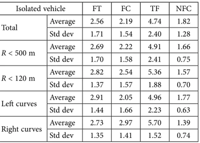
Table 1. Values of the FT, FC, TF and NFC indicators in an ‘isolated vehicle’ condition

Isolated vehicle FT FC TF NFC Total Average 2.56 2.19 4.74 1.82 Std dev 1.71 1.54 2.40 1.28 R < 500 m Average 2.69 2.22 4.91 1.66 Std dev 1.70 1.58 2.41 0.75 R < 120 m Average 2.82 2.54 5.36 1.57 Std dev 1.37 1.57 1.88 0.70

Left curves Average 2.91 2.05 4.96 1.77

Std dev 1.44 1.66 2.23 0.63

Right curves Average 2.73 2.97 5.70 1.39

Std dev 1.35 1.41 1.52 0.74

Table 2. Values of the FT, FC, TF and NFC indicators in a ‘disturbed vehicle’ condition

Disturbed vehicle FT FC TF NFC Total Average 2.88 3.81 6.69 1.75 Std dev 1.69 4.57 4.38 2.42 R < 500 m Average 2.82 4.14 6.96 1.49 Std dev 1.71 4.46 4.34 2.19 R < 120 m Average 3.07 3.91 6.98 1.75 Std dev 1.72 2.96 3.57 0.78

Left curves Average 2.61 4.42 7.03 1.86

Std dev 0.57 3.22 3.32 0.86

Right curves Average 4.29 2.54 6.83 1.48

Std dev 1.90 5.01 0.55 0.00

These results, even if already significant, have been further improved and refined, according to the charac-teristics of the objects seen while driving. Consequently, these entities have been firstly classified into static, dy-namic, and signage ones. Inside these categories, the static objects have been differentiated into parked cars and rubbish bins. Instead, the dynamic objects include the various vehicle types (cars, motorcycles, bicycles), categorized for the different directions. In the signage analysis, the authors evaluated both the vertical and the horizontal road signs, separating the danger warning, regulatory, guide, and work zone ones.

The results provided in Tables 3–5 report the fol-lowing data:

– ‘stimulus’: total duration in seconds of the stimu-lus potentially visible by the driver;

Figure 1. Relationship between geometric curve and duration of the glance on the internal edge of the curve

Tangent Tangent

TF

FT NFC

FC

Start observation End observation Curve

(5)

– ‘observation [s]’: total duration in seconds of the actual fixation of the stimulus;

– ‘observation [%]’: total duration of the actual fixa-tion divided by the total durafixa-tion of the stimulus; – ‘average [s]’: mean value of all the fixations

re-lated to the selected object for the whole road. The unseen objects have a duration equal to zero sec-onds and produce a decrease of the sample average value. In the bottom of Tables 3–5, the authors present the glob-al duration of the actuglob-al fixation for the various objects, compared to the total theoretical duration of the stimu-lus, in percentage. This information is further differenti-ated. The authors provide the total value, the actual fixa-tion along tangents, and the actual fixafixa-tion along curves. The wide differences in the results provided in Tab-les 3–5 confirm how it is worthwhile to separate the data, since a global analysis would hide precious information. For this reason, it is important to provide a small clari-fication. The researchers needed to identify not only the type of the dynamic object, but also the total time in

which it was effectively in the driver’s visual framework. Obviously, as a way of example, a bicycle in the same direction of a monitored driver is felt as a danger not only because it reduces the net transversal section, but also because of the longer time during which it is inside the visual framework. The visual behaviour evaluation becomes clearer by seeing some particular example im-ages, presented in the following (Figures 2–6).

3. Discussion

The results listed in Tables 1–5 are very significant and provide detailed indications about the actual driver’s visual behaviour. The aim of this research was to evalu-ate the influence on the driver’s behaviour of the distur-bances caused by various elements in the road context. It is important to underline that if the results can assess that this influence is relevant, it could be reasonable and appropriate to consider reformulations and modifica-tions in the design philosophy adopted by the major part of the countries, based on the ‘isolated vehicle’.

Table 3. Characteristics of the driver’s glance about the static objects during the travel Static objects

Stimulus [s] Observation [s] Observation [%] Average [s]

Total duration 7316.37 36.57 0.50 0.57

Stationary vehicle 3675.43 24.27 0.66 0.62

Rubbish bins 3640.93 12.30 0.34 0.49

Observed stimulus [%] 20.2

Observed stimulus in tangent [%] 17.1

Observed stimulus in curve [%] 38.0

Table 4. Characteristics of the driver’s glance about the dynamic objects during the travel Dynamic objects

Total duration 199.60 57.97 29.0 1.09

Car in the opposite way 95.30 28.53 29.9 1.19

Motorcycle in the opposite way 5.83 1.40 24.0 0.47

Bicycle in the same way 41.03 18.57 45.2 3.09

Car from entering 9.00 4.17 46.3 2.08

Pedestrian 3.50 1.37 39.0 1.37

Observed stimulus in curve [%] 42.0

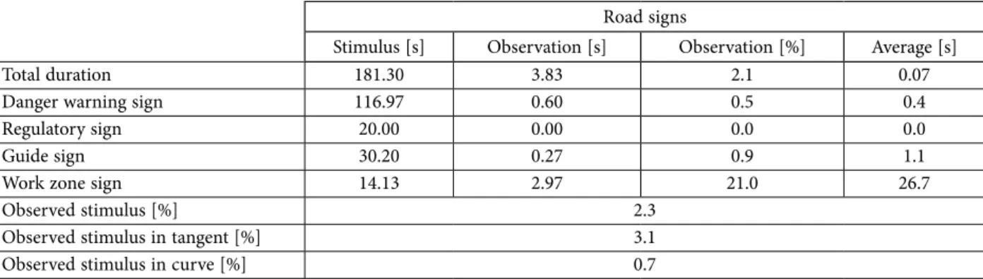
Table 5. Characteristics of the driver’s glance about the vertical signs during the travel Road signs

Total duration 181.30 3.83 2.1 0.07

Danger warning sign 116.97 0.60 0.5 0.4

Regulatory sign 20.00 0.00 0.0 0.0

Guide sign 30.20 0.27 0.9 1.1

Work zone sign 14.13 2.97 21.0 26.7

(6)

Tables 1 and 2 show the driver’s visual strategy through the quantification of FT, FC, TF, and NFC in-dices in both the scenarios of ‘isolated vehicle’ and ‘dis-turbed vehicle’. Some interesting aspects can be deducted from Table 1:

– the standard deviation of all the indices in the several configurations (as a function of the curve radius or direction) is very small; this confirms a good statistical consistency of the data;

– in the case of ‘isolated vehicle’, the FT average (it indicates the early fixation of the curve inner edge from the tangent) ranges between 2.56 and 2.91 seconds. In general, the authors may con-sider that this parameter is constant regardless the specific scenario. In the present experimen-tation, it seems that the driver starts to acquire information about the curve at least 2.5 seconds before its beginning. This time is very different from the value of 1 second proposed by other au-thors (Land 2006, 2010). Probably, since in this study the tests were performed in a real environ-ment rather than in a simulator, the authors can estimate the effect of numerous elements that, perhaps unawares, increase the complexity of the scenario to be interpreted (Figures 2–3), deter-mining this difference in the observation time; – the duration of the inner edge observation,

meas-ured by TF, presents some consistency with the boundary conditions changing. There is only a small increase while driving along tight curves (R < 120 m) and right curves. Both the condi-tions, intuitively, extend the fixation duration: in the first case, this is due to the greater difficulty to understand the curve; in the right curves, the horizontal signage is less deteriorated and thus it is a sure and reliable reference point for the user (Figure 3).

Table 2 is related to a vehicle disturbed by a series of static and dynamic entities. First of all, these elements have overall been evaluated in Table 2, while their sin-gle influence has been proposed in the following tables. Table 2 permits to examine the road scenario role rather than the external factor contribution. In addition, in this case, for more clarity, the considerations are provided using a bulleted list:

– the standard deviations are quite low;

– the FT index (curve Fixation along Tangent), in comparison to the ‘isolated vehicle’ case, is in-creased by a negligible amount. Only the right curves show a substantial increase (from 2.73 to 4.29 seconds), confirming that if the visual framework complexity grows, the driver looks for a reference point (the inner edge) as reliable as possible;

– on the contrary, the TF index is really higher than the ‘isolated vehicle’ value (about 2 seconds). This denotes that, due to the interpretation difficulties caused by the traffic, the driver needs a greater time to acquire the information from the inner edge. This increment in duration does not seem to be related to the curve radius or direction. Figure 6. The work zone signage is properly gazed,

even if its position close to the inner edge of the curve has facilitated this task

Figure 2. The fixations converged into the inner edge of the left curve

Figure 3. The fixation converged into the edge of the right curve (the vertical signs are ignored)

Figure 4. The vehicle coming in the opposite direction, without other stimuli, is seen by the driver

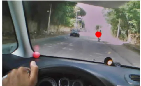
Figure 5. The driver’s eyes are on the bicycle in his same lane rather than on the car coming in the opposite direction,

(7)

The qualitative conclusions concerning the inves-tigated phenomenon are certainly intuitive and share-able. However, the experimentation allowed the authors to quantify the various user’s behaviours. In this way, it was possible to separate situations that did not induce relevant consequences with traffic variations (as the in-ner edge fixation in advance) from those much more influent on the driving performance (the increase on the total duration of the inner fixation).

Tables 3–5 contain further remarkable hints for the analysis. In detail, Table 3 focuses on static objects. These are only represented by parked vehicles and rub-bish bins at the roadside and, sometimes, slightly within the lane. Their fixation is justified since the driver feels them as a potential danger or, at least, as a bond point to carefully look at. The numerical examination leads to some conclusions that could be easily summarised as follows:

– although these elements are clearly visible for a long time (column ‘Stimulus’), the related driv-er’s fixation is very short (between 0.49 and 0.62 seconds – column ‘Average [s]’). Then, it could be stated that this task does not aggravate the cognitive process against other more complex elements;

– the parked vehicles are gazed for a time almost twice than the bins (0.66 against 0.34%). The au-thors believe this may be due to their different nature: the bin certainly represents something static, while the vehicle could hypothetically overrun the lane. For this reason, the drivers feel the stationary cars much more as a danger for their safety;

– their position along the road is very signifi-cant. The objects placed along the tangents are quickly identified, while the user spent more time for those positioned along curves (38.0 ver-sus 17.1%). This is a symptom confirming that the curve is always the geometric element more complex to interpret.

Table 4 provides outcomes for dynamic objects. The main considerations are listed in the following:

– it is easy to note a great fixation time not only in terms of absolute value, but in particular as a per-centage of the available stimulus. Obviously, this value is relatively short (especially for vehicles moving in the opposite direction), but percent-age fixations between 29.0 and 46.3% have been reached. In the previous table about static objects (Table 3), these data are limited to 1% and, thus, this is a clear indication that something dynamic into the road section is considered more danger-ous than a static element at the roadside; – the values listed in the third column

(‘Observa-tions [s]’) can be consequently seen as a classifi-cation of the dynamic object influence, unknow-ingly performed by the driver depending on the potential and dangerous interaction between the observed element and his car. This result is very

valuable, as it represents the ratio of the fixation duration by the total appearance of the object into the visual framework. In short, if this value is low, the driver retains the stimulus unimpor-tant for his transit and he neglects it, even if it is fully available into the visual framework. In the experimentation, the authors measured a value equal to 24.0 and 29.9% respectively for motor-cycles and cars coming in the opposite direction, 45.2% for bicycles moving in the same lane, and 46.3% for vehicles from entries. The monitored driver thinks, rightly, that the bicycle may reduce the net transversal section available for his mo-tion, because of its twisting trajectory. Moreover, the vehicle coming from another road could get a trajectory causing a critical collision;

– according to previous data, the authors have measured low relevance for motorcycles (0.47 seconds) and slightly higher (1.19 seconds) for car moving in the opposite direction (Figure 4). This time substantially increases for bicycles (Figu re 5) in the same lane (3.09 seconds) and for cars trying to take the same lane (2.08 seconds); – in this case also, the element fixation along the

curve is higher than along tangents (42.0 versus 29.1%).

The signage needs a specific interpretation and analysis. The authors know it is generally disregarded and ignored, but they would expect better results than those obtained. It is possible to evidence that:

– the percentages about the vertical sign fixations are derisory and do not reach the threshold of 1.0%. The kind of sign does not matter, because danger warning, regulatory, and guide signs show similar values;

– the only exception is due to the work zone sig-nage. In this case, the fixation time is remarkable (2.97 seconds), with a percentage of 21.0% com-pared to the stimulus duration.

Regarding the geometric element where the sig-nage is placed, the user favours the road signs in the tangents (3.1%), ignoring almost all those positioned in curves (0.7%). It means that in very complex scenarios such those characterizing curves, the driver discards the information that he considers not very significant. The road administrators could take care also to the fixa-tion times of these objects. Using these data with the users’ operative speeds, the designers could mitigate or improve the building elements of the infrastructure, in order to make them easier to understand.

However, the short time measured for the signage may also be related to the quick human cognitive pro-cesses, since the road signs are automatically recognized by users. This recognition is so fast, because these images are already seen and known by the driver and, thus, the information is sudden available for the brain. This evi-dence confirms the role of objects already tested against those needing a more laboured cognitive process.

(8)

Conclusions

The aim of this research was to evaluate quantitatively the various visual strategies of a driver moving on a ru-ral two-lane road. The remarkable variables investigated were various disturbing elements present in the visual framework, classified in this context into static (such as parked cars, rubbish bins, and signage) and dynamic ob-jects (all the vehicles, categorized by type and direction). The final outcomes seem to be very precious. Clearly, the sample size adopted for the test could be increased, but the available data allowed the authors to assess the visual behaviour in some specific scenarios, selected as a function of curve radius and direction (right or left) or element type.

The descriptive conclusions may appear obvious (for instance, the authors measured a greater fixation time of the curve inner edge with bicycles in the same lane), but since these are supported by numerical data (in terms of time, length, and fixation percentage), the results could be applied in many practical and theoreti-cal applications.

The applications may be numerous: first of all, in the traditional road management, the proposed proce-dure permits to evidence the sections hardly compre-hended by the users (high acquisition times), and to mitigate the related danger through proper operations, such the renovation of the margin lines, the increase of the sight distance by removing some obstacles, the driv-ing bans for some vehicles, or the definition of lower legal speed limits. Moreover, a deeper analysis of the signage fixations, could favour the definition of appro-priate methods for optimizing the road signal position. The collected data, properly examined together, may be used for driving forecasting models useful to evaluate the visual strategies of drivers in rural roads. In particu-lar, by varying the curve radius or deleting a specific disturbing element, it could be possible to presume the driver’s reactions, without exposing users to actual driv-ing in dangerous conditions.

In conclusion, these models, improved using specif-ic artifspecif-icial intelligence techniques, could also represent the starting point for building new systems and devices for intelligent transportation systems.

References

Bongiorno, N.; Bosurgi, G.; Pellegrino, O. 2016. A procedure for evaluating the influence of road context on drivers’ visual behaviour, Transport 31(2): 233–241.

https://doi.org/10.3846/16484142.2016.1188852

Bosurgi, G.; D’Andrea, A.; Pellegrino, O. 2015. Prediction of drivers’ visual strategy using an analytical model, Journal of

Transportation Safety & Security 7(2): 153–173. https://doi.org/10.1080/19439962.2014.943866

Bosurgi, G.; D’Andrea, A.; Pellegrino, O. 2010. Could drivers’ visual behaviour influence road design?, Advances in

Trans-portation Studies: an International Journal 22: 17–30.

Bosurgi, G.; D’Andrea, A.; Pellegrino, O. 2013. What variables affect to a greater extent the driver‘s vision while driving?,

Transport 28(4): 331–340.

https://doi.org/10.3846/16484142.2013.864329

Dijksterhuis, C.; Brookhuis, K.A.; De Waard, D. 2011. Effects of steering demand on lane keeping behaviour, self-reports, and physiology. A simulator study, Accident Analysis &

Pre-vention 43(3): 1074–1081.

https://doi.org/10.1016/j.aap.2010.12.014

Donges, E. 1978. A Two-level model of driver steering behav-ior, Human Factors: the Journal of the Human Factors and

Ergonomics Society 20(6): 691–707.

Habibovic, A.; Tivesten, E.; Uchida, N.; Bärgman, J.; Aust, M. L. 2013. Driver behavior in car-to-pedestrian incidents: an application of the driving reliability and error analysis method (DREAM), Accident Analysis & Prevention 50: 554–565. https://doi.org/10.1016/j.aap.2012.05.034 Jamson, A. H.; Merat, N.; Carsten, O. M. J.; Lai, F. C. H.

2013. Behavioural changes in drivers experiencing highly-automated vehicle control in varying traffic conditions,

Transportation Research Part C: Emerging Technologies 30:

116–125. https://doi.org/10.1016/j.trc.2013.02.008 Land, M. F 2010. The visual control of steering, in L. R. Harris,

M. Jenkin (Eds.). Vision and Action, 163–180.

Land, M. F. 2006. Eye movements and the control of actions in everyday life, Progress in Retinal and Eye Research 25(3): 296–324. https://doi.org/10.1016/j.preteyeres.2006.01.002 Lehtonen, E.; Lappi, O.; Kotkanen, H.; Summala, H. 2013.

Look-ahead fixations in curve driving, Ergonomics 56(1): 34–44. https://doi.org/10.1080/00140139.2012.739205 Martens, M. H. 2011. Change detection in traffic: Where do

we look and what do we perceive?, Transportation Research

Part F: Traffic Psychology and Behaviour 14(3): 240–250. https://doi.org/10.1016/j.trf.2011.01.004

Minin, L.; Benedetto, S.; Pedrotti, M.; Re, A.; Tesauri, F. 2012. Measuring the effects of visual demand on lateral deviation: A comparison among driver’s performance indicators,

Ap-plied Ergonomics 43(3): 486–492.

https://doi.org/10.1016/j.apergo.2011.08.001

Pellegrino, O. 2009. An analysis of the effect of roadway design on driver’s workload, The Baltic Journal of Road and Bridge

Engineering 4(2): 45–53.

https://doi.org/10.3846/1822-427X.2009.4.45-53

Pellegrino, O. 2012. Prediction of driver’s workload by means of fuzzy techniques, The Baltic Journal of Road and Bridge

Engineering 7(2): 120–128.

https://doi.org/10.3846/bjrbe.2012.17

Wege, C.; Will, S.; Victor, T. 2013. Eye movement and brake reactions to real world brake-capacity forward collision warnings: a naturalistic driving study, Accident Analysis &

Prevention 58: 259–270.