Giuseppe Castro
STUDY OF INNOVATIVE PLASMA HEATING METHODS AND APPLICATIONS TO HIGH CURRENT ION SOURCES
PhD Thesis
Tutors:
Prof. Francesca Rizzo Dott. Santo Gammino Dott. David Mascali PhD coordinator:
Prof. Francesco Riggi
Introduction vii
1 Fundamental of plasma physics 1
1.1 Plasma parameters . . . 1
1.2 Collision in plasmas . . . 2
1.2.1 Spitzer collisions . . . 2
1.2.2 Binary collisions . . . 4
1.2.3 Cold, warm and hot electrons in plasmas . . . 7
1.2.4 Recombination effects . . . 8
1.2.5 Remarks about collisions . . . 8
1.3 Theoretical approach to the plasma physics . . . 10
1.3.1 The single particle approach . . . 10
1.3.2 The kinetic approach . . . 11
1.3.3 The Magneto-Hydro-Dynamics (MHD) Approach . . . 12
1.3.4 Some applications of MHD equations . . . 15
1.4 Particle motion in a magnetized plasma . . . 16
1.4.1 Drift effects in plasmas . . . 18
1.5 Plasma diffusion . . . 21
1.5.1 Free diffusion . . . 21
1.5.2 Ambipolar diffusion in a magnetized plasma and short-circuit effects . . . 22
1.6 Plasma confinement . . . 25
1.6.1 The simple mirror configuration . . . 25
1.6.2 The B-minimum configuration . . . 29
2 Waves in plasmas 31 2.1 Propagation of E.M. waves in plasmas . . . 32
2.1.1 E.M. waves in a cold-unmagnetized plasma . . . 32
2.7 Absorption of E.S waves . . . 69
2.7.1 Landau Damping . . . 69
2.7.2 The Sagdeev and Shapiro damping . . . 71
2.8 Remarks about EBW heating . . . 72
2.9 Remarks about wave propagation in plasmas . . . 72
3 Introduction to the ion sources and beam characteristics 75 3.1 Ion sources requirements . . . 76
3.2 Principal ion sources . . . 77
3.3 ECR-based ion sources . . . 79
3.3.1 ECRIS . . . 80
3.3.2 MDIS . . . 83
3.4 Ion sources at INFN-LNS . . . 86
3.5 Beam parameters . . . 88
3.5.1 Emittance and Brightness . . . 88
3.5.2 Space charge effects . . . 90
4 Experimental equipment and diagnostics 93 4.1 The plasma reactor . . . 94
4.2 The Versatile Ion Source (VIS) . . . 96
4.3 Plasma diagnostics . . . 103
4.3.1 Langmuir probe diagnostics . . . 104
4.3.2 OML approach . . . 107
4.3.3 X-ray diagnostics . . . 112
5 Plasma heating in higher harmomics 121
5.1 Measurements set-ups . . . 122
5.1.1 Results obtained when using the magnetic beach con-figuration . . . 124
5.1.2 The flat-B field configuration . . . 134
5.2 Plasma heating at 2.45 GHz in plasma reactor . . . 140
5.2.1 Ray Tracing modelling . . . 144
5.3 Spectral emission analysis . . . 154
5.4 X ray spectroscopy . . . 157
5.5 Plasma imaging in optical and X rays domain . . . 162
5.6 Influence of the magnetic field configuration on hot electrons population . . . 164
5.7 Influence of under-resonance plasma heating on the electron energy content . . . 168
The use of plasmas in various areas of scientific research has been growing in recent years. Since 1970, moreover, their contribution has been crucial in the field of accelerator physics, and consequently contributed to the impulse that this gave to nuclear and Particle Physics in the last thirty years. The Electron Cyclotron Resonance Ion Sources and the Microwave Discharge Ion Sources are currently the best devices worldwide able to feed effectively high energy accelerators such as Linacs, Cyclotrons, Synchrotrons or Colliders. The plasma is excited by microwaves typically in the range 2.45-28 GHz; microwaves are coupled to a cylindrical chamber working as resonant cav-ity, where the plasma is produced, by a suitable system of waveguides, and are absorbed therein during the interaction with gases or vapors fluxedd at low pressure (10−6 - 10−3 mbar). In presence of the magnetostatic field, the electromagnetic wave absorption is particularly efficient at the so-called ”Electron Cyclotron Resonance”. From the high density and high temper-ature plasma (ne ∼ 1010− 1012cm−3, Te ∼ 0.1 − 100keV ) part of the ion
content is extracted, which finally constitutes the ion beam to be sent to the accelerators. Most of the parameters of the extracted beam, such as the intensity, the emittance and the shape in the real space depend in a deci-sive way on the characteristics of the plasma which from which the beam is extracted. The further development of ECR-type ion sources is however intrinsically limited by physical properties of the plasmas. The electromag-netic energy can not be transferred to the plasma electrons over a certain density threshold, named cutoff density, (in other words, the layer in which the ECR resonance occurs becomes inaccessible). Normally, in plasmas sus-tained by microwaves, the density increases with RF power but it stabilizes below a limit value situated just slightly below the critical density. In the field of controlled nuclear fusion and magnetic confinement, this topic has a crucial importance since it limits the satisfaction of the Lawson criterion. But also in the ion sources field this topic is of fundamental importance,
static oscillations (conversion mechanisms are typically called XB or OXB mechanisms). We operated in different experimental conditions: by varying the operating frequency (by means of a TWT), it is possible to operate ex-clusively in EBW heating mode, to have the simultaneous presence of ECR heating and EBW heating or, opportunely moving the permanent magnets, totally inhibited the generation of electrostatic waves. EBW generation and absorption in a plasma is highlighted by the three experimental evi-dences: 1) exceeding of the electromagnetic density cutoff 2) generation of high-energy electrons, 3) detection of non-linear decay of the spectrum of the incident electromagnetic radiation in a plurality of ancillary frequencies (the ”broadening” of the incident electromagnetic radiation is often referred as ”parametric decay”). All these three signatures have been measured above a critical threshold of the RF power (further sign of non-linear interaction). The study of the high energy electrons population has been carried out by means of the bremsstrahlung radiation emitted by the electrons when col-liding with the plasma ions or with the chamber walls. The detection of X radiation at energies domains of tens of keV is absolutely relevant by a sci-entific point of view, and it represents one of the clue of this thesis work. In facts, generally MDIS plasmas are not capable to emit in the X-ray domain (the maximum energy of the electrons is typically 100-200 eV in ECR heat-ing regime). When satisfyheat-ing conditions for modal conversion, the formation of a plasma ”vortex” was moreover observed. Drifting electrons are char-acterized by an electron speed of the order of 1 · 106m/s due to absorption of electrostatic waves at cyclotron harmonics (measurements say). At the moment we are able to demonstrate only that an electronic azimuthal flow exists, but some experimental data and the ongoing studies would suggest that an ion motion is excited too.
The arguments up to now introduced were organized in five different chap-ters: In the first chapter we introduce the general features of plasmas, as the collisional effects, the diffusion and the different theoretical approaches to model magnetized plasmas in linear machines. The second chapter is de-voted to problems related to wave propagation in magnetized plasmas. To a first part dedicated essentially to the propagation of electromagnetic waves, the study of the generation and absorption of the Bernstein waves in plasmas will follow. In the third chapter an overview of the different ion sources is given, together with the main peculiarities of the microwave discharge and ECR ion sources. Furthermore the basic parameters that characterize the particle beams are defined. The fourth chapter introduces the experimental apparatus used for measurements and provides an overview of the analysis methods used to derive the plasma parameters. Chapter 5 shows the anal-ysis of the experimental data in terms of profiles density, X spectroscopy and spectral analysis of electromagnetic radiation interacting with plasmas. The space resolved analysis of the plasma resistivity curves provided in-formation on the density profiles and electron temperature, highlighting a substantial increase in the regions of magnetic field favorable to the occur-rence of the modal conversion. Thanks to the systematic study of the X-ray spectra it was moreover possible to identify the threshold of the conversion process (∼ 80 W for the specific set-up), characteristic of all the non-linear processes that occur beyond certain values of RF power. Finally, the con-clusion chapter of the thesis is aimed to identify the possible applications of the how developed in this thesis; in particular the gained know-how has potential applications in the design and construction of the injector of the European Spallation Source facility and for the project DAEδALUS (Decay At rest Experiment for δ CP studies At the Laboratory for Under-ground Science). The obtained results are of particular importance also in a far future perspective, since conceptually new ion sources could be realized starting from the new mechanism of plasma heating hereby investigated.
Fundamental of plasma
physics
The plasma physics is one of the fundamental branch of modern science. It finds a great number of applications in several fields of nature, from astrophysics to nuclear physics, to the applications to the nuclear fusion and to the industrial applications. Plasma constitutes over the 98% of the matter of the universe. Thus, the study of plasma physics can provide a fundamental step forward in the comprehension of the nature. In the next pages only the aspects directly linked to the activities carried out during the PhD course will be treated with some details. A more detailed and generalized treatment can be found in the references [1] and [2].
1.1
Plasma parameters
The fundamental parameters characterizing the plasmas generated in an Electron Cyclotron Resonance Ion Source are the electron density ne
(mea-sured in cm−3or m−3), the temperature T of each species (usually measured in eV or keV ), the ion confinement time tc and the external magnetic field
B.
All the main characteristics of the plasma and of the extracted beam de-pend on these four parameters. Several ancillary parameters can be derived from these and they will be introduced little by little in the following. The Debye length represents the scalelength over which mobile charge carriers (e.g. electrons) screen out electric fields in ionized gas:
Plasma collisionality plays a crucial role in several processes. It regulates the confinement times in magnetically confined plasmas, it thermalizes the electrons in low temperature discharges and it determines the ionization rates in a plasma used as source of ions. In order to discuss about the main collision phenomena occurring in ECR plasmas, it is convenient to introduce two physical quantities: the mean free path λmf pand the collision frequency
ν. These parameters depends on the cross section of the process σ [2]: λmf p=
1
nσ (1.2.1)
ν = nσv (1.2.2)
where σv is the product between the cross section and the particle veloc-ity averaged over the velocveloc-ity distribution function (generally a Maxwellian one). The collision time τ is the reciprocal of the collision frequency τ = 1/ν. The collisions occurring in plasma can be divided in two groups according to the number of colliding particles: multiple collisions are characteristics of plasmas, because they occur thanks to the long range Coulomb interac-tion. The binary collisions are similar to the collisions in gaseous systems; however, in this case, non-elastic and ionizing collisions occur because of the high energy content of the plasma particles, especially of electrons.
1.2.1 Spitzer collisions
The Spitzer collisions represent the multiple interactions of a single parti-cle with many other partiparti-cles, and the net effect is to give a large-angle scattering. These cumulative small-angle scatterings, finally resulting in a 90◦ deflection, play a role only in highly ionized and low pressure plasmas,
where internal electromagnetic interactions are predominant. These colli-sions must be extended over the whole distance where the Coulomb forces are effective, i.e. the Debye shielding length. It can be demonstrated that the effective cross-section for 90◦ deflection by means of multiple collisions is [2]: σ = z1z2e 2 ϵ0mv2 2 ln λd bmin (1.2.3) where z1 and z2 are the charges of the two particles, e is the electron
charge, m is the mass of the colliding particle and the term ln λd bmin
= ln Λ is the so called Coulomb logarithm. This equation is similar to the cross-section for single Coulomb scattering (Rutherford formula), but the multiple scattering probability exceeds single scattering by the factor 8 ln Λ, so the 90◦ scattering due to a single collision is much less probable than multiple deflections. Starting from equation (1.2.3) it is possible to calculate the collision frequencies for the different particle constituting the plasma:
ν90ee◦ = 5 · 10−6ne ln Λ T 3 2 e (1.2.4) ν90ei◦ ∼= 5 · 10−6zne ln Λ T 3 2 e (1.2.5) ν90ii◦∼= z4 me mi te ti 3 ν90ee◦ (1.2.6)
where ne is in cm−3 and Te in eV . Each frequency is usually called
charac-teristic Spitzer collision frequency1.
The first consequence of the previous equations is that ν90ii◦ ≫ ν90ee◦ ∼ ν90ei◦,
i.e. the ions are much more collisional than electrons. In a MDIS plasma characterized by a density of 1 · 1011cm−3 and Te= 10 eV, νee lies between
105 and 106Hz. Because the cyclotron frequency usually ranges between
2.5 and 20 GHz, Spitzer collisions does not prevent the electron gyromotion around the force lines of the magnetic field. For this reason, ECR plasmas can be considered collisionless or quasi-collisionless, and this remains true in most cases even when inelastic and elastic collisions are added to the Spitzer collisions. To investigate the plasma thermalization via collisions
1The correct term should be 90◦
scattering. We talk about the collision frequency for sake of simplicity.
nal electromagnetic field. This result is of primary importance for ECRIS, as one of the most important quality parameters, the emittance, increases with the ion temperature. Thermalization of electrons can be explained by means of the collisions only for low electron energy (few eV ). For larger energies τmeebecomes larger than the plasma lifetime and the thermalization can be explained only taking into account stochastic processes due to the interaction of the electrons with the electromagnetic wave.(see section 2.2).
1.2.2 Binary collisions
The binary collisions in plasmas can be divided into two groups: the electron-neutral collisions (elastic and inelastic), and the ionizing collisions. The for-mer plays an important role especially in case of high pressure plasmas with a low degree of ionization and a low electron temperature2 [2]. As featured in figure , these collisions provide the thermalization playing the same role of the Spitzer collisions in case of highly ionized and low pressure plasmas. At electron temperatures comparable or higher than the neutral ionizing po-tential, the ionizing collisions becomes the most important collision. Even if multi-ionizing collisions might occur, the process having the larger cross section is the single ionization3, also called step-by-step ionization. The time needed for the transition from charge state z1 to charge state z2 by
means of single ionization takes a time, on average, is [2]: τz1z2 = 1 neσz1z2v (1.2.7) 2 P ∼ 10−3− 10−4 mbar, Te≤ 15eV.
3The cross section to expel two electrons is one order of magnitude lower than single
Averaging over a Maxwellian distribution, we find: τz1z2 =
1 neS(Te)
(1.2.8) where S(Te) is the reaction rate coefficient which depends only on the
temperature of the electron distribution function. Only if the ion confine-ment time tcis longer than the time required for the given ionization,
tran-sition z1 → z1 takes place. From the condition tc> τz1z2 we obtain:
neτc≥
1 S(Te)
(1.2.9) Equation (1.2.9) can be rewritten by substituting the S(Te) parameter,
ob-taining: ζneτc≥ 5 · 105Teopt 32 (1.2.10) where ζ = j
qj is the number of subshells in the atom outer shells and
Teopt∼ 5Wthr is the optimal temperature to have ionization, about equal to
five time the ionization threshold energy Wthr. The product neτc is called
quality factor for ion sources and, together with the electron temperature, it determines the performances of the ion source. This means that it is possible to improve the performances of an existing source by opportunely increasing these three fundamental parameters. In figure 1.2.1 the function neτc = f (topte ) together with the main ions obtainable in such conditions.
The increase of the quality factor and of electron temperature through the development of new plasma heating methodic represents the main frontier of the research and one of the main goals of the PhD activity.
Figure 1.2.1: Golovanivsky’s diagram shows the criteria for the production of highly charged ions. The ions enclosed by circles are completely stripped; some combinations of electron temperature, electron density and ion confinement time allow to produce completely stripped ions; inside brackets uncompletely stripped ions are shown: they can be produced with the corresponding plasma parameter of ions enclosed in circles [2]
1.2.3 Cold, warm and hot electrons in plasmas
Equations (1.2.4-1.2.6) show the strong dependance of the collision frequency on the electron temperature. As the electron temperature increases, the Spitzer collision probability decreases significantly. A complete thermal-ization of the electrons is therefore impossible, and three different electron populations, usually named cold, warm and hot electrons, are present at any time within the plasma. The characteristics range of energy of each popu-lation depends on the type of ion source used. For example in ECRIS the cold population is characterized by temperatures in the range of 1-100 eV, the warm in the range of 100 eV-100 keV, and the hot above 100 keV [2]. On the contrary, in a MDIS the characteristic energy of each population is much lower. As it will be shown in chapter 5, we reveal a cold elec-trons population having energy of 1-10 eV, warm elecelec-trons of several tens or hundreds of eV and a hot population with energies larger than 1 keV. In general the most important population is the warm component. In facts it has an energy large enough to ionize the atoms up to high charge states and, at the same time, a sufficient collision frequency. Only a small part of the cold electrons induce ionization in MDIS, and in ECRIS their energy is too low to ionize inner shells of atoms, even if their collision frequency is the highest. Finally, the hot electrons have a too low cross section for the ionization process, although they have high energies. Further they are detrimental for ECRIS, because they increase the aging of insulators and, in the case of third generation ECRIS, they can heat the helium cryostat, making the operations of the source difficult. The ideal working configura-tion for obtaining the best performances from an ECRIS is that one which maximizes the warm component while minimizing the hot component. On the contrary, in MDIS sources, the possibility to produce a large amount of hot electrons might be very interesting for different applications and it need to be further investigated. MDIS sources, in facts, are usually able to produce only monocharged ions4, and the generation of hotter electrons could enable the production of multiply charged ions. In the experimental and conclusions chapters these arguments and the related consequences for ECRIS and MDIS will be further explored.
4Their characteristic electron temperature and ion lifetime, is too low to allow the
the higher is the probability of charge exchange collisions increase with the number of particle of plasma. For high performance ion sources the charge exchange collision time must be longer than the ionization time for a given charge state, i.e. τexch> τz1z2. This implies that:
n0 ne ≤ 7 · 103ζA z T opt e 32 (1.2.11) where n0 is the density of neutrals, and A is the atomic mass number.
1.2.5 Remarks about collisions
The relative ratios of various neutral and ion species in ECR ion sources are determined by the dynamic balance between their generation and loss rates. According to the previous sections, the main processes which take to generation of an ion of charge state i and particle density ni are the step by
step ionization by electron collisions and the C.E recombination with higher ionized ions. The main processes which take to the losses of ni are the C.E
recombination with lower ionized ions or neutrals, the further ionization of the ion by means of electron impact and finally the losses due to diffusion and recombination on the plasma chamber walls5. The number of particles per unit volume created or destroyed by means of the different processes can be evaluated by means of the reaction rate coefficient Q, defined as:
Q) ∞
0
σf (v)vdv (1.2.12)
Where σ is the cross section of the process, and f (v) is the electron dis-tribution function. Q represents the number of reaction occurring per unit
5Ion extraction is implicitly included in the losses due to diffusion; in facts ions are
of interacting particles density per second. For practical uses, assuming a Maxwellian distribution, Q can be written as [84]:
Q = 6.7 · 107T− 3 2 e ∞ 0 EσeTeEdE (1.2.13)
Here Te and E are expressed in eV and σ in cm2. By definition of Q, it
follows that the number of reactions occurring in a cm3 per second is given by P = N neQ, where N and ne are the reaction particles densities. If the
cross sections of the different processes are known, it is hence possible to write a set of N balance equations depending on some free parameters: the electron density ne, the confinement time τi, the electron temperature Te:
∂ni ∂t = i−1 j=0 nenjQEIj→i+ i−1 j=0 zmax ν=i+1 njnνQCEj,ν→i− i−1 j=0 i−1 ν=1 njniQCEi→i−ν− zmax j=i+1 nenjQEIi→j − ni τi = 0 i = 1, 2, ..., zmax (1.2.14) where zmax is the highest charge number limited by the electron energy. To
close the equation system, it is then necessary to add the quasi-neutrality condition: ne= zmax i=1 qini (1.2.15)
where qi represents the charge state of the ion having particle density ni.
The number of neutral particles per unit volume n0 can be related to the
background pressure as:
P = n0Ti (1.2.16)
Ti being the ion temperature expressed in eV .
This model can be applied either to calculate the charge state distributions in an ECRIS [6] or the mass spectrum and the ionization degree in a MDIS [7]. In figure 1.2.2 the relative abundance of the Argon charge states as a function of jeτi. The main charge state increases for larger ion lifetime.
Figure 1.2.2: Relative abundance of the Argon charge states as a function of the confinement time (multiplied for the current density je), for an electron temperature
Te= 10 keV.
1.3
Theoretical approach to the plasma physics
The plasma is constituted by an enormous number of charged particle. A proton source operating at pressure of about 1 · 10−5mbar and one liter volume, for example, contains about 1015ions and electrons. It is practically impossible to solve the motion equation of all the particles or to take into account all the possible collisions between a so large number of particles. In a few words the theoretical approach to the plasma physics needs some approximations.
1.3.1 The single particle approach
The most simple approach to the study of the plasmas is based on the single particle dynamics. Many properties of plasmas, from the confinement to the energy absorption during the-wave particle interaction, and also many aspects of the electromagnetic field propagation can be described in terms of the single particle approach. This approach is based on the solution of the motion equation only for a small number of particles, called test particles (≈ 105), representative of all the particle constituting the plasma. The simplest equations describing the propagation of electrons and ions in a
plasma are respectively [3]: me d⃗v dt = e ⃗E + Fcoll+ e⃗v × ⃗B0 (1.3.1) mi d⃗v dt = Fcoll (1.3.2)
this equation takes into account the effects on the single particle motion, in a non relativistic approximation, of the wave electric field, of the magneto-static field and of the collisions. In the ion case, the interactions with the electric and magnetic field can be neglected because of their high collision-ality. The motion of ionized and neutral atoms is totally similar, in first approximation, to the Brownian motion. As in case of plasmas produced in ECR ion sources the electrons easily reach energies of the order of some hundreds of keV, or also MeV, the relativistic effects must be taken into account, and the complete single particle equation of motion becomes:
d⃗v dt = q m0γ ⃗ E + ⃗v × ⃗B.⃗v · ⃗E c2 ⃗v (1.3.3) where ⃗E is the electric field of the wave, and ⃗B is the sum of the wave magnetic field and of the magnetostatic field used for the plasma confine-ment.
1.3.2 The kinetic approach
The most detailed approach to the plasma dynamics is the kinetic the-ory, which is based on non-equilibrium thermodynamics. An exhaustive approach requires to know all the particle positions and velocities, the fields in which these particles are located and also the reciprocal interaction, or the correlations between pair or groups of particles. This treatment requires the introduction of the distribution function f (⃗r, ⃗v, t). The meaning of the distribution function is that the number of particles per m3 at position ⃗r and time t with velocity components between vx and vx+ dvx, vy and vy+ dvy,
vz and vz+ dvz is f (x, y, z, vx, vy, vz, t)dvxdvydvz.
As a consequence f (⃗r, ⃗v, t) is normalized so that: +∞
−∞
f (⃗r, ⃗v, t)d⃗v = N (1.3.4) where N is the total number of particle constituting the plasma.
sence of collision and by considering the acceleration as due exclusively to electromagnetic forces, the previous equation can be finally rewritten as:
∂f ∂t + ⃗v · ⃗∇rf + q m ⃗E + ⃗v × ⃗B · ⃗∇vf = 0 (1.3.6)
This equation is called Vlasov equation. When collisions can not be ne-glected, the total derivative of the distribution function is not zero, but equal to the time rate of change of f due to the collisions (∂f /∂t)c. The equation which takes into account the collisions is named Boltzmann equa-tion, and it is easily obtained from (1.3.6) by adding the collisional term:
∂f ∂t + ⃗v · ⃗∇rf + q m ⃗E + ⃗v × ⃗B · ⃗∇vf = ∂f ∂t c (1.3.7) Theoretically these equations should be solved for each plasma particle, subjected, point by point, to a well defined field depending on the position of the other particles. Fortunately the problem can be simplified by using the mean field approximation and by assuming the particle unrelated. In this approximation, the interaction between a particle and the other ones occurs only by means of the mean field created by all the particle of the plasma. The equation (1.3.6) describes the stationary plasma states, the plasma waves, the instabilities and other short time effects of plasma dynamics in terms of the distribution function f (⃗r, ⃗v, t).
1.3.3 The Magneto-Hydro-Dynamics (MHD) Approach
Although the plasma looks like a gas, it behaves more like a fluid, and the fluid mechanics is usually a powerful method to describe it. By means of the
MHD the plasma dynamics can be described without a precise knowledge of all the particle positions and velocities, but in terms of macroscopic parame-ters like temperature, density, pressure, etc. In this sense the fluid approach is simpler than the Vlasov one, and the collisions can be included by con-sidering the momentum exchange between electrons and ions. However all the microstructures due to particle effects cannot be taken into account by means of this approach. Collisionless absorption of electromagnetic waves, and other aspects concerning instabilities due to velocity-distribution inho-mogeneities, remain out from the fluidodynamics possibilities. MHD equa-tions can be obtained by making the momenta of equation (1.3.6)[1]. This approach produces a system of n equation in n + 1 unknowns, in facts each time a higher moment of the Vlasov or Boltzmann equation is calculated in an attempt to obtain a complete set of transport equations, a new macro-scopic variable appears. It is then necessary to introduce an acceptable simplifying assumption on the highest momentum closing the equations sys-tem.
In collisionless approximation, the first three moments are obtained by mul-tiplying the Vlasov equation by m, mv, and mv2/2, and integrating over all
the velocity space. The results are respectively:
1. the equation of conservations of mass (continuity equation); ∂n
∂t + ⃗∇ · (n⃗u) (1.3.8)
where ⃗u is the fluid velocity.
2. the equation of conservations of momentum (fluid equation of motion);
mn ∂u ∂t + (⃗u · ⃗∇)⃗u = qn ⃗E + ⃗u × ⃗B − ⃗∇ · ¯P¯ (1.3.9) ¯ ¯
P represents the stress tensor, whose components Pij = mnvivjspecify
both the direction of motion and the component of the momentum involved. When the distribution function is an isotropic Maxellian, ¯P¯ can be written as:
¯ ¯ P = p 0 0 0 p 0 0 0 p (1.3.10) In such a case ⃗∇ · ¯P = ⃗¯ ∇p.
there exist many conditions in which thermal velocity can be neglected. For this reason the cold plasma approximation will be used in chapter 2 to find the dispersion relation of electromagnetic waves propagating in the plasmas. The warm plasma approximation considers also the third momentum of Vlasov equation, i.e. the state equation, neglecting the heat flux tensor as in equation (1.3.11).
The complete set of MHD equations is obtained by adding the Maxwell equations to the (1.3.8), (1.3.9) and (1.3.11):
⃗ ∇ × ⃗E = −∂ ⃗∂tB ⃗ ∇ × ⃗B = µ0(niqi⃗vi+ neqe⃗ve) + µ0ϵ0∂ ⃗∂tE ∂nj ∂t + ⃗∇ · (nj⃗vj) j = i, e mjnj ∂⃗v j ∂t + (⃗vj · ⃗∇)⃗vj = qjnj ⃗E + ⃗vj× ⃗B − ⃗∇pj j = i, e pj = Cjnγjj j = i, e (1.3.12) The set of Equations (1.3.12) need to be solved either for the electron fluid and for the ion fluid. The divergence equations present in the set of Maxwell equations can be neglected because they can be recovered by making the divergence of curl equation.
The solution of the set of 16 scalar equation in the 16 unknowns ni, ne, pi,
fluid approximation.
If we take into account the plasma quasi-neutrality (i.e. ne ≃ ni), and we
neglect the ratio me/mi, we can consider only large scale and low-frequency
phenomena. We finally consider that the system remain isotropic at all times. These hypothesis enable us to add the set of equation for ions and electrons, obtaining the Single fluid MHD equations [1]:
⃗ ∇ × ⃗E = −∂ ⃗B ∂t (1.3.13) ⃗ ∇ × ⃗B = µ0⃗j (1.3.14) ∂ρ ∂t + ⃗∇ · (ρ⃗v) (1.3.15) ρ∂⃗v ∂t = ⃗j × ⃗B − ⃗∇p (1.3.16) ⃗ E + ⃗v × ⃗B = η⃗j (1.3.17)
where the (1.3.13) and (1.3.14) are the Maxwell equations, 1.3.15 is the mass continuity equation, the (1.3.16) is the momentum transport equation, the (1.3.17) is the Ohm’s law.
1.3.4 Some applications of MHD equations
Several physical concepts are easily gleaned from the MHD equations. For a steady state, from equations (1.3.16) and (1.3.14), it follows that:
⃗
∇p = µ−10 ⃗∇ × ⃗B
× ⃗B (1.3.18)
By simplifying the previous equation: ⃗ ∇ p + B 2 2µ0 = µ−10 ⃗B · ⃗∇ ⃗B (1.3.19) In many interesting cases, such as a straight cylinder with axial field, the right-hand side vanishes. In many other cases the right-hand side is small. Equation (1.3.19) then becomes:
p + B
2
2µ0
= constant (1.3.20)
Since B2/2µ0 is the magnetic field pressure, the sum of the particle pressure
2. β = 1: The diamagnetic effect generate an internal magnetic field exactly equal to the external one and two regions exist: one where only the magnetic field is present, the other where only the plasma, without magnetic field, exists;
3. β > 1: The plasma pressure is higher than that due to the magnetic field, then the plasma cannot be magnetically confined;
The magnitude of the diamagnetic current can be found by taking the cross product of equation (1.3.16) with ⃗B in the equilibrium case (∂/∂t = 0):
⃗j = B × ⃗⃗ ∇p
b2 = (KTi+ KTe)
⃗ B × ⃗∇n
b2 (1.3.22)
The ⃗j × ⃗B force generated by the diamagnetic current balances the pressure force in steady state and stop the motion, as shown in figure (1.3.1).
1.4
Particle motion in a magnetized plasma
In this section the motion of electrons and ions within a magnetized plasma will be analyzed by following the single particle approach discussed in sec-tion 1.3.1. In secsec-tion 1.2 it has been shown that collision frequencies have different importance for electrons and ions: electrons can be considered non-collisional while ions are strongly non-collisional.
The general motion equation for an electron moving in an external magnetic field in absence of collisions:
me
d⃗v
Figure 1.3.1: Diamagnetic current and magnetic field direction in cylindrically shaped plasma
The reference system can be defined in order to have the magnetic field oriented along the z axis, so that ⃗B can be written as ⃗B = B ˆz. The solution of equation (1.4.1) is then:
vx = v0⊥cos(ωct + φ)
vy = −v0⊥sin(ωct + φ) (1.4.2)
vz = vz0
where v0⊥ is the component of the velocity orthogonal to the magnetic
field, φ = arctan(−v0y v0x
) is the phase, and ωc is the cyclotron frequency:
ωc=
|q|B me
(1.4.3) Equation (1.4.2) tell us that electrons move along the direction of the magnetic field with helicoidal trajectories. The electron gyration radius, usually called Larmor radius is equal to:
rL=
mev⊥
|q|B (1.4.4)
Therefore, for electrons the space is no more isotropic and the presence of the magnetic field introduces a preferential direction along ˆz.
1.4.1 Drift effects in plasmas
External or internal forces can affect the motion of particles in a magnetized plasma. Such forces can be superimposed from outside7 or self-generated from inside the plasma8. Their effect is to modify the original cyclotron motion of the particle, adding a drifting component to the velocity.
Only the component of the force perpendicular to the magnetic field F⊥ has
importance in the resolution of the problem. The Fz component, in facts,
generates simply an acceleration along the z axis and it does not interact with ⃗B ( ⃗Fz× ⃗B = 0) For sake of simplicity, thus, we may choose ⃗F to lie in
the x − y plane. In presence of such force, the equation motion becomes: md⃗v
dt = q⃗v × ⃗B + ⃗F (1.4.6) It can be shown [1] that the solution of equation (1.4.6) is given by the sum between the velocity component of equation (1.4.2) and a constant vector.
To find the module and the direction of the drift velocity ⃗vdis hence sufficient
to solve equation (1.4.6) for the constant vector ⃗v = ⃗vd:
⃗
F + q⃗vd× ⃗B = 0 (1.4.7)
taking the cross product with ⃗B, one finds: ⃗
F × ⃗B + q⃗v × ⃗B × ⃗B = qvB2− q ⃗B(⃗v · ⃗B) (1.4.8)
6In reality also if < v >= 0, < v2> is ever different from zero, allowing ion diffusion. 7
For example, in RF ion sources[4], plasma is generated by means of a variable electric field superimposed to electron motion.
8In many cases[86], as the one described in the experimental chapters of this work, the
looking at the transverse component of ⃗v with respect to ⃗B, we finally have: ⃗vd= ⃗ F × ⃗B qB2 (1.4.9)
Equation 1.4.9 shows that the direction of ⃗vd depends on the sign of charge,
so in general ion and electrons, under the effect of the same force, drift in oppositive directions. As it was explained previously, in ECRIS and MDIS ions are unmagnetized, so they can not be affected by drift motions, depend-ing on the interaction between ⃗F and the effective magnetic field. However, if ion lifetime is long enough to allow momentum transfer among ions and electrons, the drifting electrons can accelerate ions via e − i collisions. In many practical cases, the force generating the electron drift is due to the action of uniform or a non-uniform electric field on plasma electrons. These two case will be treated separately. For sake of generality also drift effect on ions will be taken into account.
• Drift generated by an uniform electric field;
In such case equation (1.4.9) becomes:
⃗ vd=
⃗ E × ⃗B
B2 (1.4.10)
The drift velocity ⃗vdis independent of q, m and ⃗v⊥. Both ions and electrons
are drifted in the same direction with the same drift velocity whose module is |vd| = E/B.
• Drift generated by a non-uniform electric field;
Self-generated electric fields have often a wave behaviour and they gen-erally vary both in space and time as ⃗E = ⃗E0ei(⃗k·⃗r−ωt). For an arbitrary
variation of ⃗E in space, and a sinusoidal variation in time, it can be shown [1] that equation (1.4.10) can be rewritten as:
⃗ vd= ⃗ E × ⃗B B2 + 1 4r 2 L∇2 ⃗E × ⃗B B2 ± 1 ωcB d ⃗E dt (1.4.11)
In last term the sign ± stands for the signs of the particle charge.
If one assumes ⃗E varying sinusoidally also in space, the previous equation can be written as:
Figure 1.4.1: Motion of a charged particle subjected to an external magnetic filed ⃗
B and to an electric field ⃗E.
⃗ vd= ⃗ E × ⃗B B2 − 1 4r 2 Lk2 ⃗E × ⃗B B2 ± 1 ωcB d ⃗E dt (1.4.12)
Equations (1.4.11) and (1.4.12) show that the motion of the guiding center has two components, one perpendicular to ⃗B and ⃗E, and one directed along the direction of ⃗E. The first term of equation (1.4.11) corresponds to the drift velocity in case of uniform electric field. The second term is called the finite-Larmor-radius effect. Since rL is much larger for ions than for
electrons ⃗vd is no longer independent of species. However the effects due
to this term are important only for relatively large k (small wavelength) or small scale length of inhomogeneity. The third term is called polarization drift and it also depends on the charge of the particle. It is directed along the direction of the Electric field and it tends to separate ions from electrons. When a field ⃗E is suddenly applied, for example, ions move in direction of
⃗
E, while electrons will move in the oppositive direction. The polarization effect in a plasma is similar to that in a solid dielectric, where ⃗D = ϵ0E + ⃗⃗ P .
The dipoles in a plasma are ions and electrons separated by a distance rL.
The polarization current generated by the oppositive motion of ions and electrons (for Z=1) is:
⃗jp= ne(vip− vep) = n B2(mi+ me) d ⃗E dt ∼ = mi B2 d ⃗E dt (1.4.13)
quasi-neutrality, the application of a steady ⃗E field does not result in a polar-ization field ⃗P . However, if ⃗E varies sinusoidally as ⃗E = ⃗E0eiωt, then an
oscillating current ⃗jp results from the lag due to the ion inertia. In such a
case the polarization current ⃗jp will be:
⃗jp=
minω
B2 E⃗0e
iωt (1.4.14)
1.5
Plasma diffusion
The plasma diffusivity plays a very important role because it strongly influ-ences the lifetime, the charge state distribution and hence the performance of the source. This implies that the knowledge of the particle loss mecha-nisms in plasmas may play a fundamental role for the enhancement of the performance of such devices [14].
1.5.1 Free diffusion
The diffusivity arises because of the presence of the collisions among the particles of the plasma. A fluidodynamics approach [1] shows that, in ab-sence of electric and magnetic fields, the flux of particles ⃗Γ = n⃗u is related to the density and electric field by means of the following law:
Γ = ±T n ⃗E − D ⃗∇n (1.5.1)
where the sign depends on the charge of the species, positive for ions and negative for electrons. T and D are the mobility and diffusion coefficient defined as:
T = |q|
mν (1.5.2)
D = kBT
mν (1.5.3)
with ν the collision frequency. The transport coefficients T and D are con-nected each other by the Einstein relation:
µ = |q|D KBT
(1.5.4) Fick’s law of diffusion is a special case of equation (1.5.1), occurring when either ⃗E = 0 or the particle are uncharged, so that T = 0:
⃗
diffusion were possible, electrons could diffuse faster than ions because of their smaller mass. This is clearly not reasonable in the case of the plasmas, because of the quasi-neutrality principle. So, if electrons could diffuse far away from ions, a strong electric field would arise as to retard the loss of electrons and accelerate the ion loss. This property is usually called Am-bipolar diffusion. In such conditions the fick law is yet valid, but the new diffusion coefficient is given by [12]:
Da=
µiDe+ µeDi
µi+ µe
(1.5.7) By virtue of its definition, the diffusion coefficient is mostly determined by the slower species, usually ions. The magnitude of Da can be estimated by
noting that µe≫ µi and by using Einstein relation (1.5.4):
Da≃ Di 1 +Te Ti (1.5.8) The previous formula is valid only in case of free diffusion, i.e. when electron mobility is larger than the ion one.
1.5.2 Ambipolar diffusion in a magnetized plasma and
short-circuit effects
As it will be detailed explained in chapter 3, MDIS and ECR ion sources are characterized by strong magnetic fields (0.1 T in MDIS and several Tesla in the new generation ECRIS), hence it is important to study the effects of a magnetic field on the diffusion mechanisms. In section 1.4 it was demon-strated that the plasma particles in a magnetic field are forced to move along
Figure 1.5.1: A charged particle in a magnetic field will gyrate about the same line of force until it makes a collision, only the collisions can allow the motion across
⃗ B.
their gyration orbits and, in absence of collisions, they cannot diffuse across the magnetic field. Only by means of collisions, the particles can move to a different force line, as shown in figure 1.5.1. The Lorentz force does not act along the magnetic field, therefore, along z, the diffusion mechanism occurs as in the case of unmagnetized plasmas. In presence of a magnetic field, hence, diffusion is no longer isotropic, but it is necessary to distin-guish between the diffusion along or across the magnetic field, characterized respectively by the diffusion coefficients D∥ and D⊥.
In MDIS and ECRIS ion sources, as demonstrated in section 1.2, ions are unmagnetized because of the strong collisionality, while electrons can be considered collisionless (in ECRIS), or almost quasi-collisionless (in MDIS). This means that in such devices ions diffuse isotropically and only the elec-tron diffusion is affected by the external magnetic field. The effect of a selec-trong magnetic field is indeed to reduce the coefficient of diffusion for electrons to the value [1]: D⊥= D 1 + ω2 cτ2 (1.5.9) where ωc and τ are respectively the cyclotron frequency and the mean time
between collisions. In the limit ω2cτ2 ≫ 1 we have: D⊥=
kT ν mω2 c
(1.5.10) Comparing with equation (1.5.3), we see that the role of the collision
fre-as it is shown in figure 1.5.2. The absence of ambipolar diffusion allows the radial loss rate be regulated by the faster species, i.e. the ions. Radial dif-fusion increase up to 100 times with respect to the expected values in case of ambipolar diffusion [13]. This effect increases the losses of the plasma influencing negatively the performances of the source in terms of electron density and mean charge state. In the course of time various techniques have been applied to improve the performance of an electron cyclotron res-onance ion source [14], in particular the use of Bias disk [15] decreasing the axial electron losses, the use of insulators like Alumina (Al2O3) and boron
nitride [16] covering the walls of the plasma chamber and blocking the short circuit on the walls or the use of carbon nanotubes based electron gun [17], whose effect is to compensate the radial ion current, restoring the ambipolar diffusion.
Figure 1.5.2: Illustration of the short-circuit effect.
1.6
Plasma confinement
As it was introduced in section 1.2, the ion lifetime in the plasma is a key parameter for the generation of highly charged ions. According to equation (1.2.10), confinement time τc must be large enough to guarantee the
step-by-step ionization up to high charge states. Plasma confinement is obtained by means of magnetic structures able to reflect back a large part of plasma particles which leave the plasma core.
1.6.1 The simple mirror configuration
The most simple device for plasma confinement was early investigated by Fermi and it is named Simple Mirror [8]. In this magnetic configuration the field is provided by two solenoids with coinciding axes, located to definite distances each other. Figure 1.6.1 features the shape of the field lines. When the current on the two circular solenoids flows in parallel directions with each other, the magnetic field strength near both coils increases while it remains weak between them.
Figure 1.6.1: Magnetic field lines produced in a simple mirror configuration. The density of the field lines increases at the extremities of the trap, and this generates the gradient which allows the confinement of the charged particles.
mirror axis, the particles are automatically confined because they gyrate around the magnetic field lines. From the Lorentz force comes that the component along the z axis can be written as:
Fz =
1 2qvφr
∂Bz
∂z (1.6.1)
By averaging over one gyration, considering a particle moving along the mirror axis, we obtain [1]:
¯ Fz = − 1 2 mv⊥2 B ∂Bz ∂z (1.6.2)
We define the magnetic moment of the gyrating particle to be: µ ≡ 1
2 mv⊥2
B (1.6.3)
Where v⊥ is the velocity component orthogonal to ⃗B. Then the force
along z becomes:
¯ Fz= −µ
∂Bz
∂z (1.6.4)
Generalizing for a whatever gradient along the particle motion, the force parallel to B is:
⃗
The magnetic moment µ is an adiabatic invariant for the particle motion [1]. The confinement of charged particles in mirror-like devices can be stud-ied in terms of µ invariance. The adiabatic invariance is valid as long as the spatial scale of the field uniformity is large with respect to the gyroradius:
B
∇B ≪ ρL (1.6.6)
If such condition is not satisfied, non-adiabatic effects begin to play their role, leading to the expulsion of the particle from the confinement. The ability in confining the particles by means of a simple mirror depends on the so called loss cone aperture [2]. In facts, the particles having v⊥ ≈ 0,
and therefore µ ≈ 0, do not feel any confining force ⃗F∥. In general, there
exist a minimum value of v⊥, below which the particles are lost because the
magnetic force (1.6.2) cannot guarantee the mirroring. By defining θ as the angle between the particle velocity ⃗v and ⃗B, starting from the conservation of magnetic moment, it is possible to demonstrate that the particle is lost if:
θ < θmin= sin−1
Bmin
Bmax
(1.6.7) Where Bmin and Bmax represent the minimum and maximum magnetic
field of the mirror. The equation (1.6.7) defines the loss cone. A represen-tation of the loss cone is shown in figure 1.6.2.
The mirror motion implies a second quasi-periodic motion for a particle in a mirror magnetic field, i.e. the motion from one mirror point to the opposite and back with a bouncing frequency ωb. This second adiabatic
invariant is the longitudinal invariant J, defined as [1]:
J = b
a
mv∥dl (1.6.8)
where a and b are the turning point over which the particles bounce in a confining magnetic field. J determines the length of the force lines traversed from the particles between the two reflection points, and its invariance means that the particle will move, after being subjected to reflection, on the same force line. The force lines with the same value of J define the surface on which will move the particles with a given value of W/µ, W being the kinetic energy of the particle. Mirror Confinement systems are designed so that these J = constant surfaces do not intersect a material wall. The bouncing frequency of the magnetic system depends on v⊥ and the properties of the
Figure 1.6.2: Schematic representation of the loss cone in the velocity space; θmin
indicates the cone aperture.
magnetic field B. It can be found from the motion equation along the z axis [10]:
m¨z = −µ∂Bz(z)
∂z (1.6.9)
In simple mirrors the magnetic field components can be described as it follows [11]:
Br= −rzB1
Bz= B0+ B1z2 (1.6.10)
Replacing ∂Bz(z)
∂z calculated from equation (1.6.10) and substituting into equation (1.6.9), it comes out the equation of an harmonic oscillator, whose frequency is clearly the bouncing frequency ωb:
¨ z = ω2bz, ωb = 2µB1 m = B1 B0 v⊥0 (1.6.11)
The bouncing frequency ωb increases with v⊥0 and therefore with the
component of electron energy orthogonal to B. Its role in plasma heating will be clarified in section 2.2. Even if ωb was obtained by the motion
equation in a simple mirror, equation (1.6.11) is valid also in more complex magnetic configurations, as the B-minimum configuration we are going to introduce.
1.6.2 The B-minimum configuration
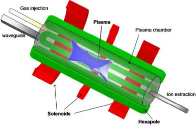
Simple mirror represents one of the more simple magnetic systems enabling plasma confinement. These magnetic structures are stable by the point of view of a single particle approach, however, a MHD approach demonstrates that different instabilities can arise in the central region of the mirror, lead-ing to a plasma flux in perpendicular direction with respect to the mirror axis [2]. The more efficient magnetic system able to guarantee the plasma confinement is the so called minimum B structure[9]. In such configura-tion, the magnetic field increases in every direction away from the plasma boundary, and there not exist any region where the magnetic field goes to zero inside the plasma. The scattering of the particles in the loss cone is essentially due to the Spitzer collisions. Such a configuration can be ob-tained as a superposition of two different magnetic fields: one created by two solenoids (simple mirror), and the other created by six conductors sur-rounding the plasma chamber (an hexapole), as shown in figure 1.6.3. In this way the magnetic field increases in every direction going from the plasma. Ioffe demonstrated [9] on B-min configurations that the confinement times are one hundred times higher than simple mirrors. Hence the B-minimum structure represents the fundamental magnetic configuration characterizing the ECRIS. Such a structure enables them to increase ion lifetime and to generate highly charged ion currents. A complete description of the parti-cle motion and of the ion confinement in a B-minimum structure is beyond the scopes of the present work. A more detailed analysis can be found in reference [10].
Figure 1.6.3: Magnetic system (a) and magnetic field structure (b) obtained by the superposition of the field produced by two solenoids and an hexapole (minimum-B field).
Waves in plasmas
The study of wave propagation has an extraordinary importance in plasma physics. MDIS and ECRIS plasmas, in facts, are generated and sustained by means of the interaction with E.M. waves. Furthermore, electrostatic waves (E.S.) can be generated within plasmas, able to strongly influence the Electron Energy Distribution Function (EEDF) or modifiy the diffusion rates of the species. Plasma Waves are always associated with a time and space varying electric field, and the propagation properties of such fields are determined by the dielectric properties of the medium, which in turn depend on applied magneto-static or electrostatic fields. A plasma may be both inhomogeneous and anisotropic, and this affects its dielectric proper-ties. The anisotropy can be easily induced by a magneto-static field, if any. MDIS and ECRIS plasmas, for example, are anisotropic media by the point of view of electromagnetic wave propagation. The first part of the chapter will be dedicated to the interaction between E.M waves and plasmas, with particular attention to the mechanisms which take to the Electron Cyclotron Resonance in ECRIS and to the microwaves energy absorption in MDIS. The second part will be dedicated to an introduction to E.S. waves and to the study of the E.M waves to E.S. waves coupling. Finally the last part of the chapter will be dedicated to the complete characterization of the Electro-static Bernstein waves (EBW). EBW, in facts, enables us to obtain electron densities and temperatures much higher than the usual E.C.R heating, in such a way increasing the quality factor of the ion sources.
ther details). The E.M. waves propagate in the plasma with phase velocity of 107 − 108m/s, values much higher than the particles thermal velocity
(103 − 105m/s), except for the restricted regions where the waves exhibit
resonances1; therefore, the cold plasma model is a useful approximation to determine the dispersion relation of the E.M wave in a magnetized plasma. In the following only the propagating electric field on E.M. wave will be con-sidered. The module of magnetic force due to the influence of the magnetic field of the wave, in facts, is [3]:
Fm=
v c
√
ϵrqE (2.1.1)
Thus, for particles velocity v << c the magnetic field of the wave can be neglected. This approximation is totally valid in the case of MDIS, whereas in ECRIS only a little part of hot electrons (see section 1.2.3) can reach relativistic energies, then being influenced by the magnetic field of the wave. For the scope of this section the magnetic effect can be neglected.
ECRIS and MDIS operative frequencies range between 2.45 GHz and some tens of GHz. At so high frequency ions are unsensitive to the electric field because of their high inertia, and their contribution in wave propagation can be neglected.
2.1.1 E.M. waves in a cold-unmagnetized plasma
In absence of a magnetic field, plasma is an isotropic medium. This means that the constitutive parameters assume the simple form of multiplicative
1As it will be shown in section 2.1.3, at the resonance the phase velocity of the E.M
constants. The fluid equation (1.3.9), in absence of magnetic field and in the cold plasma approximation becomes:
∂⃗v
∂t = q ⃗E (2.1.2)
Assuming that both electric field and velocity are varying in time as eiωt,
following the direction of the electric field, it can be easily shown that the dielectric constant is [3]: ϵ = ϵ0 1 −ω 2 p ω2 (2.1.3) where ωpis the plasma frequency and represents the natural oscillation
frequency of an electron in a plasma (see section 2.4). The plasma frequency is proportional to the square root of the electron density:
ωp =
ne2
ϵ0me
(2.1.4) As ϵ is defined positive, from equation (2.1.4) it follows that:
1 −ω 2 p ω2 ≥ 0 → ω2 > ωp2 (2.1.5) this means that electromagnetic waves with frequencies lower than ωpcannot
propagate into the plasma. As a consequence in homogeneous and non magnetized plasmas the density cannot exceed the so called cutoff density given by: ncutof f = 4π2 mϵ0 e2 f 2 p (2.1.6)
An overdense (i.e. above the cutoff) plasma would totally reflect the incoming (feeding) wave, so that the plasma would automatically adjust its own density to contemporary allow the maximum production with trans-parency for wave propagation. The cutoff density is consequently the main limitation of the plasmas generated by means of E.M waves. Plasmas hav-ing a density larger than the cut-off density, i.e. ne > ncutof f, are usually
named overdense. When this condition is not satisfied, i.e. ne < ncutof f,
the plasma is named underdense. The dispersion relation for waves in unmagnetized plasma is [2]:
Except for values close to ωp, the penetration depth δ is of the order of
1 cm., i.e. small compared to most ECRIS plasma.
2.1.2 E.M. waves in a cold-Magnetized plasma
If we apply a magneto-static field to the plasma, then it will become an anisotropic medium for the electromagnetic waves propagation. Necessarily, the dielectric constant will transform in a tensor (¯¯ϵ), as the field propagation will depend on the direction of propagation of the wave with respect to the external magnetic field.
Let’s assume, without losing in generality, ⃗B directed along the z axis, so that it can be written as ⃗B = B0z. It is possible to consider the plasma asˆ
a dielectric with internal current ⃗j. As a consequence, the fourth Maxwell equation can be written as:
⃗ ∇ × ⃗B = µ0 ⃗j + ϵ0 ∂ ⃗E ∂t = µ0 ∂ ⃗D ∂t (2.1.10)
By assuming a eiωt dependence for all plasma motions and by defining a conductivity tensor ¯σ, by the relation ⃗j = ¯¯ σ · ⃗¯ E, it is possible to obtain the relation between ⃗D and ⃗E:
⃗ D = ϵ0 ¯ ¯ I + i ϵ0ω ¯ ¯ σ · ⃗E (2.1.11)
Where ¯I is the identity tensor. Remembering that, in a general way, ⃗¯ D is linked to ⃗E by the relation:
⃗
Then the effective dielectric constant of the plasma is the tensor: ¯ ¯ ϵ = ϵ0 ¯ ¯ I + i ϵ0ω ¯ ¯ σ (2.1.13) To evaluate ¯σ, we use the fluid equation (1.3.9).¯ By neglecting the collisional effects and the pressure terms, according to the cold plasma ap-proximation, one obtains:
mi
∂⃗v
∂t = e ⃗E + ⃗vs× ⃗B
(2.1.14) This vectorial equation is equivalent to a system of three scalar equations, whose solution gives the relation between ⃗v and the electric field of the wave
⃗
E, therefore between ⃗j and ⃗E, since ⃗j = ne⃗v and also ⃗j = ¯σ ⃗¯E. For sake of brevity, the algebraic passages will be omitted and only the final value of the dielectric tensor ¯ϵ, obtainable from ¯¯ σ by means of relation (2.1.13), is¯ shown: ¯ ¯ ϵ = ϵ0 S −iD 0 iD S 0 0 0 P ≡ ϵ0ϵ¯¯r (2.1.15)
where S, D and P are respectively [1]
S ≡ 1 −ω 2 p ω2 1 1 − ωc (2.1.16) D ≡ −ω 2 p ω2 ωc ω 1 1 − ωc (2.1.17) P ≡ 1 −ω 2 p ω2 (2.1.18)
We can derive the wave equation by taking the curl of the Maxwell equation ⃗∇ × ⃗E = −∂ ⃗B
∂t and remembering equations (2.1.10) and (2.1.12) we obtain: ⃗ ∇ × ⃗∇ × ⃗E = −µ0ϵ0ϵ¯¯r· ∂2E⃗ ∂t2 = − 1 c2ϵ¯¯r· ∂2E⃗ ∂t2 (2.1.19)
Finally, by assuming an ei⃗k·⃗r spatial dependence of the electric field, and by introducing the vectorial index of refraction, we can write:
iD S − N 0 N2cos θ sin θ 0 P − N2sin2θ
Ey
Ez
= 0 (2.1.22) Equation (2.1.22) is a set of three simultaneous, homogeneous equations. The condition for the existence of a solution is that the determinant of the coefficient matrix vanishes. This condition, finally, gives out the relation dispersion for E.M waves in plasmas:
S sin2θ + P cos2θ N4+RL sin2θ + SP (1 + cos2θ) N2+ P RL = 0
(2.1.23) where, for sake of simplicity, we defined R = S +D and L = S −D. Equation (2.1.23) contains all the information about the propagation of the waves in magnetized plasma. it has two solutions:
No,x2 (θ) = 1 − 2X(1 − X)
2(1 − X) − Y2sin2θ ±
Y4sin4θ + 4Y2(1 − X)2cos2θ
(2.1.24) Hence for a given arbitrary direction, defined by θ, we have two waves char-acterized by different index of refraction. No(θ) is called ordinary wave, whereas Nx(θ) is named extraordinary wave. Here we have introduced two important parameters, X and Y , which will be very useful to simplify the mathematical notation:
X = ω 2 p ω2 ∝ ne Y = ωc ω ∝ B0 (2.1.25)
X is the parametric electron density, proportional to ne, whereas Y is the
2.1.3 Cutoffs and resonances
By means of equation (2.1.24) it is possible to determine the wave’s propa-gation properties as a function of the angle θ, of the electron density neand
of the magnetic field B0. By definition, the index of refraction N is positive,
so that the wave can propagate in the medium only if N > 0. In general we can have four different cases:
• N > 0 Propagation region: The wave propagates in the medium with phase velocity given by c/N ;
• N < 0 Stop-band region: The wave can not propagate; • N = 0 Cut-off : The wave is reflected;
• N → ∞ Resonance: The wave is absorbed by the medium.
According to equation (2.1.24), cutoffs can be found by setting N = 0. So they occur only when is verified the condition P RL = 0, i.e. when:
P = 0 or R = 0 or L = 0 (2.1.26)
It is very important to note that condition (2.1.26) does not depend on θ. Thus cutoffs does not depend on the angle of propagation θ. From (2.1.26), thus we obtain the three cutoffs of E.M. in magnetized plasmas expressed as a function of plasma parameters:
1. P = 0 ⇒ ω = ωp or X = 1: as in unmagnetized plasmas, ω = ωp is
a cutoff condition also in magnetized plasmas. This cutoff is usually named O cutoff ; 2. R = 0 ⇒ ω = ωR = 12 ω2 c + 4ωp2+ ωc or Y = 1 − X: this cutoff is named upper cutoff frequency or R cutoff, occurring at frequency above both ωp and ωc;
3. L = 0 ⇒ ω = ωL = 12 ω2 c + 4ω2p− ωc or Y = X − 1: this cutoff is named lower cutoff frequency or L cutoff, placed below ωp;
Ordinary waves are reflected when ωRF = ωp i.e at O cutoff.
Extraor-dinary waves are unaffected by this cutoff and reflected at R and L cutoffs (they are not reflected at O cutoff, being, N2|X=1̸= 0). Resonances can be
Figure 2.1.1: Resonance cones in a magnetized plasma. The wave encounters a resonance only on the surface of the cone of angle θc, where the relation tan2θr=
−P
S is satisfied.
found by imposing the condition N → ∞ in equation (2.1.23), which imply that the coefficient of the term of larger order (N4) must go to zero2:
S sin2θ + P cos2θ = 0 → tan2θr= −
P
S (2.1.27)
The resonance angle θr can be written as a function of the plasma
pa-rameters as it follows:
cos2θr=
X + Y2− 1
XY2 (2.1.28)
If the electron density and the applied magnetic field are almost con-stant3, thus the resonance can occur only on the surface of a cone, named resonant cone [19], whose axis is aligned with the external magnetic field B0z and with aperture angle θˆ r, as displayed in figure 2.1.1. This cone
corresponds to conical surfaces in the real space.
2
to verify this it is sufficient to we set M = 1/N4 in equation (2.1.23) and look for M=0 solution. When M → 0, then N → 0.
3
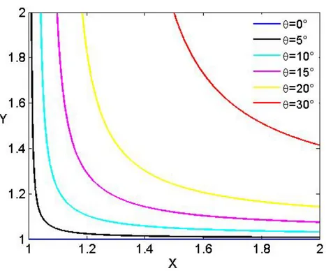
The conditions for establishing of the resonances, thus, depend on the di-rection of wave propagation. By setting the denominator of equation (2.1.24) equal to zero it is possible to verify that only the extraordinary wave can have resonances. Equation (2.1.28) enable us to calculate the value of X and Y needed to have a resonance at the angle θr. For the special angle θ = 0◦
the resonance takes place for each value of X when Y = 1 i.e ω = ωRF = ωc.
In this case the microwave frequency is equal to the Larmor frequency, hence the wave is in resonance with the cyclotron motion of the electrons. This res-onance is of primary importance for ECRIS and MDIS and takes the name of Electron Cyclotron Resonance. In plasma physics, the extraordinary wave propagating with θ=0 is named R wave. For the special angle θ = 90◦ the resonance occurs when X + Y2− 1 = 0 i.e:
ωRF = ωU HR=
ω2
c + ωp2 (2.1.29)
This resonance is named Upper Hybrid Resonance (UHR), and the wave propagating exactly across ⃗B0 (θ = 90
◦
) is named X wave.
The resonance condition implies that X and Y parameters lie on a parabola, as shown in figure 2.1.2. At this frequency the electrons are subjected to the cyclotron motion at frequency ωc and to the plasma oscillation, having
frequency ωp. The combination of the two motions turns the trajectory
into ellipses which are covered with resulting frequency ωU H =
ω2
p+ ω2c.
When ωRF = ωU HR the energy of the microwave can be transferred to
plasma waves. For a generic angle θ, the resonances of the extraordinary wave are placed in the X − Y plane lying between ECR and UHR. It is important to notice that the resonance curves lie in the plane X, Y ≤ 1, i.e. when ω ≤ ωcand ω ≤ ωp. Only when the incidence angle is exactly zero the
resonance (ECR) can occur even at density larger than the cutoff density. Because this effect is found for just a single value of the angle θ (i.e. it represents a sort of singularity). The existence of an ”overdense resonance” can be viewed more like a formal consequence of a mathematical treatment that a real physical process.
Figure 2.1.2: Corresponding values of X and Y parameters satisfying resonance conditions of the Extraordinary waves propagating for different propagation angles θ.
Figure 2.1.3: Resonances of the Ordinary waves propagating for different angle propagation angles θ.
The resonances of the Ordinary waves can be found easily by looking at the zeroes of equation (2.1.24). It is easy to see that these solutions correspond to the ones of equation (2.1.28) placed in the X, Y ≥ 1 region of the X-Y plane4, as shown in figure 2.1.3. These resonances, however, are placed in a forbidden region for ordinary waves, i.e. over the O cutoff X=1; therefore such resonances could be reached only by wave tunneling through the O cutoff. In case of incidence angle θ = 0◦, the ordinary wave is named L wave, and it encounters a resonance for Y=1. When θ increases, hyperbole shaped resonances move toward larger values of X and Y.
As we have seen above, a conventional nomenclature is normally adopted in plasma physics to label waves propagating at certain angles, in particular at 0◦ and 90◦. Ordinary waves propagating along or across the magnetic
4
In a more general picture, taking into account also ion motion, ordinary wave can be absorbed by ions at Ion Cyclotron Resonance (ωi= ωRF), while at the Lower Hybrid
Figure 2.1.4: Scheme of the wave propagation in anisotropic plasmas. According to the mutual orientation of ⃗k, ⃗E and ⃗B, the last being the magnetostatic field, the waves have different characteristics and are named R, L, O and X [10]. See also figure 2.1.6.
field are respectively named O wave and L waves. As we introduced previ-ously, Extraordinary waves propagating along or across the magnetic field are respectively named R wave and X waves. A scheme of the four type of waves is shown in figure 2.1.4, whereas in table 2.1.5 the respective refrac-tion indexes, obtainable from equarefrac-tion (2.1.24) are displayed. For a more detailed treatment of these issues we refer to the next sections.
Figure 2.1.5: Cutoffs and resonances of the waves propagating in a magnetized plasma considering θ = 0, θ = 90◦ directions.
It can be useful to study the polarization of the waves in a magnetized plasma. From the middle line of equation (2.1.22) it is possible to calcu-late the relation between Ex and Ey, that is the polarization in the plane
perpendicular to ⃗B0: iEx Ey = N 2− S D (2.1.30)
From this relation it follows that the waves are linearly polarized at the resonance (N2 = ∞ → Ey = 0) and circularly polarized at cutoff (N2= 0 ,
R = 0 or L = 0 → Ex± Ey). Furthermore, following [3], it comes out that
the ordinary waves are left-hand polarized, whereas extraordinary waves are right-hand polarized. A sketch showing the orientation of the electric field with respect to the magnetostatic field is shown in figure 2.1.6.
Figure 2.1.6: Diagram showing the possible orientations of the electric field with respect to the magnetostatic field, along with the possible waves polarizations [2].
Because of their polarization, electric field of the R wave rotates in the same direction and versus of the gyrating electrons in a magnetic field. When the frequency of the injected microwave ωRF matches the cyclotron
fre-quency ωc, then electrons see a constant field leading to resonant energy
absorption. If the electrons gain enough energy, they are able to ionize the neutrals of the nascent plasma. It is really important to note that in a collisionless plasma, the ECR is the only physical mechanism al-lowing the direct energy transfer from E.M wave to electrons. The mechanism of the resonant electron acceleration can be easily demonstrated by looking to the solution of the equation of motion (2.1.14) for an harmonic E.M field in a magnetized plasma acting on a free electron:


![Figure 2.1.7: Trivelpiece-Gould dispersion curves for electrostatic electron waves in a magnetized plasma [21] in ω c > ω p and ω c < ω p plasma regions](https://thumb-eu.123doks.com/thumbv2/123dokorg/4531489.35341/56.892.347.617.327.776/figure-trivelpiece-dispersion-curves-electrostatic-electron-magnetized-regions.webp)


![Figure 3.3.6: R wave electric field vector rotations and electron gyrations in ECR (bottom), off-ECR (middle), and with B ¿ BECR [2].](https://thumb-eu.123doks.com/thumbv2/123dokorg/4531489.35341/95.892.266.555.188.613/figure-electric-field-vector-rotations-electron-gyrations-middle.webp)
