UNIVERSITÀ DEGLI STUDI DELLA TUSCIA DI VITERBO
DIPARTIMENTO DI SCIENZE ECOLOGICHE E BIOLOGICHE
CORSO DI DOTTORATO DI RICERCA IN
ECOLOGIA E GESTIONE DELLE RISORSE BIOLOGICHE XXVII CICLO.
P
LEISTOCENE EVOLUTIONARY HISTORY AND
CONSERVATION OF MOUNTAIN SPECIES WITHIN
M
EDITERRANEAN PENINSULAS
:
INSIGHT FROM THE
A
LPINE NEWT IN THE
A
PENNINE CHAIN
(BIO/07)
TESI DI DOTTORATO DI: DOTT. ANDREA CHIOCCHIO
COORDINATORE DEL CORSO TUTORE
PROF. DANIELE CANESTRELLI PROF. DANIELE CANESTRELLI
DATA DELLA DISCUSSIONE
17/06/2016
2
I
NDEXChapter 1 – Introduction ...3
1.1 Background and aims of the research ...3
1.2 The study species Ichthyosaura alpestris ...7
Chapter 2 – Genetic structure and evolutionary history of
Ichthyosaura alpestris within Apennine peninsula ...9
2.1 Introduction ...10
2.2 Materials and methods ...13
2.3 Results ...19
2.4 Discussion ...24
2.5 Tables and Figures ...29
Chapter 3 – Geographic distribution of the chytrid pathogen
Batrachochytrium dendrobatidis among mountain amphibians along the
Italian peninsula ...41
3.1 Introduction ...42
3.2 Materials and methods ...44
3.3 Results ...46
3.4 Discussion ...47
3.5 Tables and Figures ...49
Chapter 4 – Discussion ...51
Appendix ...55
3
1.
I
NTRODUCTION1.1 BACKGROUND AND AIMS OF THE RESEARCH
Investigations of species genetic structure have shown that genetic diversity is usually distributed unevenly among populations (Hewitt, 2004). Historical processes linked to palaeoecological changes and on-going processes linked to population responses at the strong human impact on the environment must both be considered among the main causes of this unevenness (Hewitt, 2004; Yannic et al, 2014).
Among historical processes, a leading role was played by the Pliocene climatic revolutions and above all, by the Pleistocene glacial cycles (Hewitt, 1996, 1999, 2000, 2011a,b). Such climatic variations have deeply affected species distribution, repeatedly fragmenting the populations during climatically unsuitable phases, and triggering demographic and adaptive responses, which resulted in genetic population divergence (Hewitt, 1996, 2000; Dynesius & Jansson, 2000; Davis & Shaw, 2001).Many species have survived the adverse conditions of Pleistocene glacials in relatively suitable areas named refugia (Bennet & Provan, 2008; Stewart et al., 2010). Several studies have highlighted that pleistocenic refugial areas were not only the richest in species biodiversity, but are often areas that retain the most intraspecific biodiversity (Petit et al, 2003). Some researchers have suggested that long-term stability within refugia may have promoted the accumulation of genetic diversity over time (Carnaval et al., 2009; Abellan & Svennig, 2014). However, the main assumption of this hypothesis is the maintaining over time, a population size large enough to avoid the effects of genetic drift and inbreeding, which negatively affect the levels of genetic diversity (Keller & Waller, 2002; Charlesworth, 2003). Nevertheless, such a condition is difficult to realize in geographically heterogeneous refugia such as mountain refugia (Knowles & Richards, 2005). Moreover, the numerous cases where many differentiated lineages were found within a single refugial area suggest the engagement of more complex microevolutionary processes, possibly linked to a putative fragmentation within the refugium (Stewart et al., 2010).
Within fragmented areas, secondary contact among previously isolated populations may have carried out a leading role in triggering the microevolutionary processes that affect the genetic diversity of populations (Taberlet, 1998; Hewitt, 2011b). Secondary contact promotes different mechanisms according to the duration of contact and genetic
4
differentiation previously gained by populations (Barton & Gale, 1993; Burke & Arnolds, 2001). On one hand, if genetic differentiation is high, secondary contact may promote the evolution of reproductive isolation, and then speciation (Coyne & Orr, 1997); on the other hand, if genetic differentiation is low or moderate, secondary contact allows the admixing of gene pools, causing reinvigoration of populations (Crow, 1948; Barton, 2001). In the latter case, secondary contact drives populations to gain size and heterozygosis, thus improving their health status (Ingvarsoon & Whitlock, 2000; Whitlock et al, 2000; Chapman et al, 2009). Secondary contact of short duration, which is not long enough to completely admix the gene pools of populations, may even allow introgression of private genes from one population to another (Hewitt, 2011b). Traces of palaeo-introgression may provide useful information about past gene flow between two genetic lineages (McKinnon
et al, 2004). Such mechanisms can be considered not only as an explanation for high levels
of genetic diversity, but also as responsible for long-term survival of populations.
Several evidences regarding the role of fragmentation and secondary contact in increasing genetic variations within refugia arise from phylogeographic studies in Southern European peninsulas (Taberlet, 1998; Hewitt, 2011a,b). These peninsulas are hotspots of biodiversity at both the inter- and intra-specific level, and were refugia for several Palaearctic species during the Pleistocene glacial phases, when the rest of Europe was covered by ice and tundra (Hewitt, 2004, 2011a; Weiss & Ferrand, 2007; Feliner, 2011). Many of these studies have identified several genetic lineages strongly differentiated within a single refugium, in some cases sufficient to be split in two separate species (e.g.
Salamandrina terdigitata e S. persicillata, Canestrelli et al., 2006c). A variation so high,
has suggested that these areas could be composed of more sub-refugia, and the high genetic diversity might be a result of repeated contraction and expansion of populations, which resulted in repeated isolation and secondary contact among their gene pools (Gomez & Lunt, 2007). Three evidences could confirm that this mechanism, and not stability, should be responsible for the observed pattern of genetic variation: areas with the highest diversity are also most affected by palaeoclimatic or palaeogeographic changes; the highest levels of heterozygosis are not within refugia, but in the contact area among the expanding lineages; the areas with the most healthy populations are the ones affected by this mechanism. Some case studies on the Apennine peninsula can be considered to summarise these evidences: Talpa romana (Canestrelli et. al., 2010), Rana italica (Canestrelli et al., 2008), and Bombina pachypus (Canestrelli et al., 2006b). All three cases highlight the leading role of admixture among genetic lineages differentiated inside different
sub-5
refugia, in realizing the hotspot of intraspecific genetic diversity. Of particular relevance is the case of B. pachypus: this species shows strong decline across all Apennine peninsula, caused by a synergistic effect of on-going climate change and infection from the chytrid fungus Batrachochytrium dendrobatidis. The only populations that do not show any sign of decline are the calabrian populations, which have the highest level of genetic diversity and which resulted from the admixing of more lineages from different sub-refugia (Canestrelli et al., 2013). This case again confirms the leading role of genetic diversity in conferring the evolutionary potential indispensable to survive in natural stress. Such evidences support the hypothesis that genetic diversity inside refugia is closely linked to the dynamics of fragmentation, differentiation, and secondary contact, and that genetic diversity may have played an active role in the long-term survival of populations, rather than being a by-product of persistence.
Most evidences on evolutionary dynamics involved in southern European peninsular refugia come from studies on temperate species (Hewitt, 2011a). However, many mountain chains that run across these peninsulas have also provided refugia to a number of cold-adapted species, which represent a large portion of the biodiversity in these areas (Schmitt, 2009; Medail & Diadema, 2009; Vogiatzakis, 2012). Mountain refugia have a strongly fragmented distribution, and they were highly instable, since many of them were covered with ice during the glacial phases, forcing the cold-adapted populations to move away to the peripheral areas (Schönswetter et al., 2005; Schmitt et al., 2006; Varga & Schmitt, 2008; Holderegger & Thiel-Egenter, 2009; Schmitt, 2009; Garrick, 2011). Both habitat discontinuity and instability of their Pleisocene refugia are useful prerequisites of mountain species to study the role of fragmentation and secondary contact in shaping the distribution of genetic diversity among the populations inside refugia.
Understanding the distribution of genetic diversity among populations of cold-adapted species could be fundamental to direct conservation planning for species that are threatened by on-going climate changes (Parmesan, 2006). It has been observed that climate change is altering mountain habitats, and severe population decline of many cold-adapted species caused by loss of habitat suitability have been reported in the last few years (Diaz et al., 2006). Moreover, climate changes may disrupt the equilibrium of some ecosystem interactions such as host-pathogen interactions, resulting in increased risk of extinction for several species (Harvell et al., 2002). Association among amphibian decline, climate changes, and the outbreaks of an infectious disease, chytridiomycosis, was reported in the last decade (Pounds et al., 2006). Chytridiomycosis, caused by the chytrid fungus B.
6 dendrobatidis, is an infectious disease affecting the keratinized epidermal cells of its
amphibian hosts, and is currently among the main causes of amphibian decline (Berger et
al., 1998; Daszak et al., 1999; 2003; Fisher et al., 2009; Kilpatrick et al., 2010). In the
above-mentioned decline of B. pachypus in the Apennine peninsula, different responses of populations to the pathogen have been observed, along with a delay between the presence of the pathogen in the populations and the signs of decline. Such a temporally and spatially heterogeneous pattern was attributed to the differing capacities of populations to respond to stress, linked to their differing levels of genetic variability and evolutionary potential. Moreover, altitude seems to be positively related to the severity of this disease, since the most severe mass mortalities have been observed in mountain species (Berger et al., 1998; Fellers et al., 2001; Bosch et al., 2001). In Europe, a strong association was found between altitude and the mass mortality of three common species: Alytes obstetricans, Salamandra
salamandra, and Bufo bufo (Bosch et al., 2001; Bosch & Martínez-Solano, 2006, Walker et al., 2010). This stronger vulnerability of high-altitude populations to both climate
changes and chytrid disease, and the possible association between this vulnerability and genetic diversity suggest that cold-adapted amphibians could be used to study the relationship between evolutionary history, genetic diversity, and the evolutionary potential of populations.
In the present study, we evaluate the role of Pleistocene glaciations in moulding the genetic structure of a cold-adapted amphibian living in the Apennine peninsula,
Ichthyosaura alpestris. The main aim is to evaluate the hypothesis that even in
cold-adapted species, fragmentation of refugia and secondary contact among differentiated populations could have played a leading role in shaping the genetic variation within the peninsular refugia. This is the first study on Apennine cold-adapted species with exhaustive sampling across the peninsular range, using a multi-locus dataset. We assess the genetic variation in both mitochondrial and nuclear markers with the following objectives: to analyse the genetic structure of Apennine populations; identify the evolutionary and biogeographic processes involved; to evaluate the role of fragmentation and secondary contact in distribution of genetic diversity; and to evaluate if differences in genetic diversity among populations may be related to population health and the capacity to respond to stress factors. Moreover, we use molecular diagnostic assays to test for the occurrence of chytrid fungus among the populations of I. alpestris and two other sympatric
7
mountain species, to assess any relationship between pathogen occurrence, altitude, and population decline.
1.2 THE STUDY SPECIES
I
CHTHYOSAURA ALPESTRISThe study species is the Alpine newt Ichthyosaura alpestris (Laurenti, 1768), a cold-adapted amphibian of the family Salamandridae. This species is widespread throughout much of Europe, ranging from the French Atlantic coastline to the north of Denmark and eastwards to the Ukrainian Carpathians, Romania, and Bulgaria; it is widely distributed in the Balkans and in the northern Apennines, whereas isolated populations are present in southern Italy and northern Spain (Sillero et al., 2014). Within the Apennine peninsula, there are two geographically, morphologically, and genetically differentiated subspecies: I.
alpestris apuana (Bonaparte, 1839), ranging from the north-western to central Apennines
and I. alpestris inexpectata (Dubois e Breuil, 1983), which is present as a few isolated populations in the southern Apennine (Sindaco et al., 2006). Apennine populations have shown to be a distinct genetic lineage with respect to the Alps and European populations, and their isolation was estimated to be of the lower Pliocene origin (Recuero et al., 2014). The habitats of the Alpine newt in the Apennine peninsula include permanent and semi-permanent ponds as well as small lakes between 800 and 1800 m s.l.m., even though several populations can be found in the wet hills of the Ligurian Apennines below 500 m s.l.m (Ambrogio & Gilli, 1998).
Among European newts, I. alpestris is the most linked to water, and several adults can be found within ponds all around the year. Most of the Apennine populations show a high percentage of pedomorphic individuals, which are sexually reproductive individuals that maintain morphological and physiological features of larva. The relative roles of genes and the environment in determining pedomorphism in I. alpestris is unknown but it has been suggested that pedomorphism could be an adaptation to the unstable climatic conditions of Apennine mountains habitats. Pedomorphism negatively affects dispersal, by reducing the number of individuals that leave native ponds (Denoel et al., 2001, Denoel, 2003). The breeding season is between March and July, according to altitude and latitude of the reproductive sites, but a second breeding season can be observed in autumn; metamorphosis typically occurs before winter or in the subsequent spring, and sexual maturity is achieved around the second and fourth year. The Alpine newt feeds on little
8
invertebrates, and it is preyed upon by insects (Odonate, Ditiscidae and aquatic Eteroptera), as well as by bigger newts, fish, or aquatic birds when present (Ambrogio & Gilli, 1998).
Apennine populations of I. alpestris are considered as “Near Threatened” by the IUCN, except for the Southernmost isolated populations, which are considered as “Endangered” (Rondinini et al., 2013). The main causes of extinction include climate changes, pollution, habitat degradation or loss, habitat fragmentation and population isolation, and introduction of fishes. Evidence of individual mortality or population decline attributable to chytridiomycosis has not been reported for the Apennine peninsula until now.
9
2.
G
ENETIC STRUCTURE ANDE
VOLUTIONARY HISTORY OFI
CHTHYOSAURA ALPESTRIS WITHINA
PENNINE PENINSULAABSTRACT
Southern European peninsulas provided refugia for several species during Quaternary climatic oscillations, and several phylogeographic studies have investigated the evolutionary processes involved. The view of these refugia as static and stable has been changing since even more studies are revealing many intraspecific genetic lineages within them, highlighting the role of refugia sub-structuring in enhancing genetic diversity. Although mountains harbour a great part of biodiversity in these peninsulas, most of the study was focalized on temperate species, whereas the evolutionary dynamics involving the cold-adapted species are underinvestigated. Here, we use a bayesian phylogeographic approach, coupled with a species distribution model to investigate the genetic structure and the evolutionary history of the cold-adapted amphibian, Ichthyosaura alpestris within the Apennine peninsula. Both mitochondrial and nuclear markers identified three distinct lineages, whose divergence dates back to the Early and Middle Pleistocene. Two of these lineages form a secondary contact zone in the Ligurian Apennine, which corresponds to one of the main biogeographic discontinuities of the peninsula. Our spatiotemporal phylogeographic reconstruction identified the Riss glacial as the period of expansion and contact for these lineages. Nevertheless, SDM analysis indicated the contact zone as a suitable region during both the last interglacial and the last glacial, conditions that may have prolonged lineage admixture until now. Our results confirm the role of southern European peninsulas as multiple refugia during the Pleistocene for cold-adapted species as well, and suggest that repeated cycles of allopatric fragmentation followed by secondary admixture may have been a common process in forming hotspots of intraspecific diversity within these peninsulas.
KEY WORDS: genetic diversity, bayesian phylogeography, Pleistocene refugia, Apennine peninsula, cold-adapted species, Icthyosaura alpestris
10
2.1 INTRODUCTION
Southern European peninsulas are hotspots of biodiversity at both the species and genetic levels, and the processes generating this richness have always attracted the interest of biogeographers and evolutionary biologists (de Lattin, 1967; Hewitt, 1996, 2011; Taberlet et al., 1998; Weiss & Ferrand, 2007). It is now established that Pleistocene climatic oscillations have influenced the distribution of biodiversity in these areas, causing shifts in species ranges and triggering evolutionary processes that have moulded species’ genetic structures (Comes & Kadereit, 1998; Hewitt, 2000; Hofreiter & Stewart, 2009; Feliner, 2011). During glacial maxima, several species took refuge in southern European peninsulas, and vicariance events among isolated populations promoted differentiation and speciation (Taberlet et al., 1998; Hewitt, 2001; Schmitt, 2007; Bennett & Provan, 2008). Genetic diversity was often increased by further sub-structuring within these refugia, where populations were repeatedly fragmented and reshuffled by cyclic range contractions and expansions (Petit et al.,2003; Hampe e Petit, 2005; Gomez & Lunt, 2007; Canestrelli
et al., 2010; Stewart et al., 2010). The strong habitat heterogeneity within these peninsulas,
where lowland, hilly and mountain habitats contain refugia for temperate as well as cold-adapted species, made them suitable as both glacial and interglacial refugia (Stewart et al., 2010). However, differences between the processes involved in glacial and interglacial refugia are not yet fully understood, and the phylogeographical investigation of these areas continues to be of great interest (Hewitt, 2011a).
Mountains play a key role in understanding species’ responses to past climate change in southern European peninsulas. They have had a strong impact on species genetic structure by acting as ecological barriers to temperate species during glacial periods as well as refugia for cold-adapted species during interglacial phases (Schmitt, 2009). Despite the fact that several Mediterranean refugia are located in mountainous areas (Medail & Diadema, 2009; Vogiatzakis, 2012), most attention has been paid to temperate species, and few phylogeographic studies have been conducted on cold-adapted species (Schönswetter
et al., 2005; Schmitt, 2009). However, because climatic events had different consequences
on cold-adapted species, investigating their evolutionary history is crucial in understanding the dynamics involved in species evolution during the Pleistocene (Louy et al., 2014). Indeed, mountain refugia are structurally highly discontinuous (Varga & Schmitt, 2008; Holderegger & Thiel-Egenter, 2009; Garrick, 2011), and cold-adapted populations
11
probably encountered stronger fragmentation during interglacial periods. However, because interglacial phases were shorter than glacial phases, populations isolated during interglagials should be less genetically differentiated than population isolated during glacial (Stewart et al., 2010; Garcia et al., 2011). Moreover, many interglacial refugia were unstable environments because they were covered by ice or were too dry for cold-adapted species during glacial culminations, forcing populations to move to peripheral areas (Schönswetter et al., 2005; Schmitt et al., 2006; Varga & Schmitt, 2008; Holderegger & Thiel-Egenter, 2009; Schmitt, 2009). Therefore, populations of cold-adapted species could have experienced strong environmental constraints, both during interglacial and glacial periods, with different time frames, refugial sites and recolonization routes that could have produced several unique evolutionary pathways.
Despite the Italian Peninsula was intensively studied phylogeographically, few studies have investigated the role of interglacial refugia in Pleistocene evolutionary history of cold-adapted species. Italian Peninsula is rich of mountainous areas, thanks to the presence of Apennines, a mid-to-high-altitude mountain chain, which span more than 1200 km in a NW-SE direction, surrounded by hilly and lowland regions, and climatically very heterogeneous. Their role as refugia has been recognized for both temperate and cold-adapted species (Hewitt, 2011a, and references therein). Nonetheless, phylogeographic studies on the Italian Peninsula have almost exclusively examined temperate species, investigating their dynamics within glacial refugia and the role that major mountain blocks played on shaping their genetic variation (eg. Fritz et al., 2005 ; Boheme et al., 2006; Canestrelli et al., 2006, 2008, 2010, 2012, 2014; Heuertz et al., 2006; Ursembacher et al., 2006; Maura et al., 2014). In contrast, the few phylogeographic studies on cold-adapted species that have been conducted have not investigated the fine-scale genetic structure of Apennine populations, making it difficult to reconstruct their Pleistocenic evolutionary history (eg. Castiglia et al., 2009; Stefani et al., 2012).
In this study, we investigated the genetic structure and evolutionary history of an Apennine cold-adapted amphibian, the Alpine newt Ichthyosaura alpestris (Laurenti, 1768). This species is widely distributed in central and Eastern Europe where it breeds in small lakes and semi-permanent ponds, while in the Apennines its distribution is fragmented and closely linked to mid- and high-altitude ponds (Sillero et al., 2014). Morphological, ecological and genetic evidences suggest that the Apennine populations of this species should be considered two distinct subspecies: I. a. apuana for northern and central Apennine populations, and I. a. inexpectata for the southernmost Calabrian
12
populations (Breuil, 1986; Ambrogio & Gilli, 1998; Lanza et al., 2007). Interestingly, the separation of the Apennine clade from other European clades (including the Alps) has been estimated to be of pre-Pleistocene origin, but very little information is available about the genetic structure of the Apennine clades, making the Alpine newt an excellent model with which to study the impact of Quaternary glaciations on the evolution of cold-adapted species.
Using information from mitochondrial and nuclear DNA sequences in combination with Bayesian phylogeographic analysis and ecological niche modelling, we (1) assessed how, and how much, Quaternary climatic oscillations influenced the evolutionary history of these populations; (2) localised putative Pleistocenic refugia in the Apennines for this cold-adapted species; and (3) evaluated biogeographical and microevolutionary pathways that drove their evolution during the Pleistocene.
13
2.2 MATERIALS AND METHODS
Sampling and laboratory procedures
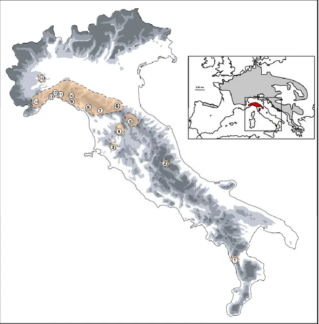
We collected 149 individuals of I. alpestris from 15 localities spanning its distribution in the Apennines; geographical references for sampling locations and sample sizes are shown in Table 1 and Fig. 1. Tissue samples were collected from tail tips after the newts had been anaesthetized by submersion in a 0.1% solution of MS222 (3-aminobenzoic acid ethyl ester). All of the individuals were then released at the respective collection site. Samples were stored in95% ethanol until subsequent analyses.
DNA extractions were performed by following the standard cetyltrimethyl-ammonium bromide (CTAB) protocol (Doyle & Doyle 1987). Two mitochondrial DNA (mtDNA) and three nuclear DNA (nDNA) fragments were amplified and sequenced. The mtDNA fragments consisted of one from the cytochrome B gene (CytB) and one from NADH dehydrogenase subunit 2 gene (ND2); the three nDNA fragments consisted of one from the fourth intron of the growth hormone gene (GH), one from the seventh intron of the β-fibrinogen gene (β-FIB) and one from the eleventh intron of the platelet-derived growth-factor receptor gene (PDGFR). The primers used and their sequences are presented in Table 2. Amplifications were performed in a 10-μLreaction volume containing MgCl2 (2 mM), four dNTPs (0.2 mM each), two primers (0.2 μM each), the enzyme Taq polymerase (0.5 U, Promega), its reaction buffer (1X, Promega) and 40–200 ng of DNA template. The polymerase chain reactions (PCRs) were conducted with an initial step at 95°C for 5 min, 32 cycles at 94°C for 1 min, annealing temperature and duration depending on fragment (see Table 2), 72°C for 1 min, followed by a single final step at 72°C for 5 min. To increase the specificity and yield of the β-FIB amplification, we used a nested PCR as in Sequeira at al. (2006), with slight modifications in the cycling conditions of the second PCR (26 cycles of 94°x30’’, 59°x30’’, 72°x45’’). Purification and sequencing of the PCR products were conducted on both strands by Macrogen Inc. (http://www.macrogen.com) using an ABI PRISM® 3730 sequencing system (Applied Biosystems). All of the sequences were deposited in GenBank (accession numbers: XXXX)
We also analysed variation at nine microsatellite loci (Copta1, Copta3, Copta8,
14
published protocols (Prunier et al., 2012, 2014). We chose a subset of available loci after the exclusion of those that exhibited reaction inconsistency in over 30% of samples. Forward primers were fluorescently labelled and PCR products were electrophoresed by Macrogen Inc. on an ABI 3730xl genetic analyser (Applied Biosystems) with a 400-HD size standard. The DNA fragments were analysed, and genotypic data were generated, using GeneMapper® 4.1. Micro-Checker 2.2.3 (Van Oosterhout et al., 2004) was used to test for null alleles and large-allele dropout influences. Because the tetranucleotide locus
Copta9 exhibits a dinucleotide variation in some populations, each allele was sequenced as
above; extraordinary allele sequences revealed a two-base-pair insertion in the flanking region of the simple sequence repeat (SSR). To use only true SSR polymorphisms in our analyses, the fragment length values of these alleles were corrected by subtracting 2.
Phylogenetic data analysis
Electropherograms were visually checked using FinchTV 1.4.0 (Geospiza Inc.) and sequences were aligned using Clustal X 2.0 (Larkin et al., 2007). Heterozygous nuclear sequences were phased using the PHASE method implemented in DnaSP 5.10 (Librado & Rozas, 2009), maintaining the default features; superimposed traces, produced by the direct sequencing of heterozygous indels, were resolved as suggested by Flot et al.(2006). For each nuclear gene, the probability of recombination was evaluated using the pairwise homoplasy index (PHI statistics, Bruen et al., 2006) in SplitsTree 4.13.1 (Huson & Bryant, 2006). All of the subsequent analyses were conducted using phased nuclear data, and indels were treated as missing data. Nucleotide variation was assessed using MEGA 6.0 (Tamura et al., 2013); haplotype and nucleotide diversity (Nei, 1987) were estimated using DnaSP 5.10.
Because no differences had been detected by a partition-homogeneity test (Farris et
al., 1994) implemented in PAUP* 4.0B10 (Swofford, 2003), the two mtDNA fragments
were combined into a unique haplotype using Concatenator 1.1.0 (Pina-Martins & Paulo, 2008). All of the subsequent analyses were conducted on the combined dataset.
Phylogenetic relationships between the mtDNA haplotypes were inferred using a maximum likelihood algorithm in PhyML 3.10 (Guindon et al., 2010). We used the default settings in PhyML for all of the parameters except for the type of tree improvement, choosing the SPR & NNI algorithm, and for the substitution model, using the Bayesian information criterion (BIC) best-fit model of evolution (HKY) selected by jModelTest
15
2.1.3 (Darriba et al., 2012); the robustness of the inferred tree was assessed using the non-parametric bootstrap method with 1000 replicates. The estimated tree topology was then converted into haplotype genealogy using Haplotype Viewer software (Salzburger et al., 2011). Genealogical relationships between the mtDNA haplotypes were investigated using a statistical parsimony approach in TCS 1.21 (Clement et al., 2000), with a 95% cut-off criterion for a parsimonious connection. The statistical parsimony approach was also used to investigate genealogical relationships between haplotypes for each nuclear fragment. MEGA 6.0 was used to compute the net sequence divergence among the haplogroups.
Divergence time estimations
The Bayesian procedure implemented in BEAST 1.8.1 (Drummond et al., 2012) was conducted in order to estimate the divergence time across lineages and the pattern of spatial diffusion. For these analyses we only used the mtDNA dataset, because it had exhibited much more variation than the nuclear sequence dataset. PartitionFinder 1.1 (Lanfear et al., 2012) was used to select the optimal partitioning strategy and substitution models for each partition, using linked branch length options and forcing the software to choose only among the models implemented in BEAST. Using BIC, the best scheme was the same for both genes: HKY for the first position, HKY for the second position and TrN93 for the third position. This partition scheme was used for all subsequent analyses.
We first estimated the divergence time between the haplotypes. A Bayesian skyline plot was chosen as a coalescent tree prior (Drummond et al., 2005). The molecular clock was calibrated by setting a normal prior for the treeModel.rootHeight parameter with a mean of 2.1 million years (standard deviation of 0.45), followingthe estimate of the most common ancestor of I. a. apuana in Recuero et al. (2014). This estimate was generated by a Bayesian analysis of divergence time among the main I. alpestris lineages using datation of the first Triturus fossil to calibrate the molecular clock. Tuning analyses ran with an uncorrelated relaxed lognormal molecular clock model (Drummond et al., 2006). However, because they had shown a standard deviation (ucdl.stdev) close to zero for the relaxed clock, subsequent analyses were conducted with a strict clock model. Two definitive runs were performed, each with a Markov chain Monte Carlo (MCMC) length of 10 million generations, sampling every 1000 generations. Traces were inspected using Tracer 1.6 (Rambaut et al., 2014) to evaluate the effective sample size (ESS) of the parameters estimated (above 200 was satisfactory, as recommended by the authors) and the
16
convergence across the runs, after removing the first 10% of samples as burn-in. The two runs were combined using LogCombiner 1.8.1 in the BEAST package, and a maximum clade credibility tree was extracted by TreeAnnotator 1.8.1 (in the same package) after removing the first 10% of trees as burn-in.
Bayesian spatial diffusion analysis
To estimate the spatial diffusion patterns of the main I. a. apuana lineages we conducted a Bayesian phylogeographic analysis in continuous space as implemented in BEAST (Lemey et al., 2010). Because we were interested in the patterns and timelines of the diffusion processes of each of the main lineages resulted by precedent analyses, we performed a separate analysis with the same settings for each of them. Geographical coordinates were provided for each individual, and a slight perturbation of ±0.001 was applied to duplicates to avoid confounding the analysis. We applied the strict molecular clock model with the mutation rate estimated by the divergence time analysis, the Bayesian skyline plot as a coalescent tree prior, a MCMC length of 90 million generations and sampling every 9000 generations.
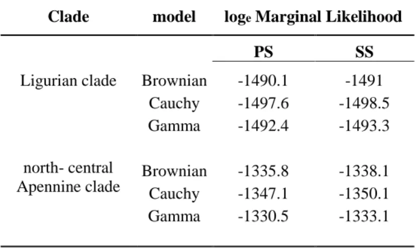
A run was generated for each spatial diffusion model (Brownian, Cauchy and Gamma), and the marginal likelihood (ML) of each model was estimated (MCMC length of 500 000, 100 path steps). Traces of the runs were inspected using Tracer, as above. The best model was evaluated using a Bayes factor, which was generated by confronting the path sampling and stepping-stone sampling estimates of the ML of each (Baele et al., 2012; Baele et al., 2013).
The best models for each lineage were visualized by projecting the maximum clade credibility (MCC) tree (selected by TreeAnnotator) and locations on a map using SPREAD 1.0.7 (Bielejec et al., 2011), and opening the “.kml” output file with Google Earth. The Time Slicer option in SPREAD was used to conduct an estimate of the 80% highest posterior density (HPD) of the spatial locations of the populations during their diffusion at four dates selected before the present [250 000 years ago (kya), 140 kya, 100 kya and the present] based on all of the trees obtained (the first 10% were removed as burn-in).
17
Descriptive statistics were obtained for the microsatellite dataset using FSTAT 2.9.3 (Goudet, 1995) in order to test for deviations from the expected Hardy-Weinberg and linkage equilibria, using the Bonferroni procedure to correct the significance level for multiple comparisons. GENETIX 4.05 (Belkhir et al., 1996) was used to obtain estimates of genetic diversity for each population, based on the mean observed and expected heterozygosity and the mean number of alleles.
Analysis of genetic structure
The population genetic structure across the study area was evaluated using the microsatellite and nuclear sequence datasets separately. We used a Bayesian clustering algorithm implemented in TESS 2.3.1 (Chen et al., 2007), with the spatial distribution of individuals as a prior, since it performs better than other Bayesian methods when the structure is not deep and/or there are not many loci (Chen et al., 2007; Francois & Durand, 2010). For the nuclear sequences dataset we compiled a genotype multilocus matrix using phased haplotypes as alleles. For both datasets, analyses were conducted by modelling admixture using a conditional autoregressive model (CAR). Preliminary analyses were conducted to assess model performance, with 20 000 runs (the first 5000 were discarded as burn-in) and 10 replicates for each K value (i.e. the number of clusters) between 2 and 10. The final analysis contained 100 replicates with K = 2–10, each with 50 000 runs (the first 20 000 were discarded as burn-in). The spatial interaction parameter was kept at the default value (0.6), and the option to update this parameter was activated. For both datasets, the model that best fitted the data was selected using the deviance information criterion (DIC). DIC values were averaged over the 100 replicates for each K value, and the most likely K value was selected as the one at which the average DIC reached a plateau. The estimated admixture proportions of the 10 runs with the lowest DIC values were averaged using CLUMPP 1.1.2 (Jakobsson & Rosemberg, 2007). The contribution of each obtained cluster in each population was represented in a pie chart. We obtained two separate graphs, one for the microsatellite dataset and one for the nuclear sequences dataset.
Species distribution model
In an attempt to locate hypothetical glacial and interglacial refugia for I. a. apuana, Species Distribution Models (SDMs) were used to forecast the bioclimatic suitability for
18
this species during the last glacial cycle. A maximum entropy modelling approach implemented in MAXENT 3.3.3k (Philips et al., 2006) was used to build a model of ecological niches of the species based on presence-only data. The model was built under current bioclimatic conditions and then projected onto reconstructions of past climatic conditions during the last interglacial phase (LIG, 120–140 kya) and last glacial maximum (LGM, 22 kya).
A total of 160 points of I. alpestris presence from all over its peninsular distribution (including the 15 sampling sites) were obtained from the literature and museum collections (Appendix I). The layers of bioclimatic data were downloaded from the WorldClim database (http:\\www.worldclim.org; Hijmans et al., 2005), with a 30-arc-second resolution for the current and the LIG and a 2.5-arc-minute resolution for the LGM; for the LGM we used predictions from both the Community Climate System Model (CCSM) and the Model for Interdisciplinary Research on Climate (MIROC). From 19 variables, we first excluded highly correlated variables (Pearson correlation coefficient r2>0,8) and then selected a subset of seven variables of major biological significance for I. alpestris, inferred from ecological studies (e.g. Fasola & Canova, 1992; Ambrogio & Gilli. 1998; Denoel et al., 2001; Kopecky et al, 2012) and SDM studies (Girardello et al., 2010) on this species. The variables were: the mean temperature of the wettest quarter (BIO8), the mean temperature of the driest quarter (BIO9), the mean temperature of the warmest quarter (BIO10), precipitation seasonality (BIO12), precipitation in the driest quarter (BIO17), precipitation in the warmest quarter (BIO18) and precipitation in the coldest quarter (BIO19). The layers were cropped to span from 4°1'30"E to 18°46'30"E and from 37°31'60"N to 48°40'30"N using DIVA-GIS 7.5 (Hijmans et al., 2001).
The model was built using MAXENT’s default parameters, with a convergence threshold of 10-5, 500 iterations and 10 000 random background points. Several tuning runs were conducted with different values (0.25 to 15) of the regularization multiplier parameter (Warren & Seifert, 2011; Radosavljevic & Anderson, 2014). To select the model that best fitted the data, we used the corrected Akaike Information Criterion (AICc) implemented in ENMTools (Warren et al., 2010). The definitive runs were performed in 10 replicates, with a sub-sample replicated run type and 25% of the data as a random test percentage. The mean value of the area under the curve (AUC) of a receiver-operating characteristic (ROC) plot was used to evaluate model performance (Araujo et al., 2005). The results of the two LGM projections were first evaluated individually and then averaged (Araujo et al., 2007).
20
2.3 RESULTS
For all individuals analysed we obtained a 399-bp fragment from CytB gene and an 878-bp fragment from ND2 gene (1277 878-bp in total). No indels, stop codons or non-sense codons were observed on either gene. In the combined mtDNA dataset, we found 13 haplotypes that were identified by 35 variable positions, 31 of which were parsimony informative. Mean haplotype diversity (h) and nucleotide diversity (π) values for this dataset were 0.803 (±0.019 SD) and 0.0077 (±0.0002 SD), respectively.
The nDNA dataset included a 328-bp fragment of β-FIB from 104 individuals, a 565-bp fragment of PDGFR from 111 individuals, and a 670-bp fragment of GH from 103 individuals. In the β-FIB alignments, we found six haplotypes that were identified by eight variable sites, seven of which were parsimony informative; h = 0.365 (±0.041 SD) and π = 0.0041 (±0.001 SD). In the PDGFR alignments, we found five haplotypes that were identified by four variable sites, four of which were parsimony informative; h = 0.413 (±0.038 SD) and π = 0.0018 (±0.0002 SD). In the GH alignments, we found eight haplotypes that were identified by 17 variable sites, 15 of which were parsimony informative; h = 0.376 (±0.039 SD) and π = 0.0017 (±0.0004 SD). No recombination events were indicated by the PHI tests conducted on the nuclear gene fragments (all P > 0.05). Using phased haplotypes as alleles, a multilocus genotype matrix was available from 121 individuals for the three nuclear loci, with 8% of the data missing. A full list of all the haplotypes found for each gene is presented in Table 3.
Phylogenetic data analysis
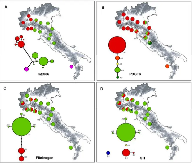
The phylogenetic network of the mtDNA haplotypes yielded by HaplotypeViewer is shown in Fig. 2. The log-likelihood score for the ML tree was -1963.08. We found three geographically distinct clades: a north-western Apennine clade (hereafter the Ligurian clade) that was poorly differentiated in the Piedmont population (sample 15), in all central and western Ligurian populations (samples 11–14) and at low frequency in an eastern Ligurian population (sample 10); a north-central Apennine clade that was more differentiated and found from eastern Ligurian to the central Apennine populations (samples 2–10); and the last clade consisted of a single haplotype, related to the north-central Apennine clade, and found exclusively in the Calabrian Apennine population
21
(sample 1). Interestingly, only within the geographically intermediate population of Mount Penna (sample 10) we found both the Ligurian and north-central Apennine clades. The statistical parsimony analysis showed the same clustering and topologies as the ML analysis, but two distinct networks were generated: one for the Ligurian clade and one for the north-central Apennine clade and the Calabrian clade (not shown). The mean Kimura 2-parameter sequence divergence value between the N-W and S-E clades was 0.012 (±0.003 SEM), between the S-E clade and the Calabrian haplotype was 0.007 (±0.002 SEM), and between the N-W and Calabrian clades was 0.015 (±0.003 SEM).
The phylogenetic networks among the haplotypes for each nuclear gene are shown in Fig. 2. In all cases, one single network connected all of the haplotypes, except for one haplotype in GH that did not connect with the main network. Despite all three genes showed low levels of variation, a geographical structure could be observed. In the β-FIB fragment, the most common haplotype was found spanning the whole range; it was the unique haplotype in central Italy, whereas it was found together with two different haplotypes in the Ligurian populations. A very similar pattern was found in the GH fragment; the differentiated haplotype was found at low frequencies, and exclusively in sample 9. In contrast, the opposite pattern was observed in the PDGFR fragment: the most common haplotype was the unique one found in the Ligurian populations, and its frequency gradually decreased towards the central Apennines, where three slightly differentiated haplotypes were found with growing frequency; in the Calabrian population, only one exclusive haplotype was found.
Divergence time estimation
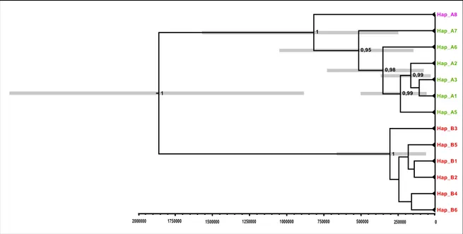
Both BEAST runs for the divergence time estimation converged to a stationary distribution, and had satisfactory ESS values that were largely above 200 for all the estimated parameters. After the two runs had been combined, the molecular substitution rate was 4.586 × 10⁻⁹ (95% HPD interval, 1.766 × 10⁻⁹, 8.08 × 10⁻⁹). The chronogram based on the MCC tree is shown in Fig. 3. The topology of the tree was in accord with the other analyses: a deep and ancient split was estimated between the N-W clade and the others (mean 1.86 million years ago (mya); 95% HPD interval, 0.89–2.86], whereas the separation between the Calabrian and north-central Apennine clade was more recent (mean 0.82 mya; 95% HPD interval, 0.25–1.57).
22
Bayesian spatial diffusion analysis
Spatial diffusion pattern analyses were performed on the Ligurian and north-central Apennine clades separately; the Calabrian clade was excluded from this analysis because it did not exhibit enough variation. All of the runs converged to a stationary distribution and showed satisfactory ESS values. The comparison of the different spatial diffusion models based on the ML estimates suggested that the Brownian model fitted the data better than Cauchy or Gamma models for Ligurian clade, whereas Gamma model fitted the data better than Brownian and Gamma for north-central Apennine clade. The loge ML values are
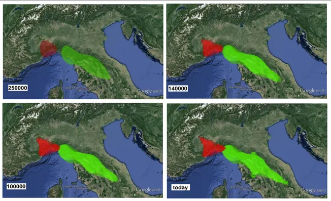
shown in Table 4. Therefore, since there were only slight differences in ML, the simplest Brownian model was selected to reconstruct phylogeographic diffusion patterns for both clades. The diffusion patterns during the time slices considered are shown in Fig. 4. This analysis localized the ancestral areas of the two lineages: one was in western Ligurian and the other in the Tuscan-Emilian Apennines. The first spread of both lineages occurred during the penultimate glacial phase, and before the beginning of the last interglacial phase, the two lineages had already realized a secondary contact in eastern Liguria. Any significant spatial expansion was not observed during the last interglacial, whereas a further spread was observed during the last glacial, during which I. alpestris probably colonized all of the areas that are currently occupied.
Microsatellite data analysis
A total of 185 individuals from 15 populations were genotyped at nine microsatellite loci. TaCa1 exhibited no variation across the samples and was excluded from further analyses. Ta2Caga3 was also removed, because it tested positive for null alleles in four populations. The final dataset consisted of a multilocus genotype for 185 individuals at seven microsatellite loci, with 2.8% of the data missing. We found significant deviation from the Hardy-Weinberg equilibrium in population 1 for TaCa1 and in population 13 for
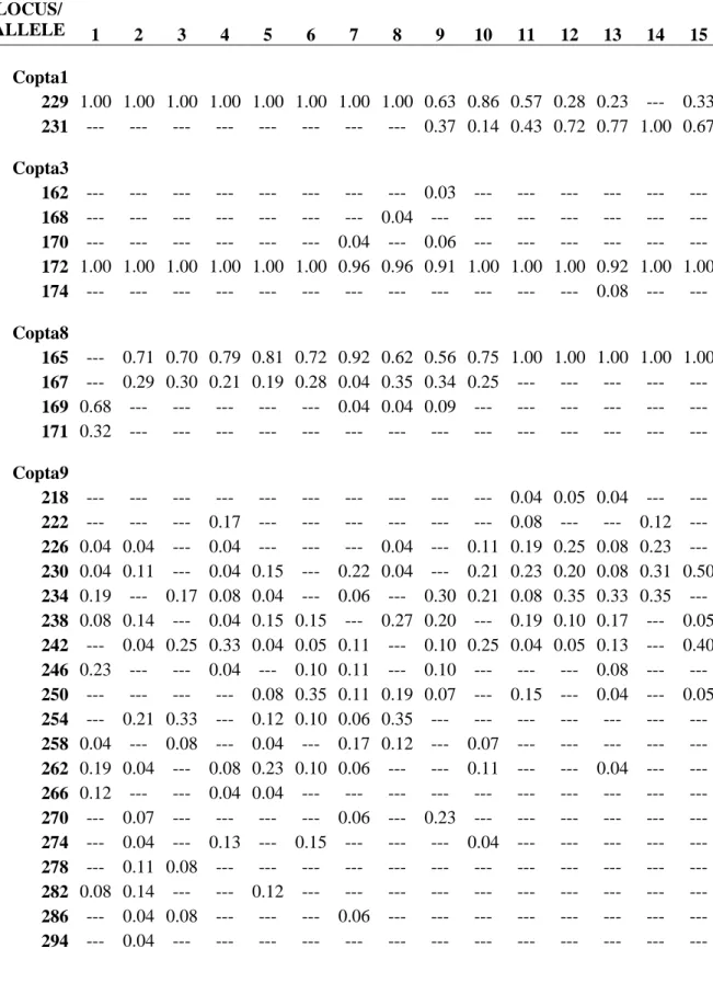
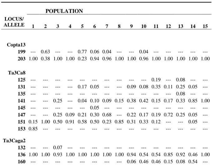
Copta9; no linkage disequilibrium was found. Across all populations, the number of alleles
at each locus ranged from 2 (Copta 13 and Copta 1) to 19 (Copta 9). The mean allelic richness and the mean expected heterozygosity for each population are presented in Table 1, and allelic frequencies for each locus and population are presented in Table 5.
23
Analysis of genetic structure
The analysis performed on the population genetic structure by TESS on the two datasets gave the same results and the same patterns of genetic variation across the populations. K = 3 was the best grouping option for the nuclear sequences dataset, because only a minor decrease in DIC values was observed at higher K values (Fig. 5a). The DIC curve in the microsatellite dataset analysis reached a plateau at K = 4 (Fig. 5b). However, an inspection of the plotted membership coefficients revealed that only three genetic clusters were present. It is not unusual for DIC to select models in which KMAX is greater than the
actual number of clusters (Durand et al, 2009; Temunovič et al., 2013). Bar plots showing the admixture proportion of each individual and pie charts showing the proportion of each group within each population are presented in Fig. 5. The spatial distribution of the genetic groups revealed a clear geographical structure that followed the one observed in the mtDNA data: one group consisted of the Ligurian populations, a second group included the north-central Apennine populations, and the third group contained only the Calabrian population. However, the level of population admixture was higher than that showed by the mtDNA; the geographically intermediate samples 9 and 10 were the most admixed populations, in which all of the individuals were admixed; admixture gradually decreased away from these populations. The nuclear sequences dataset had a higher proportion of admixture in the Ligurian populations, because all but one had other than 25% of other-group contributions, whereas only two populations in the north-central Apennine other-group were slightly admixed (samples 7 and 8).
Species distribution model
The model built with the value “1” as the regularization multiplier parameter was the one that best fitted our data (lowest AICc value). The average test AUC for the 10 replicate runs of the model was 0.966 (±0.010 SD), indicating a high and consistent performance (Araujo et al., 2005). Precipitation in the warmest quarter (BIO18) was the environmental variable with the highest percentage contribution and the highest gain when used in isolation; precipitation seasonality (BIO12) decreased the gain the most when omitted. MAXENT logistic output maps for the current model and for both past projections are shown in Fig. 6.
24
Under the present bioclimatic conditions, the SDM indicated that the Ligurian and Apuan Apennines are the most suitable areas, and the Tusco-Emilian Apennines are also suitable. These areas correspond to a great part of the I. a. apuana range. A slightly disjunct, suitable area was found in the central Apennines, from Gran Sasso and the Laga Mountains to the Majella Massif, where only one population has been recorded to date. The area where the relict Calabrian population survives was indicated as unsuitable by the current model. This pattern fits quite well with our current knowledge of the biology and distribution of I. alpestris on the Apennine Peninsula.
Both the CCSM and MIROC projections from the LGM predicted an expansion of suitable conditions for I. alpestris, but with a slightly different pattern between the two databases (data not shown). After the two projections were averaged, we observed three areas of major suitability: one in western Ligurian with the best values, a small, slightly separate one corresponding to the Apuan Apennines, and one that corresponded to the Latium and Abrutian Apennines. However, these areas were linked by large corridors of medium suitability in lowland areas of Latium and Tuscany. Projections from the LIG showed a marked reduction in suitable areas for this species. Good conditions were restricted to a narrow area in western Liguria and the northernmost Tusco-Emilian Apennines, and to small fragmented areas of the Latium and Abrutian Apennines. Overall, the SDM data indicated that climatic conditions for I. a. apuana were better during the LGM than at present, and even more so than during the LIG.
25
2.4 DISCUSSION
The genetic structure shown by I. alpestris on the Apennine Peninsula clearly reflects its ancient Pleistocene history, which was spent in at least three separate refugia where populations underwent strong genetic differentiation. This pattern is in agreement with the precedent evidences of multiple genetic lineages within the “apuana clade”, as suggested by the species phylogenies of Sotiropoulus et al., (2007) and Recuero et al., (2014). Nevertheless, our denser sampling scheme, coupled with the use of more markers, has clarified the geographical structure and the amount of such genetic variation.
Both the mitochondrial and nuclear markers identified three main genetic lineages that were strongly differentiated, one restricted to the southernmost populations in Calabria, one ranging from the northern to the central Apennines, and one ranging from the western to the eastern Ligurian Apennines. The Calabrian populations are more than 500 km from the nearest population in the central Apennines, and show genetic divergence of a mid-Pleistocene origin, confirming that it is a biogeographical relict. The low level of genetic diversity found might be attributable to significant inbreeding, since the population size was estimated to be only around 300 individuals (Dubois & Ohler, 2009). However, despite a greater divergence, the other two lineages have actually a contiguous distribution and co-occur in a contact zone in the eastern Ligurian Apennines, where the populations are strongly admixed. Interestingly, the contact zone is wider for nuclear genes than mitochondrial genes, because only one population shares the mitochondrial haplotypes of both lineages. This type of mito-nuclear discordance can be explained by male-biased dispersal (Toews & Brelsford, 2012), which might result in faster movement of nuclear genes (biparental) than mitochondrial genes (only matrilineal). Male-biased dispersal has been reported in juvenile I. alpestris (Joly & Grolet, 1996), and was previously invoked to explain mito-nuclear discordance in this species (Recuero et al., 2014). In addition, male-biased dispersal could have been increased by the high prevalence of paedomorphic females in the Apennine populations, because paedomorphic individuals do not disperse (Denoel et al, 2001).
The contact zone falls in an area of great biogeographical interest, since other taxa have shown traces of secondary contacts among closely related lineages, particularly among mountain species (e.g. Porter et al, 1997; Cimmaruta et al, 2015). Moreover this area marks the range boundary of several taxa, including amphibians (Hyla meridionalis,
26 Pelodytes punctatus and Rana italica), suggesting that it might exhibit, or have exhibited,
peculiar climatic or geographical characteristics. Nevertheless, since strong geographical discontinuities in this area were hitherto not reported as a possible causal factor, the hypothesis that peculiar climatic conditions could have affected the evolutionary histories of these species remains the most probable explanation. The Apennines are particularly close to the sea in this area, a situation that strongly affects the climate (Rapetti & Vittorini, 2013) and might have affected the climate during past glacial cycles. In addition, the Ligurian Apennines was already indicated as a crossway during recolonization pathway of several taxa, which have differentiated inside and outside the peninsula in Western Europe, including the Alps (Taberlet, 1998; Hewitt, 1999). All of these factors make this area an interesting hotspot of biodiversity, as well as a hotspot of evolutionary and biogeographical processes, increasing the interest on dynamics involved in the evolutionary history of inhabiting species.
Evolutionary history of I. alpestris on the Apennine Peninsula
The strong genetic differentiation found among the Apennine lineages of I. alpestris, and even more so among these lineages and other European ones, suggests an evolutionary history of ancient origin. The estimated time to the most recent common ancestor (TMRCA) among Apennine and other European lineages is 9.2 ± 2.1 mya (Recuero et al. 2014), suggesting that I. alpestris may have colonized the Apennine Peninsula during the Late Miocene. This period coincided with the establishment of the first connection between the Apennine Peninsula and Europe (Popov et al., 2004), which resulted in the immigration of several faunal elements from Europe (Rook et al., 2006). However, the biogeographical connection was repeatedly interrupted from the Late Miocene until the Middle Pliocene by the long submersion of the Northern Apennines, which was caused by eustatic variations in sea level (Ghibaudo et al., 1985; Yilmaz, et al., 1996; Rook et al., 2006). These long interruptions probably caused the isolation and differentiation of peninsular populations of I. alpestris from European populations, as has been observed for several other taxa that exhibit a coeval split (Cimmaruta et al., 2015).
Thereafter, the evolutionary history of I. alpestris on the Apennine Peninsula seems to have been strongly linked to the large climatic revolutions of the Pleistocene, since splits between the main genetic lineages are estimated to have occurred in the Early Pleistocene and in the beginning of the Middle Pleistocene. The split between the Ligurian and central
27
Apennine lineages was estimated to have occurred during the Early Pleistocene (1.86 mya ± 1.0), which coincided with a general cooling of the Northern Hemisphere that was caused by the effects of the first major glacial cycles (Kahlke et al., 2011). Because of this cooling, frigophilous species such as I. alpestris might have initially benefited from the spread of suitable habitats at lower altitudes and latitudes, and might have expanded their ranges along the peninsula. A general spread of other cold-adapted taxa during the Early Pleistocene has been reported by Bertini (2003, 2010), Masini & Sala, (2007) and Kahlke
et al. (2011). Nevertheless, the effects of climatic instability, presumably the effects of the warm interglacials, might have fragmented the distributions of these species after the early expansion, trapping populations within small areas. I. alpestris is a short range disperser (Joly & Miaud, 1989), and populations might not have had sufficient time to return in contact during favourable phases, since cold phases in the Early Pleistocene were shorter than the last glacial phases (Head & Gibbard, 2005). In addition, population isolation may have been increased by paedomorphism, which probably evolved as an adaptation to Quaternary climatic instability by not encouraging dispersal from relatively stable habitats and refugia. Moreover, other species inhabiting mountain habitats have exhibited vicariance in the Ligurian Apennines from the Early Pleistocene (eg. Hydromantes, Cimmaruta et al., 2015), suggesting that they had common biogeographical and evolutionary pathways.
The TMRCA of the Calabrian and central Apennine lineages was estimated to be around 800 kya, which coincided with the Mid-Pleistocene revolution. This period was characterized by an increase in the amplitude and length of glacial cycles (from 40 to 100 kya) that had major biogeographical effects (Head & Gibbard, 2005; Hewitt, 2011a). The Italian Peninsula saw large changes in community assemblages (Capraro et al., 2005; Palombo et al, 2005), and several species’ ranges underwent severe fragmentation that was followed by genetic differentiation (Canestrelli et al., 2012b; Maura et al, 2014). However, two particularly humid glacial cycles [corresponding to Marine Isotope Stage (MIS) 20 and MIS 18, which were 750–850 kya] caused the expansion of alpine forests in Calabria (Capraro et al., 2005), and might have favoured a southward expansion of I. alpestris that was closely linked with mountain forest habitats. Such a great expansion may never have been repeated, because we did not find any traces of successive contacts between the two lineages, which have accumulated large genetic differences.
In contrast, the secondary contact between the Ligurian and central Apennine lineages was estimated to be during the Late Pleistocene. Our spatiotemporal
28
phylogeographical reconstruction of the last phases of the Pleistocene showed that most of the expansion from the Ligurian and central Apennine refugia had already occurred at the end of the penultimate glacial period, which supports the hypothesis that I. alpestris populations underwent major expansions during the cold, glacial phases. Nevertheless, the penultimate glacial (MIS 6) was particularly cold and humid, and was interspersed by several interstadials with intermediate climate (Roucoux et al, 2011; Wainer et al., 2012; Litt et al., 2014). Such an unusual condition for a glacial stage favoured the expansion of montane tree forests in southern Europe (Roucoux et al, 2011), and may have favoured a greater expansion of I. alpestris from its refugia. However, at the beginning of the last interglacial, the two lineages had already established a secondary contact in eastern Liguria. The contact probably persisted during the last interglacial, because the SDM projection indicated that the contact zone was suitable for this species during the interglacial, suggesting that it was an interglacial refugium. Nevertheless, the SDM supported the hypothesis that there was a reduction in suitable bioclimatic conditions for this species during the interglacial and it expanded during glacial periods, despite the fact that the suitable area was more fragmented during the LGM. Despite the fragmentation and the fact that some putative, suitable areas were covered by ice, e.g. the Apuan and central Apennines (Ehlers & Gibbard, 2004), the Bayesian phylogeographical reconstruction indicated a further expansion of I. alpestris during the last glacial phase.
The genetic diversity distribution analysis of the I. alpestris populations revealed some interesting patterns. Haplotype diversity within each group, and within each population, was low compared to that of other peninsular amphibians (Lissotriton italicus, Canestrelli et al, 2012a; Triturus carnifex, Canestrelli et al, 2012b; L. vulgaris, Maura et
al, 2014), but was similar to that of other cold-adapted amphibians, such as Rana temporaria (Stefani et al., 2012). The population genetic diversity as revealed by the
microsatellite markers was low compared to that of other European populations of the same species (Pabijan & Babik, 2006; Prunier et al., 2014; Emaresi et al, 2011). These low levels of genetic diversity could have been caused by repeated bottlenecks of the Apennine populations during the Pleistocene, as well as the fragmentation and isolation of the peninsular populations. The lowest values of genetic diversity were exhibited by the southernmost and northernmost populations (samples 1 and 15). Nevertheless genetic diversity increased towards the core of the species’s range. We found the highest levels of genetic diversity within the populations inside the contact zone, where all individuals were highly admixed with genetic components from the different lineages. Other peninsular taxa
29
have shown similar patterns, with the highest genetic diversity within the contact zones of different intraspecific lineages, rather than inside the refugia of such lineages (Canestrelli
et al., 2008, 2010). This does not support the hypothesis that high levels of biodiversity
within southern European peninsulas were caused by the relative stability of refugia, but highlights the importance of sub-refugia in shaping genetic variation and of melting-pot areas in reshuffling such variation and increasing biodiversity.
30
2.5 TABLES AND FIGURES
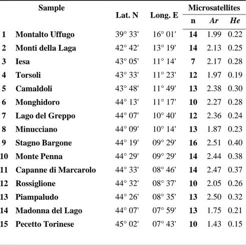
Table 1 Geographic location, and estimates of genetic variability at microsatellite loci for
each of the 15 sampling sites of Ichthyosaura alpestris. n, sample size; Ar, Allelic richness; He, expected heterozygosity.
Sample
Lat. N Long. E Microsatellites n Ar He
1 Montalto Uffugo 39° 33' 16° 01' 14 1.99 0.22
2 Monti della Laga 42° 42' 13° 19' 14 2.13 0.25
3 Iesa 43° 05' 11° 14' 7 2.17 0.28
4 Torsoli 43° 33' 11° 23' 12 1.97 0.19
5 Camaldoli 43° 48' 11° 49' 13 2.38 0.30
6 Monghidoro 44° 13' 11° 17' 10 2.27 0.28
7 Lago del Greppo 44° 07' 10° 40' 12 2.36 0.24
8 Minucciano 44° 09' 10° 14' 13 1.87 0.23 9 Stagno Bargone 44° 19' 09° 29' 16 2.51 0.40 10 Monte Penna 44° 29' 09° 29' 14 2.44 0.38 11 Capanne di Marcarolo 44° 33' 08° 46' 14 2.47 0.37 12 Rossiglione 44° 32' 08° 37' 10 2.05 0.26 13 Piampaludo 44° 26' 08° 35' 13 2.50 0.32
14 Madonna del Lago 44° 07' 07° 59' 13 1.75 0.21
15 Pecetto Torinese 45° 02' 07° 43' 10 1.43 0.15
31
Table 2 PCR primers and annealing temperatures used to amplify the two mitochondrial
and three nuclear DNA fragments used in this study. References: (1) Canestrelli et al., 2006a; (2) Nadachowska & Babik, 2009; (3) Sequeira et al., 2006.
Marker Primers (5' -> 3') annealing
T (°C) References
CytB CytBtrit-F F: ACGCAAYATRCACATCAACGG
53
1
CytBtrit-R R: GGAGTGACTATAGARTTTGCTGGG 1
NADH2 L3780mod2 F: GGAGAAACCCCTTCTTTTGC
59
This study
H5018mod1 R: TGAAGGCCTTTGGTCTTGTTAT This study
GH GH-f F: TCTCATCAAGGTGAGTTTGAACA 58 2 GH-r R: CCTTCTTGTGTCAGAGGTGCTAT 2 PDGF-R Pdgfr-F F: TGCAGCTGCCATATGACTCTA 60 2 Pdgfr-R R: TACGCTGTTCCTTCAACCACT 2
β-FIB FibX7 F: GGAGANAACAGNACNATGACAATNCAC
50 3 FibX8 R: ATCTNCCATTAGGNTTGGCTGCATGGC 3 BFXF F: CAGYACTTTYGAYAGAGACAAYGATGG 59 3 BFXR R: TTGTACCACCAKCCACCRTCTTC 3
32
Table 3 List of haplotypes found for each studied gene in each studied population. n,
sample size; among brackets the number of haplotypes found.
Sample
Haplotypes
n mtDNA n β - Fibrinogen n PDGFR n GH
1 11 AVIII 6 AI(6), AII(6) 9 AII 9 AI(18)
2 10 AI 7 AI 7 AI(1), AIV(4),
AV(9)
7 AI(14) 3 4 AI(3), AIII(1) 4 AI 4 AI(6), AIV(2) 4 AI(8)
4 9 AI(9) 9 AI 8 AI(9), AIV(7) 7 AI(12), AII(2)
5 11 AI(4), AII(7) 6 AI 6 AI 6 AI(12)
6 7 AI 8 AI 5 AI(5), AIV(5) 7 AI(10), AII(3),
AVI(1)
7 9 AI(8), AV(1) 11 AI 10 AI(15), AIII(1),
AIV(4)
10 AI(19), AII(1)
8 10 AI 8 AI 8 AI(11), AIV(5) 8 AI(16)
9 14 AVI(13),
AVII(1)
11 AI(13), AIV(2),
B1(5), BII(2)
14 AI 8 AI(12), C(4)
10 14 AVI(12), BII(2) 8 AI(13), AIII(1),
BII(2)
9 AI 7 AI(9), BI(5)
11 9 BI(8), BVI(1) 5 AI(4), BI(4), BII(2) 6 AI 5 AI(6), BI(4) 12 9 BI 5 AI(4), BI(4), BII(2) 5 AI 4 AI(5), AIII(2),
BI(1)
13 12 BI(3), BIV(2),
BV(1), BIII(6)
6 AI(6), BI(6) 8 AI 7 AI(11), BI(3)
14 10 BII 5 BII(8), AI(2) 5 AI 6 AI(3), AV(1),
BI(7), BII(1)
15 10 BI 5 AI 7 AI 8 AI(5), BI(10),