Advanced Techniques for Image Analysis and Enhancement

D

R

I

– XXIII ciclo

Tesi di Dottorato

Advanced Techniques for Image

Analysis and Enhancement

Applied Image Processing Algorithms for Embedded Devices

Giuseppe MESSINA

Tutor Coordinatore

I would like to take this opportunity to thank all my colleagues at the Advanced System Technology, Catania Lab (STMicroelectronics) and the whole Image Processing Lab (Catania University) in particu-lar prof. Battiato for his patience. A special thanks also to Valeria and Mirko for our big achievements, and to Giovanni Maria and Daniele for the excellent job. Finally I would like to acknowledge Tony and Rosetta for their valuable companionship on the long way to our final Ph.D. target. After three years on my shoulders I will certainly miss them.

Preface

1

I

Image Processing for Embedded Devices

11

1 Color Interpolation and False Color Removal 13

1.1 Color Interpolation Techniques . . . 19

1.1.1 Spatial-Domain Approaches . . . 19

1.1.2 Frequency-domain Approaches . . . 37

1.2 Techniques for Aliasing Correction . . . 50

1.2.1 False Colors Cancelling . . . 53

1.2.2 Zipper Cancelling . . . 63

2 An Adaptive Color Interpolation Technique 67 2.1 Color Interpolation . . . 67

2.1.1 Direction Estimation Block . . . 68

2.1.2 Neighbor Analysis . . . 75

2.1.3 Interpolation . . . 81

2.2 False Colors Removal . . . 85

2.3 Experimental Results . . . 90

II

Image Analysis and Enhancement

105

3 Red Eyes Removal 107

3.1 Introduction . . . 107

3.2 Prior Art . . . 111

3.2.1 Eye Detection . . . 111

3.2.2 Red Eye Correction . . . 123

3.2.3 Correction Side Effects . . . 128

3.2.4 Quality Criteria . . . 131

3.3 A New Red-Eyes Detection and Correction Technique . . . 134

3.3.1 Red Patch Extraction . . . 134

3.3.2 Red Patch Classification . . . 139

3.3.3 Boosting for binary classification exploiting gray codes . 142 3.3.4 Red-Eyes Correction . . . 144

3.3.5 Experimental Settings and Results . . . 147

3.4 Conclusion and Future Works . . . 153

4 Exposure Correction Feature Dependent 155 4.1 Introduction . . . 155

4.2 Exposure Metering Techniques . . . 157

4.2.1 Classical Approaches . . . 159

4.2.2 Advanced Approaches . . . 162

4.2.3 Exposure Control-System . . . 164

4.3.1 Feature Extraction . . . 167

4.3.2 Exposure Correction . . . 174

4.3.3 Results . . . 175

4.4 Conclusion . . . 177

III

Forensics Image Processing

181

5.2 DCT Quantization . . . 186

5.3 State of the Art Analysis . . . 187

5.4 Dataset and Discussion . . . 192

5.5 Acknowledgments . . . 197 5.6 Conclusions . . . 197 6 Chain of Evidence 199 6.1 Introduction . . . 199 6.2 Image Analysis . . . 201 6.2.1 Features Extraction . . . 201 6.2.2 Features Analysis . . . 203 6.2.3 Script Generation . . . 204 6.3 Experiments . . . 205 6.4 Conclusion . . . 207

Preface

The research activities, described in this thesis, have been mainly focused on images analysis and quality enhancement. Specifically the research regards the study and development of algorithms for color interpolation, contrast enhance-ment and red-eye removal, which have been exclusively oriented to mobile de-vices. Furthermore an images analysis for forgeries identification and image enhancement, usually directed by investigators (Forensic Image Processing) has been conducted.

The thesis is organized in three main parts: Image Processing for Embedded Devices; Image Analysis and Enhancement; Forensics Image Processing.

Image Processing for Embedded Devices

Imaging consumer, prosumer and professional devices, such as digital still and video cameras, mobile phones, personal digital assistants, visual sensors for surveillance and automotive applications, usually capture the scene content by means of a single sensor (CCD or CMOS), covering its surface with a Color Fil-ter Array (CFA), thus significantly reducing costs, sizes and registration errors. The most common arrangement of spectrally selective filters is known as Bayer pattern [25]. This simple CFA, taking into account human visual system charac-teristics , consists of a simple RGB lattices and contains twice as many green as red or blue sensors (human eyes are more sensitive to green with respect to the other primary colors)[BCGM10]. Some spatially undersampled color channels are then provided by the sensor and the full color information is reconstructed by color interpolation algorithms (demosaicing) [GMTB08]. Demosaicing is a very critical task. A lot of annoying artifacts that heavily degrade picture quality

can be generated in this step: zipper effect, false color, etc. False colors are ev-ident color errors which arise near the object boundaries, whereas zipper effect artifacts manifest as “on-off” patterns and are caused by an erroneous interpola-tion across edges. The green channel is less affected by aliasing than the red and blue channels, because it is sampled at a higher rate. Simple intra-channel in-terpolation algorithms (e.g., bilinear, bicubic) cannot be then applied and more advanced solutions (inter-channel), both spatial and frequency domain based, have been developed [GMT10a]. In embedded devices the complexity of these algorithms must be pretty low. Demosaicing approaches are not always able to completely eliminate false colors and zipper effects, thus imaging pipelines of-ten include a post-processing module, with the aim of removing residual artifacts [TGM09].

It is worthwhile to understand that picture quality is strictly related not only to the number of pixels composing the sensor, but also to the quality of the demosaicing algorithm within the Image Generation Pipeline (IGP). The IGP usually consists of a preprocessing block (auto-focus, auto-exposure, etc.), a white balancing, a noise reduction, a color interpolation, a color matrixing step (that corrects the colors depending on the sensor architecture), and postprocessing blocks (sharp-ening, stabilization, compression, red-eyes removal, etc.) [BBMP10,BCM10]. Color interpolation techniques should be implemented by considering the arti-facts introduced by the sensor and the interactions with the other modules com-posing the image processing pipeline, as it has been well analyzed in [5]. This means that demosaicing approaches have to guarantee the rendering of high quality pictures avoiding typical artifacts, which could be emphasized by the sharpening module, thus drastically deteriorating the final image quality. In the meantime, demosaicing should avoid introducing false edge structures due to

residual noise (not completely removed by the noise reduction block) or green imbalance effects. Green imbalance is a mismatch arising in some sensors be-cause the photosensitive elements that capture G intensity values at GRlocations

can have a different response than the photosensitive elements that capture G intensity values at and GB locations. This effect is mainly due to crosstalk [73].

In order to broaden the know-how and to allow an efficient study of the state of the art in the color interpolation field, an extensive patent research has been performed, since this problem dealt with industrial processes [BGMT08]. In Chapter 1 we describe the state of the art of demosaicing techniques. A com-plete excursus on color interpolation techniques is described, from spatial to frequency domain approaches, also in terms of color artifacts removal. Thus in Chapter 2 a new color interpolation technique, developed for embedded de-vices, is described. The method has been compared with other state of the art approaches and has shown good performances both in term of color reconstruc-tion and artifact reducreconstruc-tion. Furthermore it has been established that the method is also able to drastically reduce residual noise, preserving details [GMT10].

Image Analysis and Enhancement

Red-eye artifact is caused by the flash light reflected off a person’s retina. This effect often occurs when the flash light is very close to the camera lens, as in most compact imaging devices. To reduce these artifacts, most cameras have a red-eye flash mode which fires a series of pre-flashes prior to picture capturing. Rapid pre-flashes cause pupil contraction thus minimizing the area of reflection; it does not completely eliminate the red-eye effect, though reduces it. The major disadvantage of the pre-flash approach is power consumption (e.g., flash is the

most power-consuming device of the camera). Besides, repeated flashes usually cause uncomfortable feeling.

Alternatively, red-eyes can be detected after photo acquisition. Some photo-editing software make use of red-eye removal tools which require considerable user interaction. To overcome this problem, different techniques have been pro-posed in literature (see [56, 106] for recent reviews in the field). Due to the growing interest of industry, many automatic algorithms, embedded on commer-cial software, have been patented in the last decade [57]. The huge variety of approaches has permitted to explore different aspects of red-eyes identification and correction [BFGMR10,BFMGR10b]. The big challenge now is to obtain the best results with the minor number of visual errors.

To this end, several low-level feature eyes classification techniques have been analyzed [BGMM09,GGMT10]. This has allowed us to identify a methodology that has improved the performance of the techniques previously developed at the state of the art. In Chapter 3 we provide an overview of well-known automatic red eye detection and correction techniques, pointing out working principles, strengths and weaknesses of the various solutions [MM10]. Finally we describe our advanced red-eyes removal pipeline (see section 3.3). After an image filter-ing pipeline devoted to select only the potential regions in which red-eye arti-facts are likely to be, a cluster-based boosting on gray codes based features is employed for classification purpose. Red-eyes are then corrected through de-saturation and brightness reduction. Experiments on a representative dataset confirm the real effectiveness of the proposed strategy which also allows to properly managing the multi-modally nature of the input space. The obtained results have pointed out a good trade-off between overall hit-rate and false pos-itives. Moreover, the proposed approach has shown good performance in terms

of quality measure [BFGMR10a]. This activity has also produced the filling of a patent application to the Italian patent office [MGF09] and its extension to the U.S. patent office (which is at a preliminary stage).

Finally we have faced the exposure correction of wrongly acquired images. The problem of the proper exposure settings for image acquisition is of course strictly related with the dynamic range of the real scene [BMC08]. In many cases some useful insights can be achieved by implementing ad-hoc metering strategies. Al-ternatively, it is possible to apply some tone correction methods that enhance the overall contrast of the most salient regions of the picture. The limited dynamic range of the imaging sensors doesn’t allow to recover the dynamic of the real world. In Chapter 4 we present a brief review of automatic digital exposure cor-rection methods trying to report the specific peculiarities of each solution. Start-ing from exposure meterStart-ing techniques, which are used to establish the correct exposition settings, we describe automatic methods to extract relevant features and perform corrections [CM10].

Forensics Image Processing

The analysis and improvement of image quality, for forensic use, are the sub-ject of recent studies and have had a major boost with the advent of the digital imaging [12]. In this context it was agreed to deal with two different aspects of the image processing for forensics use: tampering identification into digital im-ages (through the analysis of available data) and quality improvement of digital evidence for investigations purpose.

Nowadays the ubiquity of video surveillance systems and camera phones have made available a huge amount of digital evidences to the investigators [BFMP10, BM10a]. Unfortunately one of the main problem is the malleability of digital

images for manipulation. Hence the detection of tampering into digital images is a research topic of particular interest, both in academia contents, as evidenced by the recent literature, and in forensics field, as there are several requirements to validate the reliability of digital evidence in legal processes [BMR09].

One of the existing approaches considers the possibility of exploiting the statis-tical distribution of DCT coefficients of JPEG images in order to reveal the ir-regularities due to the presence of a signal superimposed onto the original (e.g., due to copy and paste). As recently demonstrated [45–48], the relationship be-tween the quantization tables used to compress the signal, before and after the forgery, highlights anomalies in the histograms of DCT coefficients, especially for certain frequencies.

Starting from an initial study of the prior art some preliminary results of the detection of forgery (i.e., detection of tampering of the image) have been pre-sented to the anti-pedophilia group (Crime Against Children) at Interpol in Lyon (France). This presentation formed the basis for a possible collaboration with international intelligence agencies and allowed the identification of the issues of existing approaches. The research was then directed to a detailed analysis of the performance of existing approaches to assess their effectiveness and weaknesses, and then outlined the basis for the implementation of an approach robust enough to deal with quality tests disappointed by the existing methods. The first results obtained from the analysis of robustness of some algorithms were then presented at an international conference [BM09]. These studies, described in Chapter 5, have highlighted the gaps in the known techniques and also has emphasized the need to create a database of forged images [BMT10], which could be candidate as reference point for the scientific community [81].

The second research field, described in Chapter 6, involves the quality improve-ment of data for investigative use. The quality of images obtained from digital cameras and camcorders today is greatly improved since the first models of the eighties. Unfortunately it is still not unusual, in the forensic field, to get into images wrongly exposed, noisy and/or corrupted by motion blur. This is often due to the presence of old devices or to an illumination of the scene that does not allow a correct acquisition (for example in night shots). Extrapolating some details, normally invisible to human eye, by improving the quality of the image, is of crucial aspect to facilitate investigations [BMS10]. The current rules, for the production of forensic digital material, require to fully document the steps of images processing, in order to allow the exact replication of the enhance-ment [1, 3]. The automation of image enhanceenhance-ment techniques are therefore required and must be thoroughly documented. This chapter describes a tool for the automation of image enhancement technique, that allows both the automatic image correction and the generation of a script able to repeat the chain of en-hancement steps. This work has been developed through a request received from the RIS (Scientific Investigations Department) of Messina (Italy), which has ex-pressed a strong interest into this research area.

Personal Bibliography

[GMTB08] M.I. Guarnera, G. Messina, V. Tomaselli, and A. Bruna. Directionally filter based demosaicing with integrated antialiasing. In Proc. of the In-ternational Conference in Consumer Electronics, Las Vegas (NE), Jan-uary 2008. ICCE 2008.

[BGMT08] S. Battiato, M.I. Guarnera, G. Messina, and V. Tomaselli. Recent patents on color demosaicing,. Recent Patents on Computer Science, Bentham Science Publishers Ltd, 1(2), 2008.

[BMC08] S. Battiato, G. Messina, and A. Castorina. Single-Sensor Imaging: Methods and Applications for Digital Cameras, chapter 12.Exposure

Correction for Imaging Devices: an Overview, pages 323 – 349. CRC Press, 2008. ISBN: 978-1420054521.

[TGM09] V. Tomaselli, M.I. Guarnera, and G. Messina. False-color removal on the ycc color space. In Proc. of the IS&T/SPIE Electronic Imaging 2009, San Jose (CA), January 2009. SPIE 2009.

[BGMM09] S. Battiato, M. Guarnera, T. Meccio, and G. Messina. Red eye detection through bag-of-keypoints classification. In Berlin Heidelberg 2009, ed-itor, LNCS 5646, pages 180 – 187, Salerno,Italy, September 2009. 15th International Conference on Image Analysis and Processing, Springer-Verlag.

[BM09] S. Battiato and G. Messina. Digital forgery estimation into dct domain - a critical analysis. In ACM Multimedia 2009 Workshop Multimedia in Forensics, Beijing, China, October 2009. ACM.

[BMR09] S. Battiato, G. Messina, and R. Rizzo. IISFA Memberbook 2009, Dig-ital Forensics, Condivisione della conoscenza tra i membri dell’IISFA ITALIAN CHAPTER, chapter 1. Image Forenscis: Contraffazione Digi-tale e Identificazione della Camera di Acquisizione: Status e Prospettive, pages 1–48. International Information Systems Forensics Association, Dicembre 2009.

[MGF09] G. Messina, M. Guarnera, and G. M. Farinella. Method and Appa-ratus for Filtering Red and/or Golden Eye Artifacts in Digital Images Italian Patent Pending, 18 December 2009, Application number IT-RM09A000669.

[GGMT10] M. Guarnera, I. Guarneri, G. Messina, and V. Tomaselli. A signature analysis-based method for elliptical shape detection. In Proc. of the IS’T/SPIE Electronic Imaging 2009, San Jose (CA), January 2010. SPIE 2010.

[BMS10] S. Battiato, G. Messina, and D. Strano. Chain of evidence generation for contrast enhancement in digital image forensics. In Proc. of the IS’T/SPIE Electronic Imaging 2009, San Jose (CA), January 2010. SPIE 2010.

[GMT10] M. Guarnera, G. Messina, and V. Tomaselli. Adaptive color demosaicing and false color removal. Journal of Electronic Imaging, Special Issue on Digital Photography, SPIE and IS&T, 19(2):021105–1–16, Apr-Jun 2010.

[BMT10] S. Battiato, G. Messina, and L. Truppia. An improved benchmarking dataset for forgery detection strategies. In Minisymposium on Image and Video Forensics, Cagliari (Italy), June 2010. SIMAI.

[BFGMR10] S.Battiato, G.M. Farinella, M. Guarnera, G. Messina, and D. Rav`ı. Boosting gray codes for red eyes removal. In International Conference on Pattern Recognition ICPR 2010, pages 1–4, Instanbul (TK), August 2010.

[BFGMR10a] S.Battiato, G.M. Farinella, M. Guarnera, G. Messina, and D. Rav`ı. Red-eyes removal through cluster based linear discriminant analysis. In IEEE ICIP 2010 - International Conference on Image Processing, pages 1–4, Hong Kong, September 2010.

[BFGMR10b] S. Battiato, G.M. Farinella, M. Guarnera, G. Messina, and D. Rav`ı. Red-eyes removal through cluster based boosting on gray codes. EURASIP Journal on Image and Video Processing, Special Issue on Emerging Methods for Color Image and Video Quality Enhancement, pages 1– 19,ISSN: 1687-5176, 2010.

[BBMP10] S. Battiato, A. Bruna, G. Messina, and G. Puglisi. Image Process-ing for Embedded Devices - From CFA data to image/video codProcess-ing , eBook, Bentham Science Publishers Ltd., eISBN: 978-1608051700, vol.1, November 2010.

[BCGM10] A. R. Bruna, A. Capra, M. Guarnera, and G. Messina. Image Processing for Embedded Devices - From CFA data to image/video coding, vol-ume 1, chapter 2. Notions about Optics and Sensors. S. Battiato and A. Bruna and G. Messina and G. Puglisi, eBook, Bentham Science Pub-lishers Ltd., eISBN: 978-1608051700, vol.1, November 2010.

[CM10] A. Castorina and G. Messina. Image Processing for Embedded Devices - From CFA data to image/video coding, volume 1, chapter 3. Exposure Correction. S. Battiato and A. Bruna and G. Messina and G. Puglisi, eBook, Bentham Science Publishers Ltd., eISBN: 978-1608051700, vol.1, November 2010.

[GMT10a] M. Guarnera, G. Messina, and V. Tomaselli. Image Processing for Em-bedded Devices - From CFA data to image/video coding, volume 1, chap-ter 7. Demosaicing and Aliasing Correction. S. Battiato and A. Bruna and G. Messina and G. Puglisi, eBook, Bentham Science Publishers Ltd., eISBN: 978-1608051700, vol.1, November 2010.

[MM10] T. Meccio and G. Messina. Image Processing for Embedded Devices -From CFA data to image/video coding, volume 1, chapter 8. Red Eyes Removal. S. Battiato and A. Bruna and G. Messina and G. Puglisi, eBook, Bentham Science Publishers Ltd., eISBN: 978-1608051700, vol.1, November 2010.

[BCM10] S. Battiato, A. Castorina, and G. Messina. Image Processing for Em-bedded Devices - From CFA data to image/video coding, volume 1, chapter 13. Beyond Embedded Devices. S. Battiato and A. Bruna and G. Messina and G. Puglisi, eBook, Bentham Science Publishers Ltd., eISBN: 978-1608051700, vol.1, November 2010.

[BFMP10] S. Battiato, G.M. Farinella, G. Messina, and G. Puglisi. IISFA Member-book 2010, Digital Forensics, Condivisione della conoscenza tra i mem-bri dell’IISFA ITALIAN CHAPTER, chapter 11. Digital Video Forensics: Status e Prospettive, pages 271-296. International Information Systems Forensics Association, December 2010. in press.

[BM10a] S. Battiato and G. Messina Video digitali in ambito forense. In Ciberspazio e Diritto, vol. IV, 2010, in press.

Image Processing for Embedded

Devices

1. Color Interpolation and False

Color Removal

The simplest demosaicing (or color interpolation) method is the bilinear inter-polation, a proper average on each pixel depending on its position in the Bayer Pattern. For a pixel, we consider its eight direct neighbors and then we determine the two missing colors of this pixel by averaging the colors of the neighboring ones. We actually have 4 different cases of averaging which correspond to the red pixel, the blue pixel, the green pixel on a red row and the green pixel on the blue row. On each of them, the averaging will be slightly different. Assuming the notation used in Fig.(1.1) and considering, as example, the pixels R33, B44,

G43 and G34, the bilinear interpolation proceeds as follows:

G₁₂ R₁₃ G₁ R₁₁ G21 B22 G23 B2 GG₁₂₃₂ RR₁₃₃₃ GG₁₄₃ R₃₁ B₂₂ G₂₃ B₂₄ G₄₁ BB₂₂₄₂ GG₂₃₄₃ BB₂₄₄ G₄₁ B₄₂ G₄₃ B₄ G R G R G₅₂ R₅₃ G₅ R₅₁ G G G₆₁ B₆₂ G₆₃ B₆ 4 R15 G16 G25 4 B26 4 R15 G16 34 R35 G36 G₂₅ 44 GG2545 BB2646 44 G45 BB2646 G R 54 R55 G56 G G₆₅ 4 B66

Figure 1.1 : Example of Bayer pattern.

The interpolation on a red pixel (R33) produces the RGB triplet as:

Red = R33

Green = G23+ G34+ G32+ G43

4 (1.1)

Blue = B22+ B24+ B42+ B44 4

The interpolation on a green pixel in a red row (G34): Red = R33+ R35 2 Green = G34 (1.2) Blue = B24+ B44 2

The interpolation on a green pixel in a blue row (G43):

Red = R33+ R53 2

Green = G43 (1.3)

Blue = B42+ B44 2 The interpolation on a blue pixel (B44):

Red = R33+ R35+ R53+ R55 4

Green = R33+ R35+ R53+ R55

4 (1.4)

Blue = B44

Despite this interpolation is very simple, the results are unsatisfactory: as many other traditional color interpolation methods, usually results present color edge artifacts, due to the non-ideal sampling performed by the CFA.

The term aliasing refers to the distortion that occurs when a continuous time sig-nal is sampled at a frequency lower than twice its highest frequency. As stated in the Nyquist-Shannon sampling theorem, an analog signal that has been sampled can be perfectly reconstructed from the samples if the sampling rate exceeds 2B samples per second, where B is the highest frequency in the original

sig-nal. If the highest frequency in the original signal is known, this theorem gives the lower bound on sampling frequency assuring perfect reconstruction. On the

other hand, if the sampling frequency is known, the Nyquist-Shannon theorem gives the upper bound to the highest frequency (called Nyquist frequency) of the signal to allow the perfect reconstruction. In practice, neither of these two statements can be completely satisfied because they require band-limited orig-inal signals, which do not contain energy at frequencies higher than a certain bandwidth B. An example of band-limited signal is depicted in Fig.(1.2).

Figure 1.2 : Example of a bandlimited signal.

In real cases a ”time-limited” or a ”spatial-limited” signal can never be perfectly band-limited. For this reason, an anti-aliasing filter is often placed at the input of digital signal processing systems, to restrict the bandwidth of the signal to approximately satisfy the sampling theorem. In case of any imaging devices an optical low pass filter smoothes the signal in the spatial optical domain in order to reduce the resolution below the limit of the digital sensor, which is strictly related to the pixel pitch, Xs, which is the distance between two adjacent pixels. As explained in [116], the sampling frequency of the sensor is

f s = 1

X s (1.5)

To reproduce a spatial frequency there must be a pair of pixels for each cycle. One pixel is required to respond to the black half cycle and one pixel is required

to respond to the white half cycle. In other words one pixel can only represent a half signal cycle, and hence the highest frequency the array can reproduce is half its sampling frequency and it is called Nyquist frequency:

fN=

1

2X s (1.6)

In a two dimensional array, having the same pixel pitch in both directions, Nyquist and sampling frequencies are equal in both X and Y axes. If a Bayer color filter array is applied on the sensor surface, the Nyquist and the sampling frequencies are different for the G channel and the R/B channels. Red and blue channels have the same pattern, so they have the same Nyquist frequency. In particular, let p be the monochrome pixel pitch; as noticeable from Fig.(1.3(a)) the red and blue horizontal and vertical pixel pitch Xs is

X s = 2p (1.7)

and hence the Nyquist frequency for red and blue channels in both horizontal and vertical directions is

fN_RBhv =

1

4p (1.8)

Looking at Fig.(1.3(b)), is possible to derive the diagonal spacing between two adjacent red/blue pixels:

X s =√2p (1.9)

the diagonal Nyquist frequency becomes:

fN_RBd =

√ 2

Xs p R R R R R R R R R R R R R R R R R R R R R R R R R R R R R R (a) p R R R R R R R R R R R R R R R R R R R R R R R R R R R R R R (b)

Figure 1.3 : Red array line pairs at the Nyquist frequency.

This means that the diagonal Nyquist frequency is larger than the horizontal/vertical one by a√2 factor.

As far as the green channel is concerned, the horizontal and vertical pixel pitch equals the monochrome pixel pitch (see Fig.(1.4)), and hence its Nyquist fre-quency equals that of the monochrome array:

fN_Ghv =

1

2p (1.11)

The diagonal Nyquist frequency, instead, equals that of the red/blue channels, which has been already shown in (1.10).

From this analysis it is easily derivable that red and blue channels are more affected by aliasing effects than the green channel. Despite the application of an optical anti-aliasing filter, aliasing artifacts often arise due to the way the signal is reconstructed in terms of color interpolation.

Xs p G G G G G G G G G G G G G G G G G G G G G G G G G G G G G G G G G G G G G G G G G G G G G G G G G G G G G G G (a) p G G G G G G G G G G G G G G G G G G G G G G G G G G G G G G G G G G G G G G G G G G G G G G G G G G G G G G G (b)

Figure 1.4 : Green array line pairs at the Nyquist frequency.

Color interpolation techniques should be implemented by considering the arti-facts introduced by the sensor and the interactions with the other modules com-posing the image processing pipeline, as it has been well analyzed in [5]. This means that demosaicing approaches have to guarantee the rendering of high quality pictures avoiding typical artifacts, which could be emphasized by the sharpening module, thus drastically deteriorating the final image quality. In the meantime, demosaicing should avoid introducing false edge structures due to residual noise (not completely removed by the noise reduction block) or green imbalance effects. Green imbalance is a mismatch arising at GR and GB

loca-tions. This effect is mainly due to crosstalk [73].

In the last years a wide variety of works has been produced about color interpo-lation, exploiting a lot of different approaches [64]. In this Chapter we review some of the state of the art solutions devoted to demosaicing and antialiasing, paying particular attention to the patents [21].

1.1

Color Interpolation Techniques

Demosaicing solutions can be basically divided into two main categories: spatial-domain approaches and frequency-spatial-domain approaches.

1.1.1

Spatial-Domain Approaches

In this sub-section we describe some recent solutions, devoted to demosaicing, which are typically fast and simple to be implemented inside a system with low capabilities (e.g., memory requirement, CPU, low-power consumption, etc.). In the following we present techniques based on spatial and spectral correlations.

Spatial Correlation Based Approaches

One of the principles of color interpolation techniques is to exploit spatial corre-lation. According to this principle, within a homogeneous image region, neigh-boring pixels share similar color values, so a missing value can be retrieved by averaging the pixels close to it. In presence of edges, the spatial correlation principle can be exploited by interpolating along edges and not across them. Techniques which disregard directional information often produce images with color artifacts. Bilinear interpolation belongs to this class of algorithms. On the contrary, techniques which interpolate along edges are less affected by this kind of artifact. Furthermore, averaging the pixels which are across an edge also leads to a decrease in the sharpness of the image.

Edge based color interpolation techniques are widely disclosed in literature, and can be differentiated according to the number of directions, the way adopted to choose the direction and the interpolation method.

The method in [66] discloses a technique which firstly interpolates the green color plane, then interpolates the remaining two planes. A missing G pixel can be interpolated horizontally, vertically or by using all the four samples around it. With reference to the neighborhood of Fig.(1.5) the interpolation direction is chosen through two values:

∆H = | − A3 + 2 · A5 − A7| + |G4 − G6| (1.12) ∆V = | − A1 + 2 · A5 − A9| + |G2 − G8| (1.13)

which are composed of Laplacian second-order terms for the chroma data and gradients for the green data, where the Ai can be either R or B.

Once the G color plane is interpolated, R and B at G locations are interpolated. In particular, a horizontal predictor is used if their nearest neighbors are in the same row, whereas a vertical predictor is used if their nearest neighbors are in the same column. Finally, R is interpolated at B locations and B is interpolated at R locations.

A1

G2

A3 

G4 A5

G2

 G8

 A9

1

2

5

G6 A7

2

8

9

Figure 1.5 : Considered neighborhood.

Although the interpolation is not just an average of the neighboring pixels, wrong color can be introduced near edges. To improve the performances, in [82] a

con-[1 − 1 − 2 1 1]       1 −1 −2 1 1      

(a) Horizontal mask (b) Vertical mask Figure 1.6 :Variation masks proposed in [109].

trol factor of the Laplacian correction term is introduced. This control mech-anism allows increasing the sharpness of the image, reducing at the same time wrong colors and ringing effects near edges. In particular, if the Laplacian cor-rection term is greater than a predefined threshold, it is changed by calculating an attenuating gain, which depends on the minimum and maximum values of the G channel and of another color channel. A drawback of these methods is that

G can be interpolated only in horizontal and vertical directions; R and B can be

interpolated only in diagonal directions (in case of B and R central pixel) or in horizontal and vertical directions (in case of G central pixel).

The approach proposed in [109], similarly to the previous one, interpolates the missing G values in either horizontal or vertical direction, and chooses the direc-tion depending on the intensity variadirec-tions within the observadirec-tion window. The variation filters, shown in Fig.(1.6), take into account both G and non-G intensity values. In this case, the interpolation of G values is achieved through a simple average of the neighboring pixels in the chosen direction, but the quality of the image is improved by applying a sharpening filter. One important peculiarity of this method is the GR− GB mismatch compensator step, which tries to

over-come the green imbalance issue. In some sensors the photosensitive elements that capture G intensity values at GRlocations can have a different response than

the photosensitive elements that capture G intensity values at GBlocations. The

GR− GB mismatch module applies gradient filters and curvature filters to derive

the maximum variation magnitude. If this value exceeds a predefined threshold value, the GR− GB smoothed intensity value is selected, otherwise the original

G intensity value is selected. To interpolate the missing R and B values, the

color correlation is exploited. In fact, discontinuities of all the color components are assumed to be equal. Thus, color discontinuity equalization is achieved by equating the discontinuities of the remaining color components with the discon-tinuities of the green color component. Methods which use color correlation in addition to edge estimation usually provide higher quality images.

All the already disclosed methods propose an adaptive interpolation process in which some conditions are evaluated to decide between the horizontal and ver-tical interpolation. When neither a horizontal edge nor a verver-tical edge is identi-fied, the interpolation is performed using an average value among surrounding pixels. This means that resolution in appearance deteriorates in the diagonal direction. Moreover, in regions near the vertical and horizontal Nyquist fre-quencies, the interpolation direction can abruptly change, thus resulting in un-naturalness in image quality. To overcome the above mentioned problems, the method in [139] prevents an interpolation result from being changed discontin-uously with a change in the correlation direction. First of all, vertical (∆V) and horizontal correlation values (∆H) of a target pixel to be interpolated are calcu-lated by using the equations in (1.12). Then, a coefficient term, depending on

the direction in which the target pixel has higher correlation, is computed: K =                  0 i f∆H = ∆V 1−∆V ∆H i f∆H > ∆V ∆H ∆V − 1 i f ∆H < ∆V (1.14)

Thus K has values in the range [-1,1].

The K coefficient is used to weight the interpolation data in the vertical or hor-izontal direction with the interpolation data in the diagonal direction. If K has a positive value (∆V < ∆H), that is a vertical edge is found, a weighted average of the vertical interpolated value (Vvalue) and the two-dimensional interpolated

value (2D_value) is calculated using the (1.15), where Ka is the absolute value of the coefficient K.

Out put = Vvalue× Ka + 2Dvalue× (1 − Ka) (1.15)

Obviously, if K is a negative value a weighted average of the horizontal interpo-lated value and the two-dimensional interpointerpo-lated value is computed. As a result, a proportion of either the vertical or horizontal direction interpolation data can be continuously changed without causing a discontinuous change in interpolation result when the correlation direction changes.

The approach proposed in [110] is composed by an interpolation step followed by a correction step. The authors consider the luminance channel as proxy for G color, and the chrominance channel as proxy for R and B. Since the luminance channel is more accurate, it is interpolated before the chrominance channels. The luminance is interpolated as accurate as possible in order to not produce wrong

modifications in the chrominance channels. However, after the interpolation step, luminance and chrominances are orderly refined. The interpolation phase is based on the analysis of the gradients in four directions (east, west, north and south), defined as follows:

∆W =2L_(x−1,y)− L_(x−3,y)− L_(x+1,y)+C_(x,y)−C_(x−2,y) ∆E =2L_(x+1,y)− L_(x−1,y)− L_(x+3,y)+C_(x,y)−C_(x+2,y) ∆N =2L_(x,y−1)− L_(x,y−3)− L_(x,y+1)+C_(x,y)−C_(x,y−2) ∆S =2L_(x,y+1)− L_(x,y−1)− L_(x,y+3)+C_(x,y)−C_(x,y+2)

(1.16)

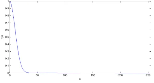
Since the aim is to interpolate along edges and not across them, an inverted gradient function is formed:

f_grad(x) =      1 x i f x̸= 0 1 i f x = 0 (1.17)

where x represents one of the gradient of (1.16). This function allows to weight more the smallest gradients and to follow the edge orientation. The interpolation of missing luminance values is performed using the normalized inverted gradient functions which weight both luminance and chrominance values in the neighbor-hood. The chrominance values are used in the interpolation of luminance to get a more accurate estimation. Similarly, chrominances are interpolated by using both luminance and chrominance data. The correction step comprises the lumi-nance correction first, and then the chromilumi-nance correction.

The method in [105] aims to generate images with sharp edges. And also in this case a high frequency component, derived from the sensed color channel, is added to the low frequency component of the interpolated channels. This tech-nique takes into account eight different directions, as it shown in Fig.(1.7), and uses 5× 5 elliptical Gaussian filters to interpolate the low frequency component

of each color channel (even the sensed one). For each available direction there is a different Gaussian filter, having the greater coefficients along the identified di-rection. These filters have the advantage of interpolating the missing information without generating annoying jaggy edges.

8 5π 4 3π 8 7π 2 π 4 π 8 3π 8 π 0

Figure 1.7 : Quantized directions for spatial gradients.

After having computed the low frequency component, for each color channel, an enhancement of the high frequencies content is obtained taking into account the color correlation (1.22). In particular, a correction term is calculated as the difference between the original sensed value and its low pass component, as it is retrieved through the directional Gaussian interpolation:

∆Peak= G− GLPF (1.18)

This correction term is then added to the low frequency component of the chan-nels to be estimated:

H = HLPF+∆Peak (1.19)

The low frequency component, in this method, is calculated according to the identified direction, so it is less affected by false colors than previous inventions. Moreover, this solution provides a simple and effective method for calculating

direction and amplitude values of spatial gradients, without making use of a first rough interpolation of the G channel. More specifically, 3× 3 Sobel operators are applied directly on the Bayer pattern to calculate horizontal and vertical gra-dients. The orientation of the spatial gradient at each pixel location is given by the following equation:

or(x, y) =          arctan ( P′∗ Sobely(x, y) P′∗ Sobelx(x, y) ) if P′∗ Sobelx(x, y)̸= 0 π 2 otherwise (1.20)

where P′∗ Sobely and P′∗ Sobelx are the vertical and horizontal Sobel filtered

values, at the same pixel location. The orientation or(x, y) is quantized in eight predefined directions. Since the image could be deteriorated by noise, and the calculation of direction could be sensitive to it, a more robust estimation of di-rection is needed. For this reason, Sobel filters are applied on each 3× 3 mask within a 5× 5 window, thus retrieving nine gradient data. In addition to the orientation, the amplitude of each spatial gradient is calculated, by using the following equation:

mag(x, y) =(P′∗ Sobel_x(x, y))2+(P′∗Sobel_y(x, y))2 (1.21)

The direction of the central pixel is finally derived through the “weighted-mode” operator, which provides an estimation of the predominant amplitude of the spa-tial gradient around the central pixel. This operator substanspa-tially reduces the effect of noise in estimating the direction to use in the interpolation phase.

Spectral Correlation Based Approaches

In this class of algorithms final RGB values are derived taking into considera-tion the inter-channel color correlaconsidera-tions in a limited region. Gunturk et al. [65] has demonstrated that high frequency components of the three color planes are highly correlated, but not equal. This suggests that any color component can help to reconstruct the high frequencies for the remaining color components. For in-stance, if the central pixel is red R, the green G component can be determined as:

G(i, j) = GLPF(i, j) + RHPF(i, j) (1.22)

where RHPF(i, j) = R(i, j)− RLPF(i, j) is the high frequency content of the R

channel, and GLPF and RLPF are the low frequency components if the G and R

channels, respectively.

This implies that the G channel can take advantage of the R and B information. Furthermore for real world images the color difference planes (∆GR = G− R

and∆GB= G− B) are rather flat over small regions, and this property is widely

exploited in demosaicing and antialiasing techniques. This model using chan-nel differences (that can be viewed as chromatic information), is nearer to the Human Color Vision system that is more sensitive to chromatic changes than luminance changes in low spatial frequency regions. Like the previous example, if the central pixel is R, the green component can be derived as:

G

G

G

G

G

G

G

G

G

G

Figure 1.8 : Pattern of five pixels used to calculate an edge metric on a central G pixel of the LF (low frequency) G color channel.

The method proposed in [80] belongs to this class. The technique generates by first an estimation of all color channels (R, G and B) containing the Low Frequencies (LF) only. This is obtained by taking into consideration an edge strength metric to inhibit smoothing of detected edges. Then a difference be-tween the estimated smoothed values and the original Bayer pattern values is performed to obtain the corresponding High Frequency (HF) values. Finally the low frequency channels and the corresponding estimated high frequency planes are combined into the final RGB image. In particular the high frequency values are obtained through the relations described in Table.1.1.

Table 1.1 : Color Correlations defined in [80]. At a Red Pixel At a Green Pixel At a Blue Pixel

R R RLPF+ G− GLPF RLPF+ B− BLPF

G GLPF+ R− RLPF G GLPF+ B− BLPF

B BLPF+ R− RLPF BLPF+ G− GLPF B

Each smoothed LF image is formed by a two-dimensional interpolation com-bined with a low-pass filtering excepted for pixels that maximize the edge strength metric. For example, if the central pixel is a G pixel the four adjacent G pixels, which will be taken into consideration to estimate the edge strength, are gen-erated by interpolation (see Fig.(1.8)). Thus the measure of edge strength Ei j,

according to:

Ei j= (Gi, j− Gi, j−1)2+ (Gi, j− Gi, j+1)2+ (Gi, j− Gi−1, j)2+ (Gi, j− Gi+1, j)2

(1.24) By considering this edge metric the algorithm reduce the presence of color arti-facts on edges boundaries.

In [35] a method based on the smooth hue transition algorithms by using the color ratio rule is proposed. This rule is derived from the photometric image for-mation model, which assumes the color ratio is constant in an object. Each color channel is composed of the Albedo multiplied by the projection of the surface normal onto the light source direction. The Albedo is the fraction of incident light that is reflected by the surface, and is function of the wavelength (is differ-ent for each color channel) in a Lambertian surface (or even a more complicate Mondrian). The Albedo is constant in a surface, then the color channel ratio is hold true within the object region. This class of algorithms, instead of us-ing inter-channel differences, calculates the green channel usus-ing a well-known interpolation algorithm (i.e., bilinear or bicubic), and then computes the other channels using the red to green and blue to green ratios, defined as:

Hb=

B

G and Hr= R

G. (1.25)

An example of such method is described in [111]. In this work the Bayer data are properly processed by a LPF circuit and an adaptive interpolation module. The LPF module cuts off the higher frequency components of the respective color signals R, G and B and supplies RLPF, GLPF and BLPF. On the other hand, the

signals R and G and executes interpolation with a pixel which maximizes the correlation to obtain a high resolution luminance signal.

_R

_G

_R

G

G

R

G

R

G

G

G

G

R

G

R

G

G

R

G

R

G

G

G

G

Figure 1.9 :RG pixel map for luminance interpolation.

The authors assume that, since the color signals R and G have been adjusted by the white balance module, they have almost identical signal levels and thus they can be considered as luminance signals. Taking into consideration the Bayer pattern selected in Fig.(1.9), they consider the luminance signals arranged as shown in Fig.(1.10), where the value Y5 has to be calculated according to the

surrounding values.

The correlation S for a set of pixels Ynalong a particular direction can be defined,

similarly to the (1.25), as follows:

S = min(Yn) max(Yn)

(1.26)

where S≤ 1 and the maximum correlation is obtained when S = 1.

The correlation is calculated for the horizontal, vertical and diagonal directions, and interpolation is executed in a direction which maximizes the correlation. For instance, for the vertical direction:

and

max(Yn) = max(Y1,Y4,Y7)· max(Y2,Y8)· max(Y3,Y6,Y9) (1.28)

The correlations in the horizontal and diagonal directions are computed in a similar way. If the direction which maximizes the correlation is the vertical one, the interpolation is executed as follows:

Y5=

(Y2+Y8)

2 (1.29)

Another way to decide the direction is to consider the similarities between the pixels. The dispersion degreeσR of the color R is calculated as:

σR=

min(R1, R2, R3, R4)

max(R1, R2, R3, R4)

(1.30)

If the dispersion degree is greater than a threshold, interpolation along a diagonal direction is executed. On the contrary, when the dispersion degree is small, correlation of the color R is almost identical in any directions, so it is possible to interpolate only G along the vertical or horizontal direction. This implies that the interpolation is executed only with G having the highest frequency, thus enabling to obtain an image of a higher resolution.

Once the luminance signal Y is interpolated, a high pass filter (HPF) is applied to Y and the color signal R and G. The HPF creates a luminance signal YHPF

containing higher frequency components only. Finally, an adder combines the already computed color signals RLPF, GLPF and BLPF with the higher frequency

_Y

_Y

_Y

_Y

Y

Y

Y

Y

Y

Figure 1.10 :Luminance map of analyzed signal.

Non Adaptive Approaches

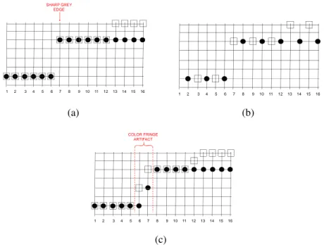
The pattern based interpolation techniques perform, generally, a statistical anal-ysis, by collecting actual comparisons of image samples with the corresponding full-color images. Chen et al. [34] propose a method to improve the sharpness and reduce the color fringes with a limited hardware cost. The approach consists of two main steps:

1. Data training phase:

(a) Collecting samples and corresponding full-color images;

(b) Forming pattern indexes, by selecting the concentrative window for each color in the Bayer samples and quantizing all the values on the window;

(c) Calculating the errors between the reconstructed pixels and the actual color values;

(d) Estimating the optimal combination of pattern indexes to be sorted into a database.

2. Data practice phase:

(a) For each pixel a concentrative window is chosen, and within it, the pixels are quantized in two levels (Low, High) to form a pattern index,

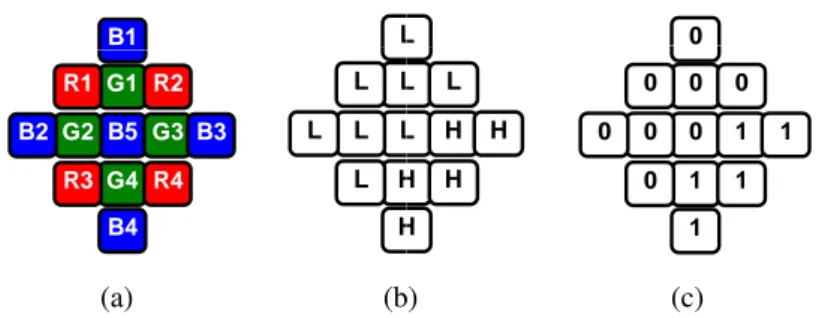
as shown in Fig.(1.11). This index is then used as key for the database matching. B1

Figure 1.11 : Relationship between a color filter array and a concentrative win-dow. (a) Bayer Pattern, (b) Quantization of acquired samples in two levels: Low (L) and High (H), (c) Resulting pattern index.

During the data training phase, the proposed method assumes that the recon-structed value (Recvalue) is function of the original value (Origvalue) and the

feasible coefficient set ( f easible coe f f icient set), which can be expressed as:

Recvalue=

Origvalue∗ f easible coe f ficient set

(sum o f coe f f icients) (1.31) Once the value has been calculated for each f easible coe f f icient set, the sys-tem chooses the set having the minimal error between the calculated values and the real value. These results are then stored into the database. During the data-practice phase, the reconstruction is based on color differences rules applied to the pixel neighborhood.

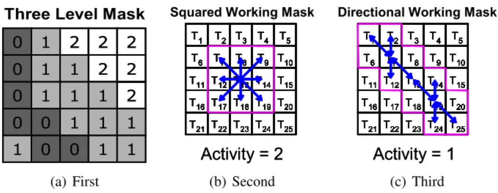
A simpler technique [86] uses a plurality of stored interpolation patterns. To se-lect the correct interpolation pattern an analysis of the input signal is performed using gradient and uniformity estimation. In practice, by first the G channel is interpolated using the 8 stored fixed patterns (Horizontal, Vertical, the two Di-agonals and the four corners). To achieve this purpose the uniformity and the

gradient are estimated in the surrounding of the selected G pixel. The minimum directional data estimation Gv(i) (i∈ [1..8]) , obtained through the eight fixed

patterns, defines the best match with the effective direction.

For example, Fig.(1.12.(a)) shows an interpolation pattern in which low lumi-nance pixels are arranged along the diagonal.

G11 Q21 G31 Q41 G51

Figure 1.12 :Some samples of interpolation patterns.

The directional data Gv(1), which represents a numerical value of the similarity

between the surround of the pixel to be interpolated and the interpolation pattern, is obtained through the following expression:

Gv(1) = |G33− G51| + |G33− G42| + |G33− G24| + |G33− G15|

4 (1.32)

The remaining seven directional data are calculated in a similar manner, tak-ing into account the fixed direction. The smallest directional data from Gv(1)

to Gv(8) identifies the interpolation pattern which is the best fit to the image

neighborhood of the pixel to be interpolated.

When one interpolation pattern only is present, providing the smallest direc-tional value, it is chosen to perform the interpolation. On the contrary, when two or more interpolation patterns provide the smallest directional value, a

correla-tion with the interpolacorrela-tion patterns of the surrounding pixels, whose optimum interpolation pattern has already been determined, is considered.

Specifically, if one of the interpolation patterns having the smallest value is the interpolation pattern of one surrounding G pixel, this pattern is chosen for per-forming the interpolation. Otherwise it is impossible to determine a specific pattern to use for the interpolation, and thus a simple low pass filter is applied. If Gv(1) is the smallest directional value:

G0 = G15+ 2G24+ 2G33+ 2G42+ G51 8 (1.33) P0 = P14+ P34+ P32+ P52 4 (1.34) Q0 = Q23+ Q25+ Q43+ Q41 4 (1.35)

where P and Q represent the R and B or B and R values. If it is impossible to determine a specific pattern:

G0 = (G22+ G24+ G42+ G44+ 4G33) 8 (1.36) P0 = (P34+ P32) 2 (1.37) Q0 = (Q23+ Q43) 2 (1.38)

Once the missing values for the G pixels have been processed, the algorithm cal-culates the missing values for the R and B pixels. If the interpolation patterns, estimated for the already processed G pixels, describe a fixed direction in the surrounding of the R/B pixel (that is several patterns indicate the same direction) then this pattern is used to perform the interpolation. Otherwise the numerical directional data are estimated. Like the G case, eight different interpolation pat-terns are stored in the interpolation storage memory and a directional data value

is computed for each of these patterns. When there are two or more patterns having the smallest directional data value, correlations with the interpolation patterns of the already interpolated G pixels are evaluated. The reason why G pixels are taken into consideration instead of R and B pixels is that G pixels are more suitable for pattern detection than R and B pixels.

This class of techniques is very robust to noise, because it takes into consider-ation the interpolconsider-ation patterns of the already processed pixels, but introduces jagged edges in abrupt diagonal transitions, due to the equations used in the interpolation step.

Iterative Approaches

In this category we collect all approaches that derive interpolation through an iterative process able to find after a limited number of cycles the final mosaicized image. In particular, in [70, 71, 83], starting from an initial rough estimate of the interpolation, the input data are properly filtered (usually using a combination of directional high-pass filters with some global smoothing) to converge versus stable conditions. These methods proceed in different ways with respect to the local image analysis but share the overall basis methodology.

In [83] a color vector image is formed containing the original Bayer values. Af-ter an initial estimate of the RGB original value for each pixel such quantity is updated by taking into account two different functions: “roughness” and “pre-ferred direction”. The final missing color are defined by finding the values that minimize a weighted sum of Rough and CCF (Color Compatibility Function)

functions over the image by using the following formula: Q =

∑

∑

whereλ is a positive constant while Rough(m, n) is defined in this case as the lo-cal summation of approximated lolo-cal gradients and CCF(m, n) is a function that penalizes local abruptly changes. By using the classic Gauss-Siedel approach the method converges after 4-5 iterations.

In [70] and [71] the luminance channel is properly extracted from input Bayer data and analyzed in a multiscale framework by applying smoothing filtering along preferred directions. Chrominance components are smoothed by isotrop-ically smoothing filters. The final interpolated image is obtained after a few iterations. Just before to start a new iteration the pixel values are reset to the original (measured) values.

1.1.2

Frequency-domain Approaches

Demosaicing is an ill posed problem and thus it cannot have a unique solution. This can be easily understood by considering that different real images can have the same mosaiced representation [8]. The mosaicing operation cannot be in-verted and thus, it necessary to consider a priori assumptions to extrapolate the missing information. All the demosaicing algorithms use specific a priori as-sumptions to design the interpolator operator. One of the a priori assumption is the band limited of image signal and the limit is due to the sampling rate of the color channels.

In natural images, the energy spectrum is primarily present in a low frequency region and high frequencies along the horizontal and vertical axes [49], and the

human visual system is more sensitive to these high frequencies than to the ones present at the corner of the spectrum. The demosaicing algorithms in the fre-quency domain exploit these band limit assumptions.

Fourier Transform Analysis and Processing

Several demosaicing algorithms in the Fourier domain have been proposed in literature [59, 76, 77] exploiting the spectrum properties of the CFA mosaiced images. The spectral representation of a CFA image can be directly derived from its representation in the spatial domain.

A color image I can be represented as:

I (x, y) ={Ci(x, y)},i ∈ {R,G,B},(x,y) ∈ N2 (1.40)

where Ciare the color vectors in the lattice (x,y). Thus an image is expressed as

a vector of three dimensions for each pixel. The color triplets Ci form a linear

vector space of three dimensions. If we call ICFAthe spatial multiplexed version

of the image I with a CFA pattern, we have: ICFA(x, y) =

∑

i∈{R,G,B}

Ci(x, y)· Di(x, y) (1.41)

where Di(x,y) are the sampling functions that have value 1 if the color channel is

present at the location (x,y), or 0 if not present. In case of the Bayer arrangement of CFA, the Di represent the disjoint shifted lattices and can be expressed in

terms of cosine modulation: DR(x, y) =

1

4(1 + cos (πx)) (1 + cos (πy)) DG(x, y) =

1

2(1− cos(πx) cos (πy)) DB(x, y) =

1

4(1− cos(πx)) (1− cos(πy))

The mosaiced image ICFA in the Fourier domain is the Fourier transform of the (1.41): ˆ ICFA(u, v) =

∑

Ci(u, v)∗ ˆDi(u, v) = ˆRCFA(u, v) + ˆGCFA(u, v) + ˆBCFA(u, v)

(1.43) where∗ denotes the convolution operator, the ˆ. represents the Fourier Transform,

ˆ

RCFA, ˆGCFA and ˆBCFA are Fourier Transform of the sub-sampled color

compo-nents. The modulation functions defined in (1.42) are based on cosine and have their Fourier Transform expressed in Dirac. These transforms can be compactly arranged in a matricial form:

ˆ Di(u, v) =∆(u)TM3x3∆(v) (1.44) where ∆(u)=[ δ(u + 0.5) δ(u) δ(u− 0.5) ]T and ∆(v)=[ δ(v + 0.5) δ(v) δ(v− 0.5) ]T

As expressed in (1.43), the Fourier Transform of the sub-sampled color channels can be derived by convolving the original ˆCi channels with the corresponding

modulation functions Di(x,y); making the matrices of (1.44) explicit:

ˆ

RCFA(u, v) = ˆCR(u, v)∗

 ∆(u)T   − 1 16 1 8 − 1 16 −1 8 1 4 − 1 8 −1 16 1 8 − 1 16  ∆(v)   ˆ

GCFA(u, v) = ˆCG(u, v)∗

 ∆(u)T   1 8 0 1 8 0 1₂ 0 1 8 0 1 8  ∆(v)   ˆ

BCFA(u, v) = ˆCB(u, v)∗

 ∆(u)T   − 1 16 − 1 8 − 1 16 1 8 1 4 1 8 −1 16 − 1 8 − 1 16  ∆(v)   (1.45)

This matrix representation is useful because it clarifies how the samples are scaled replications of the Fourier transform of the full resolution channels. The

ˆ

GCFA formula in (1.45) points that the replications are placed on the diagonal

directions only, while the ˆRCFA and ˆBCFA have replications also on the

horizon-tal and vertical directions. The Fig.(1.13) shows the Fourier transform of the sub-sampled green channel and of the red and blue channels. In Fig.(1.13(b)) the spectrum of the whole ICFAis shown. It is evident the overlapping among the

base band and the shifted replication, that is the cause of color artifacts.

To overcome the aforementioned overlapping, Alleysson [10] started from the commonality between the human visual system (HVS) and the CFA based im-age sensors to sample one color only in each location (that is a pixels for imaging devices, a cone or a rod for the human eye) and thus spatial and chromatic in-formation is mixed together. It is also known that the HVS encode the color information into luminance and opponent color signals. Similarly, for CFA sen-sors each color sample is composed by a spatial information due its position and chromatic information due to its spectral sensitivity. According to this represen-tation, the (1.40) can be rewritten as:

I (x, y) ={Ci(x, y)} =ϕ(x, y) +{ψi(x, y)} =

∑

pi·Ci(x, y) +{ψi(x, y)}

(1.46) The spatial information, expressed by the scalar termϕ, is composed by a weighted sum of each color channel, while{ψi} is a vector of three opponent color

com-ponents. Subtracting the luminance to the color image, the chrominance infor-mation is obtained. For CFA images the modulation functions can be rewritten as composed by a constant part piand by a fluctuation part with null mean ˜Di:

(a) Input image. fy 1/2 0 1/2 -1/2 0 -1/2 0 I bp M Max 1/2 0 f 0 1/2 0 fx

(b) Global CFA Spectrum.

fy 1/2 0 1/2 -1/2 0 -1/2 0 R M Max 1/2 0 f 0 1/2 0 fx (c) RB original Spectrum. fy R 1/2 0 1/2 -1/2 0 -1/2 0 R bp M Max 1/2 0 f 0 1/2 0 fx (d) RB CFA Spectrum. fy 1/2 0 1/2 -1/2 0 -1/2 0 G M Max 1/2 0 f 0 1/2 0 fx

(e) G original Spectrum.

fy G 1/2 0 1/2 -1/2 0 -1/2 0 G bp M Max 1/2 0 f 0 1/2 0 fx (f) G CFA Spectrum.

The pi represent the probability of presence of each color channel in the CFA.

Since in the Bayer pattern the green components are twice the red and blue pix-els, then pR= 1₄, pG= ₂1 and pB = 1₄. According to the (1.41) the ICFA is now:

ICFA(x, y) =

∑

pi·Ci(x, y) +

∑

Ci(x, y)· ˜Di(x, y) (1.48)

The first term represents the luminance and the second vectorial term represents the chromatic components. this representation highlights how the luminance term in (1.48) is the same of (1.46), that is the luminance in CFA images is ex-actly present and not subjected to interpolation even if it is subjected to aliasing with chrominances. Thus a good estimation of luminance information is fun-damental. The localization of luminance is performed on the Fourier domain. Exploding the (1.43) with the equations in (1.45), it easily to rewrite ˆICFAas:

ˆ ICFA(u, v) =

∑

∑

∑

∑

∑

∑

∑

where ˆL(u, v) is the luminance, ˆC1(u, v) and ˆC2(u, v) are the chrominance, the

(1.49) becomes:

ˆ

ICFA(u, v) = ˆL (u, v) + ˆC1(u, v) + ˆC2(u, v) (1.51)

The relations in (1.50) can be expressed in matricial form:   _CˆˆL (u, v)_{1(u, v)} ˆ C2(u, v)   =   1 4 1 2 1 4 −1 4 1 2 − 1 4 −1 4 0 1 4   ·   ˆ CR(u, v) ˆ CG(u, v) ˆ CB(u, v)   (1.52)

The inverse of this matrix represents the relation between the RGB values in the CFA image and the luminance/chrominance signals in the Fourier domain.

fy 1/2 0 1/2 -1/2 0 -1/2 0 L M Max 1/2 0 f 0 1/2 0 fx

Figure 1.14 :Luminance Spectrum.

The spectrum of ˆL(u, v) is not shifted, ˆC1(u, v) is located at the corner of the

spectrum, while ˆC2(u, v) is located at the sides of the spectrum, as shown in

Fig.(1.14) and Fig.(1.15). The smoothness of the color difference channels im-plies a more limited band for ˆC1(u, v) and ˆC2(u, v) and, consequently, the

replica-tion are more compact and less overlapping than the R and B subsampled chan-nels. This allows to design better performing filters to discriminate luminance from the shifted bands than in the R, G and B representation.