Università degli Studi di Salerno
DIPARTIMENTO DISCIENZEECONOMICHE ESTATISTICHE
Marialuisa Restaino1
D
ROPPING OUT OFU
NIVERSITY OFS
ALERNO:
A
SURVIVAL APPROACHWORKINGPAPERn. 3.193
1
Dipartimento di Scienze Economiche e Statistiche, Università di Salerno, Italy, Email:[email protected]
Contents
1 Introduction . . . . 7
2 Background and existing works on university dropout event . . . . 9
3 The student level data of the University of Salerno . . . 12
4 Statistical framework of Survival Analysis . . . 19
5 Analysis of the dropout rates at the University of Salerno . . . 28
Abstract
The aim of this paper is to analyse and model the interval of time between the first enrolment at University and the first occurrence of non-enrolment, so that the event of interest is the dropping out of University. The interest is focused on computing the probability of surviving at the University and analysing which personal, familiar and social characteristics may influence the non-completion of students’ academic carrier, using Survival Analysis techniques. The dataset analysed is collected from the Central Administra-tive Office of the University of Salerno, and includes all full-time students enrolled at the 2002-2003 academic year, followed for five years, until the 2006-2007 academic year. Those students can either complete their study and receive their degree or leave the university, that is the event of our in-terest. The estimation of the probability of surviving in University is made by the Kaplan-Meier estimator. Then, to test if there is a significant difference among the survival curves, Log-rank test is considered. Since it does not allow more than one explanatory variable to be taken into account, Cox Pro-portional Hazards model is used to analyse the interrelations between the covariates, and explored the influence of covariates on failure times. This study shows that there is a steep decline for students in Political Science and in Educational Studies, at the first year. Moreover, female students, stu-dents who attended "Licei" and those who completed their high school study with the highest mark (i.e. 110) have the highest probability of surviving at the University, i.e. the highest rate of taking the degree. In all these cases, it can be noted that there is a Faculty effect. These differences, tested by log-rank test, are significant. Finally, Cox PH model for each Faculty confirms previous results.
Keywords
Dropout, Kaplan-Meier Estimator, Log-rank Test, Cox Proportional Hazards Model.
1 Introduction
University dropout is an important topic in many countries, since the high rates of dropouts mean waste of public money, a lower proportion of grad-uated people and consequently lower employment opportunities in highly qualified position.
There are two possible definitions of university dropouts. The first defini-tion refers to college students leaving a college in which they are registrered, while the second one associates dropout with those who never receive a col-lege degree (Spady, 1970). In this paper, dropout is defined as a student who registered for a degree programme, but does not complete it. The first definion cannot be used since the exact date in which the students leave the university, is unknown.
In literature several factors are associated with student dropout in higher education institutions (Astin, 1964; Bayer, 1964; Spady, 1970; Tinto, 1975). Those factors can be divided into two categories: factors associated with attributes or characteristics of the individual student, and those associated with the institutional environment.
Since there are so many different alternative factors which can affect the non-completion of study, it is crucial to study and analyse which ones are relevant to explain the non-completion event in institutions of higher educa-tion (Johnes, 1990; Checchi et al., 1999; Arulampalam et al., 2005).
For this purpose, two models are usually used: Student Integration
Model (Tinto, 1975) and Student Attrition Model (Bean, 1980, 1982).
The first focuses on the importance of students’ academic and institu-tional commitments, derived by interrelations that take place within the
in-stitution, namely a matching between students’ motivations and academic ability and academic and social characteristics.
The second model, instead, emphasizes the importance of the inten-tion to remain enrolled or to depart from college. According to this model, factors external to the institution are those which influence student attitudes and enrolment decisions.
Though both models analyse the departure from the university in com-peting framework, Cabrera et al. (1993) points out that it is possible to over-lap the two models, developing an integrated model that yields a different view of the persistence process. They highlight how not only social, per-sonal and academic factors, but also psycological and sociological elements influence the student decision of leaving the University.
In these models, the timing of the different ways in which students can exit higher education (stopout, dropout, transfer, academic dismissal, grad-uation) is ignored. In order to take into account the timing of departure pro-cess, Event-history models are considered (DesJardin et al., 1999, 2006; Ishitani, 2003; Kalamatianou and McClean, 2003; Johnson, 2006).
Event-history modeling is a longitudinal analytic technique that is partic-ularly well suited to study the temporal nature of student academic careers. This technique allows to evaluate transitions from one state to the next, i.e. from being enrolled or not, and to incorporate variables that capture the changing circumstances faced by students, as they proceed through their academic careers. It is important to study student academic careers us-ing longitudinal data and temporal analytic techniques, because other tech-niques, like cross-sectional models, do not include temporal information and therefore they cannot be used to explain how changes in independent vari-ables affect changes in the object of interest. In fact, cross-sectional designs are only concerned with how levels of explanatory variables explain an out-come at a specific point in time. Moreover, by using cross-sectional data and static methods to study temporal processes, it is difficult to establish the direction of casuality. Thus, if the purpose of the analysis is to explain change, longitudinal techniques, like event-history modeling, are preferred to static, cross-sectional designs.
The aim of this paper is to analyse and model the interval of time be-tween the first enrolment at the University and the first occurrence of
non-enrolment, so that the event of interest is the dropping out of the Univer-sity. The interest is focused on analysing which personal, familiar and social characteristics may influence the non-completion of students’ academic car-rier at the University of Salerno by using Survival Analysis techniques.
The paper proceeds as follows. Section 2 describes the background and the existing works on university dropout process, discussing on one hand which models are used in literature for analysing the dropout process, and on the other hand, which factors may influence the students’ decision of leaving the university. Section 3 introduces the models used in this paper, to analyse the probability of dropping out of university. In particular, Survival Analysis techniques are discussed, considering three statistical tools: the Kaplan-Meier Estimator, for estimating the survival probability, the Log-Rank Test, for comparing two or more survival curves, according to some covari-ates, and the Cox Proportional Hazards Model, for identifying which ele-ments might influence the decision of dropping out of the university. Then, a description of student level data, used for estimating the probability of sur-viving at the university, is given in Section 4, and the results of the analyses are reported and discussed in Section 5. Some concluding remarks close the paper.
2 Background and existing works on university dropout event
There are many studies that investigate the determinants of university dropout event, using student level data. The general idea is that personal, familiar and institutional characteristics may influence the decision of leav-ing university without completleav-ing the program of study.
In the past, two theoretical models have been developed: Student
Inte-gration Model (Tinto, 1975) and Student Attrition Model (Bean, 1980, 1982).
The assumption of the first model is that the completion of University study depends on interaction between students and learning environment. In other words, the way in which motivation and academic ability of stu-dents iteract with the academic and social characteristics of universities, influences the chance of completing the program. Thus, students who do not interact with other undergraduates on campus or have negative
experi-ences, might decide to leave the university.
The assumption of second model is that student non-completion is silar to a turnover in work organizations and the behavior intentions are im-portant predictors of persistence behavior. The central point of this model is that students come to university with certain attitudes and expectations that are confirmed or disproved through campus experiences. Undergraduates either confirm the initial expectations or form new impressions, depending on the interactions with their peer. Student intentions of leaving are found to be predictive of actual leaving behavior. This model is expanded to take into account student background characteristics that are related to integration. Therefore, organizational, personal and environmental variables influence the attitudes, the intents and the decision of leaving or continuing study.
Even though these models examine the departure from college as a lon-gitudinal process, in which students’ decision to continue studying is influ-enced by the quality of interactions between precollege characteristics and institutional environments, they consider the departure process in a com-peting framework. However, it might be interesting to merge these models, developing an integrated model, through the structural equation modeling (Pascarella and Chapman, 1983; Braxton, Duster and Pascarella, 1988; Cabrera, Nora and Castaneda, 1993). In this way, students’ dropout behav-ior is described, pointing out that academic and social factors influence the decision of non-completion of study, but in this model time timing of dropout is not considered.
The role of time in dropout studies is analysed, using the Event-History model (DesJardin et al., 1999, 2006; Ishitani, 2003; Kalamatianou and Mc-Clean, 2003; Johnson, 2006), in order to focus on the time periods when students are at risk of leaving the institution, identifying which character-istics affect the probability of dropping out. This technique is particularly interesting for analysing the departure process, because the assessment of the transition from one state to another, i.e. from enrolled to not enrolled, and the identification of the factors (personal, academic, familiar) which in-fluence the students’ decision of leaving, are attainable.
Among the several determinants that might influence the chance of study non-completion, dropout risk is associated with the topic studied at univer-sity and pre-college academic qualification. In other words, the probability
of dropping out of university is higher among students with relatively poor levels of prior qualifications (Johnes, 1990; Light ans Strayer, 2000; Smith and Naylor, 2001; Arulampalam et al., 2005). The likelihood of withdrawing tends to be higher among students in the science disciplines, such as math-ematics, engineering and technology and physical science (Johnes and Mc-Nabb, 2004).
Completion rates may also vary across gender and age. In particular, males and more mature students are more likely to drop out compared to females or youger students, respectively (Bean and Metzner, 1983; Arulam-palam et al., 2004).
In addition to individual characteristics, several institution-specific fac-tors are also found to affect university completion, such as the gender com-position of faculty and institutional quality, measured by the results of subject-specific Teaching Quality Assessment (TQA). In detail, students attending universities characterised by high standards of quality in teaching have a lower probability of dropping out relative to those studying at universities that do not achieve the same standards (Robst et al., 1998; Johnes and McNabb, 2004).
Furthermore, working when attending school reduces educational at-tainment. One explanation suggested is related to the fact that students who work have less time for doing other activities, including studying (Eck-stein and Wolpin, 1999).
Parental income, education and socio-economic status are generally im-portant determinants of individual education choices and of the probability of graduation. Empirical evidence on income and occupational mobility sug-gests that university graduates mainly come from higher educated families (Eckstein and Wolpin, 1999; Checchi et al., 1999; Cingano and Cipollone, 2003; Checchi and Flabbi, 2006).
Finally, a reduction in higher education standards goes in the direction of increasing the number of students in tertiary education and also, by re-ducing dropout, the graduation rates (Di Pietro and Cutillo, 2006; Bratti et
al., 2007).
Some studies have concentrated on the hypothesis that the Italian Uni-versity Reform, according to the Law 509/99, might have reduced both stu-dents’ workloads and grading standards in exams. Di Pietro and Cutillo
(2006), focusing on impact of the Italian University Reform on dropout rates, use a decomposition methodology to assess whether changes in the prob-ability of dropping out are determined by changes in students’ observable characteristics or by changes in students’ behaviour. Their findings suggest that since students’ characteristics worsen after the reform, i.e. they tend to achieve poorer academic outcomes, which in turn result in higher dropout rates, the reduction in dropout rates could be explained by a change in stu-dent behaviour, such as higher motivation to complete a study program, better focused and more labour market oriented curricula, increased possi-bilities to combine study and work.
Bratti et al. (2006) look into the hypothesis that the fast increase in the number of students is accompanied by a reduction in the higher education and investigates the consequences on drop out and graduation rates. They illustrate a case study on the Marche Polytechnic University, reporting a significant reduction in course workloads and an increase in student perfor-mance after the reform, which are shown to have significantly reduced the likelihood of student dropping out.
3 The student level data of the University of Salerno
The dataset is collected by the Central Administrative Office of the versity of Salerno, and includes all full-time students enrolled at the Uni-versity in the 2002-2003 academic year. They have been followed for five years, until the 2006-2007 academic year. Those students can have two status: they complete their study, taking the degree or they leave the univer-sity, that is the event of our interest.
In this paper, an individual is assumed to have successfully completed his/her study, if he/she takes the degree by the end of third year. Dropout is, therefore, defined as withdrawal from his/her degree programme.
The duration of time is five years (the regular duration of study, i.e. 3 years, plus two additional years). At the end of the fifth year, it is assumed to be a forced termination: a successful completion or dropout. Moreover, since there is no available any information about the following academic
year (2007/2008), it is assumed that students who are still enrolled at the beginning of the fifth year, may continue their study in the next academic year, and they do not leave their study.
For each subject, some covariates have been registered, as shown in Table (3.1). The Law Faculty is not considered, because marks of exams are missing in the dataset.
Variable Name Definitions
Faculty the study programme chosen by student
(Economics; Pharmaceutics; Engineering; Humanities; Languages; Educational Studies; Mathematical, Physical and Natural (MFN) Sciences; Political Science)
Year of enrolment Last Year of study attended by student Gender 1 if the student is Female, 0 if Otherwise Age Age at the time of enrolment,
divided into four classes (18-19; 20-21; 22-23; >24) School Attended High School attended by student before enrolling
(Classical, Scientific, Technical, Professional, Langagues, Training, Professional, Others) High school final mark Mark of the final exam of High School,
divided into classes (60-69; 70-79; 80-89; 90-99; 100) Income Family Income level
(range: from 1 if the level is low, to 9 if the level is high) Average mark of exams Mean of exams’ marks of student,
divided into classes (18-21; 22-24; 25-27; 28-30)
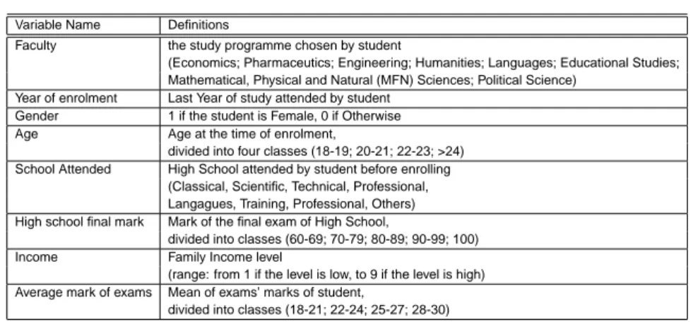
Table 3.1: Description of the characteristics registered for the students. The population analysed consists of 5823 full-time students, enrolled in 2002-2003 academic year at the University of Salerno. The Table (3.2) shows the distribution of population, by Faculty and Gender. It can be noted that female students choose to study Educational Studies (96
%
), Lan-guages (82%
), Pharmaceutics (70%
) and Humanities (68%
), while the other Faculties have typically a male setting.Faculty Female Male Total Economics 507 (0.48) 551 (0.52) 1058 (0.18) Pharmaceutics 308 (0.70) 132 (0.30) 440 (0.08) Engineering 129 (0.20) 532 (0.80) 661 (0.11) Humanities 962 (0.68) 458 (0.32) 1420 (0.24) Languages 358 (0.82) 80 (0.18) 438 (0.08) Educational Studies 569 (0.91) 55 (0.09) 624 (0.11) MFN Sciences 197 (0.24) 621 (0.76) 818 (0.14) Political Science 136 (0.37) 228 (0.63) 364 (0.06) Total 3166 (0.54) 2657 (0.46) 5823
Table 3.2: Distribution of male and female, for Faculty in which they are
enrolled. (The percentage values are given in parentheses.)
Though in Italy, the normal age of entry into the University is 18-19 years, the average age at time of the enrolment at the University of Salerno is 20-21 for all Faculties, with the exception of Political Science, for which students are older (23 years, in average). Moreover, most of the Facul-ties have a lower percentage of students with more than 24 years, whereas these rates are rather higher for Political Science (20
%
) and Educational Studies (14%
) (Table (3.3)).Faculty 18-19 20-21 22-23 >24 Economics 649 (0.61) 295 (0.28) 39 (0.04) 75 (0.07) Pharmaceutics 292 (0.66) 101 (0.23) 11 (0.03) 36 (0.08) Engineering 498 (0.75) 119 (0.18) 14 (0.02) 30 (0.05) Humanities 804 (0.57) 409 (0.28) 67 (0.05) 140 (0.10) Languages 283 (0.65) 114 (0.26) 19 (0.04) 22 (0.05) Educational Studies 317 (0.51) 174 (0.28) 43 (0.07) 90 (0.14) MFN Sciences 495 (0.61) 228 (0.28) 38 (0.05) 57 (0.07) Political Science 155 (0.43) 111 (0.31) 22 (0.06) 76 (0.20) Total 3493 (0.60) 1551 (0.27) 253 (0.04) 526 (0.09)
Table 3.3: Distribution of students, for Faculty and Age at time the enrolment.
(Percentage values are given in parentheses.)
The distribution of population, distinguishing among types of high school is shown in Table (3.4). In Italian High School System, there are several types of high schools, which can be divided into three different categories: "Licei", i.e. classical, scientific and linguistic high schools, "Technical", tech-nical and professional schools, and "Others", including other types of high schools, and schools not specified by the students.
Students who attended "Licei" prefer to enrol in Pharmaceutics (70
%
), Humanities (67%
), Languages (63%
), Educational Studies (65%
) and Engi-neering (57%
), whereas students who attended Technical High school de-cide to enroll in Economics (66%
), MFN Sciences (60%
) and Political Sci-ence (55%
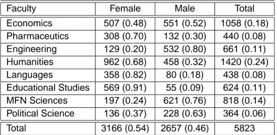
). Even though it seems strange that MFN Sciences is chosen by the individuals who attended Technical high schools, a possible explana-tion is related to the nature of the Faculty. In fact, this Faculty has several study programmes, including also informatics, subject studied in technical high schools.The distribution of final grades for high school graduates is displayed in Table (3.5). In each Faculty the percentage of students who completed their high school study with the maximum mark is quite low, except the case of Engineering students whose percentage of top students is highest (25
%
). Moreover, most high school students graduate with low grades, i.e. between60 and 79.
Faculty Licei Technical Others
Economics 354 (0.335) 699 (0.662) 3 (0.003) Pharmaceutics 307 (0.698) 106 (0.241) 27 (0.061) Engineering 377 (0.573) 280 (0.426) 1 (0.001) Humanities 948 (0.668) 374 (0.262) 100 (0.070) Languages 274 (0.634) 151 (0.350) 7 (0.016) Educational Studies 404 (0.647) 148 (0.237) 72 (0.116) MFN Sciences 315 (0.386) 489 (0.598) 13 (0.016) Political Science 149 (0.413) 200 (0.554) 12 (0.033) Total 3128 (0.54) 2444 (0.42) 235 (0.04)
Table 3.4: Distribution of students, for Faculty and High School. (Percentage
values are given in parentheses.)
Faculty 60-69 70-79 80-89 90-99 100 Economics 269 (0.26) 241 (0.23) 227 (0.22) 169 (0.16) 150 (0.14) Pharmaceutics 100 (0.23) 115 (0.26) 79 (0.18) 67 (0.15) 77 (0.18) Engineering 116 (0.18) 130 (0.20) 117 (0.18) 134 (0.20) 161 (0.25) Humanities 402 (0.28) 339 (0.24) 320 (0.23) 207 (0.15) 150 (0.11) Languages 89 (0.21) 97 (0.23) 114 (0.27) 83 (0.19) 46 (0.11) Educational Studies 222 (0.36) 195 (0.31) 129 (0.21) 52 (0.08) 26 (0.04) MFN Sciences 252 (0.31) 215 (0.26) 151 (0.18) 113 (0.14) 86 (0.11) Political Science 135 (0.37) 106 (0.29) 62 (0.17) 38 (0.11) 20 (0.06) Total 1585 (0.27) 1438 (0.25) 1199 (0.21) 863 (0.15) 716 (0.12)
Table 3.5: Distribution of students, for Faculty and high school final grades.
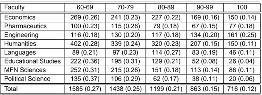
Some information on the dropout rate are reported in Tables (3.6)-(3.7). Students with a higher probability of dropping out, are those who enrolled at Political Science (59
%
) and Educational Studies (57%
), whereas Engi-neering students have the highest rate of graduation. In fact, only 33%
of students in Engineering leave the Faculty without completing the course of study. Moreover, male undergraduate in Political Science and female stu-dents in Educational Studies have the highest rates of leaving the Univer-sity.Looking at Table (3.8), it can be noted how the number of people en-rolled at the University decreased over time, and at the end of the first year, about 26
%
of students leave the University, percentage that decrease across the years. This means that pretty high number of students decide not to continue the study during the first year.Faculty No Dropout Dropout
Economics 601 (0.57) 457 (0.43) Pharmaceutics 278 (0.63) 162 (0.37) Engineering 444 (0.67) 217 (0.33) Humanities 771 (0.54) 649 (0.46) Languages 278 (0.63) 160 (0.37) Educational Studies 270 (0.43) 354 (0.57) MFN Sciences 473 (0.58) 345 (0.42) Political Science 149 (0.41) 215 (0.59) Total 3264 (0.56) 2559 (0.44)
Table 3.6: Completing and dropping out rates for Faculty. (Percentage
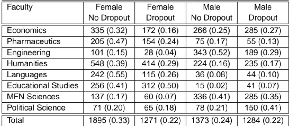
Faculty Female Female Male Male No Dropout Dropout No Dropout Dropout Economics 335 (0.32) 172 (0.16) 266 (0.25) 285 (0.27) Pharmaceutics 205 (0.47) 154 (0.24) 75 (0.17) 55 (0.13) Engineering 101 (0.15) 28 (0.04) 343 (0.52) 189 (0.29) Humanities 548 (0.39) 414 (0.29) 224 (0.16) 235 (0.17) Languages 242 (0.55) 115 (0.26) 36 (0.08) 44 (0.10) Educational Studies 256 (0.41) 312 (0.50) 15 (0.02) 41 (0.07) MFN Sciences 137 (0.17) 60 (0.07) 336 (0.41) 285 (0.35) Political Science 71 (0.20) 65 (0.18) 78 (0.21) 150 (0.41) Total 1895 (0.33) 1271 (0.22) 1373 (0.24) 1284 (0.22)
Table 3.7: Distribution of male and female, who complete or leave the
uni-versity, for Faculty. (Percentage values are given in parentheses.)
Year Number of students Year Number of Dropouts
2002 5823
2003 4297 At the end of First Year 1526 (0.26) 2004 3696 At the end of Second Year 601 (0.14) 2005 3433 At the end of Third Year 262 (0.071) 2006 3264 At the end of Fourth Year 169 (0.049)
Table 3.8: Number of students enrolled and the Number of Dropouts across
4 Statistical framework of Survival Analysis
In dropout studies, data collection must end at some arbitrarily-defined period without some of subjects having experienced the event of taking the degree. In other words, a student, at the end of the study programme may either receive the degree or leave the university. Thus, there are two differ-ent time points: the time of origin, i.e. the time at which an original evdiffer-ent, such as enrolment at the university, occurs, and the time of failure, i.e. the time at which the final event, such as dropping out at the university, takes place. In this ways, it is dealt with censored observations, i.e. observations with incomplete information about event of interest.
To study the relationship between the occurrence of events and selected predictors, Survival Analysis techniques, which incorporate both censored and uncensored observations, have been used. Moreover, it is possible to study time-varying predictors, those whose values change from one year to the next during the observation period, and to allow the effects of these variables to vary over time, modeling dynamic processes.
One of the aim of survival analysis is to estimate the survival probability function by Kaplan-Meier (KM) estimator (1958), which is usually derived as a non-parametric maximum likelihood estimate of the survivor function.
Assume that
T
i(i = 1, . . . , n) is an arbitrary non-negative random vari-able, corresponding to duration of studies of theith
individual, having a cumulative distribution function given by:F (t) = P (T ≤ t) =
Z
t0
f (u)du,
(4.1)where
f (u)
is the probability density function.Assume that the
T
i (i = 1, . . . , n) are i.i.d. with survivor functionS(t),
that is the probability of an individual surviving beyond timet, given by:
S(t) = P (T ≥ t) = 1 − F (t) =
Z
∞t
f (u)du
(4.2)It is a monotone decreasing continuous function with
S(0) = 1
andS(∞) = lim
t→∞S(t) = 0.
The
T
i (i = 1, . . . , n) are also characterized by failure rate given bycumulative hazard function
Λ(t)
, to be estimated, and it is given by:Λ(t) =
Z
t 0λ(u)du = log(S(t))
(4.3) so that:S(t) = exp[−Λ(t)] = exp[−
Z
t 0λ(u)du]
(4.4)where
λ(u)
is the Hazard function is the probability that an individual dies at timet, i.e. dropping out, conditional on having survived to that time, and
it is given by:λ(t) = −
f (t)
S(t)
(4.5)Let
C
i (i = 1, . . . , n) be the censoring time, i.e. the time between the time of enrolment and the moment of dropping out of the University for theith individual, and let
Z
i= min(T
i, C
i),
(4.6)and
δ
i= I[T
i≤ C
i],
(4.7)where
δ
iis an indicator function, equal to 1 if the student does not complete his study, and zero, otherwise.Assume that
(Z
i, δ
i)
is observed.An important assumption of the Kaplan-Meier method is that the prob-ability of a censored observation is independent of the actual survival time. In other words, the reason for which one individual is censored, is unrelated to the reason of dropping out, and the individuals whose survival times are censored, are a sample having the same distribution.
Assuming that
T
i andC
i (i = 1, . . . , n) are independent, consider the indicator function that the individuali
is still under observation at timet, i.e.
the individuali
is still enrolled at the university at timet:
where
I[.]
is an indicator function. LetN
i(t) = I[T
i≤ t, δ
i= 1]
(4.9)be the number of observed failures for individual
i, i.e. the number of
ob-served students who leave the university, whereδ
i= I[T
i≤ C
i]
.Let:
¯
Y (t) =
nX
iY
i(t) =
nX
iI[Y
i≥ t]
(4.10)be the number of subjects at risk for failure at time
t, i.e. the number of
students who are at risk for dropping out, and let:¯
N (t) =
nX
iN
i(t) =
nX
iI[N
i≤ t, δ
i= 1]
(4.11) be the total number of individual failures up to and includingt, i.e. the total
number of dropouts up to and includingt.
Consider a partition of the interval
[0, t]
, such that0 = t
1< t
2< · · · <
t
m= t
; and assume thatN
¯
kis the number of dropouts in[t
k−1, t
k]
, andY
¯
k is the number of students at risk at timet
0k, so that for small∆t
:Λ(t + ∆t) − Λ(t) ≈ λ(t)∆t
≈ P [t ≤ T < t + ∆t|T ≥ t].
(4.12) This might be estimated by [ ¯N (t+∆t)− ¯Y (t)¯ N (t)].If the sum of these quantities over subintervals
[0, t
k)
is considered and if the subintervals get small enough that they contain at most one event times, an estimator ofΛ(t)
is:b
Λ(t) =
Z
t 0d ¯
N (s)
¯
Y (s)
(4.13)called Nelson-Aalen estimator.
estimator of survival curve is obtained:
b
S(t) = exp[−b
Λ(t)] =
Y
k:ti≤texp
·
−
∆N (t
¯
i)
Y (t
i)
¸
≈
Y
k:ti≤texp
·
1 −
∆N (t
¯
i)
Y (t
i)
¸
(4.14)that is the Kaplan-Meier estimator, where
∆ ¯
N (t) = ¯
N (t) − ¯
N (t−).
The asymptotic variance of Kaplan-Meier estimator is equal to:σ
2(t) = S
2(t)
Z
t0
dF (s)
[1 − F (s)]
2− (1 − G(s))
(4.15)where
G(t) = P [C
i≤ t], and it is estimated by:
ˆ
σ
2(t) = ˆ
S
2(t)
Z
t 0nd ¯
N (s)
( ¯
Y (s))
2 (4.16)For more details, see Fleming and Harrigton (1991).
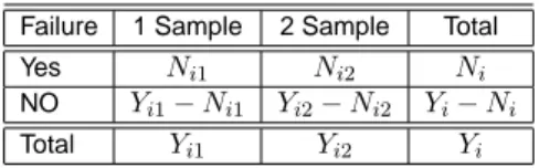
Another aim of Survival Analysis is to compare the survival curves of two or more groups, that usually is made by the Log-rank test (Mantel, 1966; Cox, 1972; Peto and Peto, 1972). It is used to test the null hypothesis that there is no difference between the population survival curves (i.e. the proba-bility of an event occurring at any time point is the same for each population). This test does not allow more than one explanatory variable to be taken into account and gives equal weight to early and late failures.
Assume
t
01≤, . . . , ≤ t
0Lare the ordered observed distinct failure times, i.e. duration of the studies, in the sample formed by combining two groups. LetN
ij andY
ij(i = 1, . . . , n; j = 1, 2) be the number of observed failures, i.e. the number of the observed dropouts and the number at risk, i.e. the number of students who are at risk of non-completing the study, in samplej
at timet
0i, respectively. LetN
iandY
ibe the corresponding values in the combined groups. The data att
0i are summarized in Table (4.1):Given
Y
ij, theN
ij have a binomial distribution with number of trialY
ij and, under the hypothesis of a common failure rateλ
in the two groups,Failure 1 Sample 2 Sample Total
Yes Ni1 Ni2 Ni
NO Yi1− Ni1 Yi2− Ni2 Yi− Ni Total Yi1 Yi2 Yi
Table 4.1: Number of cases failing and not failing at
t
0i from those at risk, by sampleapproximate event probability
λ(t
0i)∆t
. Fisher’s exact test for equal binomial parameters in this setting is based on conditioning further onYi
and on using the resulting conditional hypergeometric distribution forYi1. This distribution
will have conditional mean²i1
and varianceυi1
given by:²i1
= N
iYi1
Yi
(4.17) andυi1
= N
iYi1Yi2
Y
2 iYi
− Ni
Yi
− 1
(4.18)Considering the vector of observed death times minus conditionally ex-pected number of failures across observed failure times, and if the assumpp-tion is that these differences are independent, the statistic is:
Q =
LX
i=1
(N
i1− ²i1
).
(4.19)It can be shown that under
H
0, it is approximately a standard normal distribution:Q ≈ N (0, V ),
(4.20)where
V =
P
Li=1v
i1. So underH
0:T =
Q
2
V
≈ χ
2
If two or more survival curves are significantly different, it is possible to assess the factors that may play a role in survival probability. The Cox
Proportional Hazards (PH) Model (Cox, 1972) is useful to identify the risk
factors and their risk contributions, selecting efficiently a subset of signifi-cant variables, upon which the hazard function depends. In other words, it explores the association of covariates with failure times and survival distri-butions, and it studies the effect of a primary covariate, while adjusting for other variables.
A key characteristic of the Cox model is that the hazard ratio does not depend on time, so that it is nonparametric with respect to time, but para-metric with respect to covariates. Any distributional assumption about the baseline hazard is not made, assuming that it is common among all individ-uals.
Consider
(Z
i, δ
i, x
i)
(i = 1, . . . , n), whereZ
i is given by (4.6);δ
i is given by (4.7), andx
iare the covariates, i.e. Gender, Age at Matriculation, Type and Mark of High School, Familiar Income, Mark of Exams.Assume that covariates do not vary with time, and that
S(t|x)
is the con-ditional survival functionP (T > t|x). Thus the conditional hazard function
is given byλ(t|x) =
lim
∆t→∞
1
∆t
P [t ≤ T ≤ t + ∆t|T ≥ t, x]
(4.22)If T is the failure time variable i.e. duration of studies, a partition on T is defined so that
0 = t
0≤ t
1≤ · · · ≤ t
m< ∞, and consider a new variable
T
∗= t
iift
i≤ T < t
i+1(i = 0, 1, . . .).In this case, the conditional hazard function on the discrete distribution of
T
∗is given by:λ
∗(t
i|x) = P [T
∗= t
i|T
∗≥ t
i, x]
i = 0, 1, . . .
(4.23) and in terms of original distribution ofT
:λ
∗(t
i|x) = 1 − exp
·
−
Z
ti+1 tiλ(u|x)dx
¸
(4.24) Assuming that a model with arbitrary covariatex
has, for eacht
i, con-ditional odds of failing in an interval[t
i, t
i+1]
proportional to the model withcovariate
x = 0, then for each
t
iλ
∗(t
i|x)
1 − λ
∗(t
i|x)
=
λ
∗ 0(t
i)
1 − λ
∗ 0(t
i)
g(x)
(4.25)for some function
g, where
λ
∗0(t
i) = λ
∗(t
i|x = 0).
Now, if the proportionality does not depend on the partition chosen, then it results that:
1 − exp
·
−
R
tt+∆tλ(u|x)du
¸
exp
·
−
R
tt+∆tλ(u|x)du
¸
=
1 − exp
·
−
R
tt+∆tλ
0(u)du
¸
exp
·
−
R
tt+∆tλ
0(u)du
¸
· g(x).
(4.26)In order to ensure that
q ≤ 0,
g(x) = exp(βx)
is considered. If∆ → 0
, it results:λ(t|x) = λ
0(t) · exp(β
0x)
(4.27)where
λ
o(t)
is the Baseline hazard rate,β
is the regression parameter vec-tor, estimated by maximizing a partial likelihood, without regard to the base-line hazardλ
0(t)
.Inference procedures for the PH model and the multiplicative intensity model requires computation methods for finding estimates of the regres-sion coefficients and the baseline hazard function, and at least approximate sapling distributions of those estimators.
Assume that the covariates do not vary with time, the failure distribution is continuous and there are no ties among the observed failure times.
Consider again the independent triples
(Z
i, δ
i, x
i)
,i = 1, . . . , n.
Z
ihas a density in our caseθ
isβ
andφ
isλ
0(t)
. We want to make inference onθ,
with
φ
a nuisance parameter.Z
iare transformed into(V
1, W
1, . . . , V
N, W
N)
. Suppose to observeL
failures at times0 = t
00< t
01< · · · < t
0L<
t
0L+1= ∞
. The covariates associated withL
failures areX
1, . . . , X
L. Now suppose thatn
i items are censored at or aftert
0i but beforet
0i+1, at timest
0i1, . . . , t
0i+mi. The covariates associated with them
icensored items are(X
(i,1), . . . , X
(i,mi))
. Consider a condition on{X
i: i = 1, . . . , n}
.For
i = 0, . . . , L, it results:
V
i+1= {t
0i+1, t
0ij, (i, j) : j + 1, . . . , m
i}
andW
i+1= {(i + 1)}
. In the nested sequence(P
i, Q
i)
,P
icontains the timesof all censoring up to time
t
0i−1 and the times of all failures through timest
0i−1. Instead,Q
i specifiest
0i and the times of all censoring at or aftert
0i−1 and up tot
0i.Inference for
β
could be based on the information inP
i+1givenQ
i, that is, on the partial likelihood:L
Y
i=1
P [W
i= (i)|Q
i]
(4.28)To obtain an expression for
P [W
i= (i)|Q
i]
, it is considered that the assumption of independent censoring implies that the probabilities that the item with label (i) fails att
0i= t
i, given the risk setR
i≡ {j : X
j≤ t
0i}
and given that one failure occurs att
i, is:P [W
i= (i)|Q
i] =
=
dΛ(t
i|x
(i))
Q
j6∈Ri−(i){1 − dΛ(t
i|x
j)}
P
l∈Ri£
dΛ(t
i|x
l)
Q
j∈Ri−l{1 − dΛ(t
i|x
j)}
¤
=
P
λ(t
i|x
(i))
l∈Riλ(t
i|x
l)
=
exp(β
0x
(i))
P
l∈Riλ(t
i|x
l)
(4.29) Thus, using (4.28), the partial likelihood is given by:L(β) =
LY
i=1exp(β
0x
(i))
P
l∈Riexp(β
0x
l)
(4.30)The log Partial likelihood is given by:
log L(β) =
LX
i=1½
β
0x
i− log
X
j∈Rkexp(β
0x
(j))
¾
(4.31)The efficient score for
U (β) =
∂ log L(β)∂β is:U (β) =
LX
k=1½
x
k−
P
j∈Rkx
jexp(β
0x
j)
P
j∈Rkexp(β0xj)¾
(4.32)Maximum partial likelihood estimates
β
are found using thep
simulta-neous equationsU (β) = 0, where
p
is the number of covariates.In order to make inferences on
β
based on Partial Likelihood, the func-tional form forλ
0(t)
does not be specified . It can be proved that:ˆ
β ∼ N (β, I(β)
−1)
(4.33)where
I(β)
−1is the Information matrix, and can be derived using the stan-dard methods.5 Analysis of the dropout rates at the University of Salerno
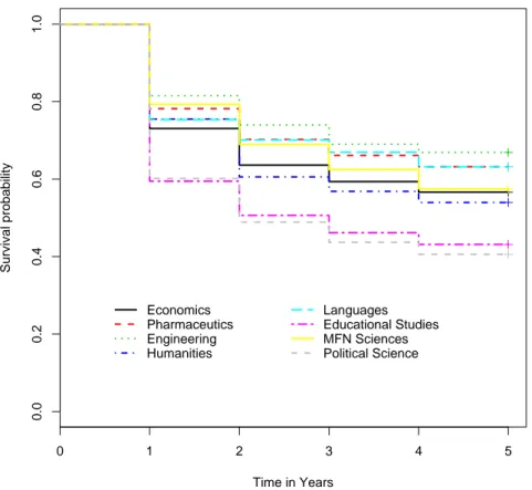
In this section, survival analysis techniques are used to estimate the dropout probability. First of all, the survival function is estimated by the Kaplan-Meier estimator. In Figure (5.1), eight different lines indicate the sur-vivor probabilities for the students who studied in one of the Faculties of the University of Salerno. It can be noted how the dynamics of departure differs by the Faculty. A steep decline is observed for the students in Political Sci-ence and in Educational Studies, at the first year. The lower survival rate for these two Faculties continue throughout the observation period. Moreover, at the end of the second year, the survival probability also decrease for the Humanities. This means that the decision of leaving the university is taken by the students enrolled at the Humanities during the second year, and not during the first year, as for students in the Political Science and Educational Studies.
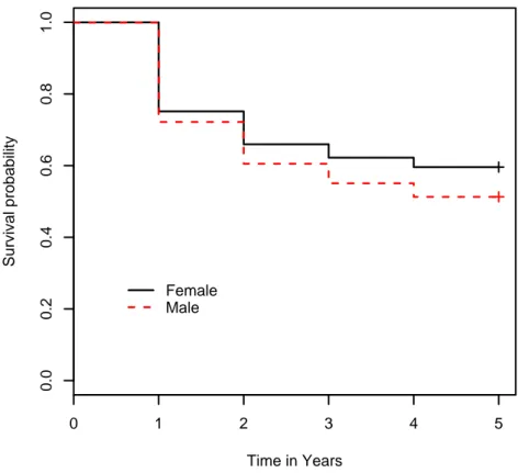
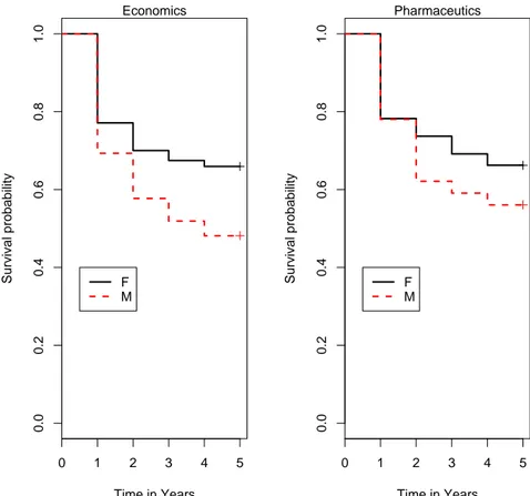
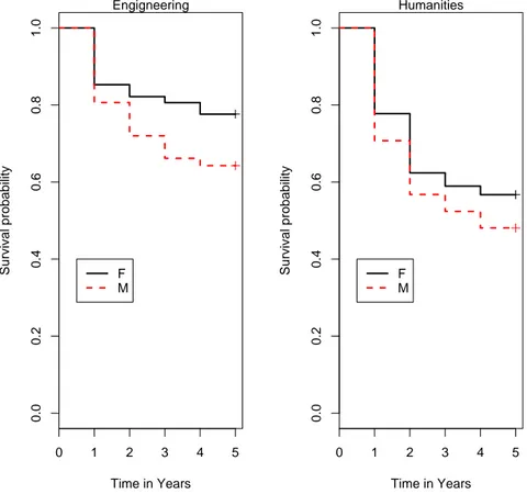
The KM estimator for males and females is shown in Figure (5.2). It can be noted how male students have lower survival rates than female. This means that males do not complete their study, and therefore leave the Uni-versity faster than females. This is true also if you look at survival func-tions of male and female, distinguishing by Faculty (Figures (5.3)-(5.6)). It is confirmed that the students in Political Science and in Educational Studies, in particular males, have lower survival rate than those in other Faculties. Moreover, the rate of dropping out for male undergraduates in Pharmaceu-tics and MFN Sciences is particularly evident at the end of the second year, while male students in Languages, Educational Studies and Political Sci-ence leave the university during the first year. Therefore, Faculty attended has an effect on probability of surviving at University.
0 1 2 3 4 5 0.0 0.2 0.4 0.6 0.8 1.0 Time in Years Survival probability Economics Pharmaceutics Engineering Humanities Languages Educational Studies MFN Sciences Political Science
0 1 2 3 4 5 0.0 0.2 0.4 0.6 0.8 1.0 Time in Years Survival probability Female Male
Figure 5.2: Survival functions for males and females, for data considered
0 1 2 3 4 5 0.0 0.2 0.4 0.6 0.8 1.0 Time in Years Survival probability Economics F M 0 1 2 3 4 5 0.0 0.2 0.4 0.6 0.8 1.0 Time in Years Survival probability Pharmaceutics F M
Figure 5.3: Survival functions for male and female, by Faculty (Economics,
0 1 2 3 4 5 0.0 0.2 0.4 0.6 0.8 1.0 Time in Years Survival probability Engigneering F M 0 1 2 3 4 5 0.0 0.2 0.4 0.6 0.8 1.0 Time in Years Survival probability Humanities F M
Figure 5.4: Survival functions for male and female, by Faculty (Engineering,
0 1 2 3 4 5 0.0 0.2 0.4 0.6 0.8 1.0 Time in Years Survival probability Languages F M 0 1 2 3 4 5 0.0 0.2 0.4 0.6 0.8 1.0 Time in Years Survival probability Educational Studies F M
Figure 5.5: Survival functions for male and female, by Faculty (Languages,
0 1 2 3 4 5 0.0 0.2 0.4 0.6 0.8 1.0 Time in Years Survival probability MFN Sciences F M 0 1 2 3 4 5 0.0 0.2 0.4 0.6 0.8 1.0 Time in Years Survival probability Political Science F M
Figure 5.6: Survival functions for male and female, by Faculty (MFN
In Figures (5.7)-(5.10), the four lines correspond to the different groups of students according to the age at the time of enrolment at the University. It can be noted how the students who are more than 24 years old, have a sur-vival rate that is lower than those who are 19 years old. Therefore, students who enrol at the University immediately after completing their high school study, have a greater probability of taking the degree than those who decide to study at the University after having completed the high school study by many years. Moreover, it can be noted that there is also a Faculty effect. This means that the probability of surviving after the first year, for older stu-dents in Economics and Engineering is lower than that for older stustu-dents in other Faculties.
The students who attend the "Licei" have the higher probability of sur-viving at the University, i.e. the higher rate of taking the degree. This results depends on the nature of the high school. Technical high schools provide a specialised qualification, so that students may find a job, also without taking the degree, whereas those who studied at the "Licei" have to continue their study, enrolling at the University, since the "Licei" provide a general qualifi-cation (Figures (5.11)-(5.14)). Also in this case, a Faculty effect is noted.
Finally, students who complete their high school study with the maxi-mum mark (i.e. 110), have the higher probability of completing their study, whereas those who have lower marks, between 60 and 79, have the lower probability of surviving, i.e. the lower rate of taking the degree and therefore the higher chance of leaving the University (Figures (5.15)-(5.18)). More-over, it can be noted how the probability of dropping out of the university for students with lower marks changes by Faculty attendend.
0 1 2 3 4 5 0.0 0.2 0.4 0.6 0.8 1.0 Time in Years Survival probability Economics 18−19 20−21 22−23 >24 0 1 2 3 4 5 0.0 0.2 0.4 0.6 0.8 1.0 Time in Years Survival probability Pharmaceutics 18−19 20−21 22−23 >24
Figure 5.7: Survival functions for students in Economics and
0 1 2 3 4 5 0.0 0.2 0.4 0.6 0.8 1.0 Time in Years Survival probability Engigneering 18−19 20−21 22−23 >24 0 1 2 3 4 5 0.0 0.2 0.4 0.6 0.8 1.0 Time in Years Survival probability Humanities 18−19 20−21 22−23 >24
Figure 5.8: Survival functions for students in Engineering and Humanities,
0 1 2 3 4 5 0.0 0.2 0.4 0.6 0.8 1.0 Time in Years Survival probability Languages 18−19 20−21 22−23 >24 0 1 2 3 4 5 0.0 0.2 0.4 0.6 0.8 1.0 Time in Years Survival probability Educational Studies 18−19 20−21 22−23 >24
Figure 5.9: Survival functions for students in Languages and Educational
0 1 2 3 4 5 0.0 0.2 0.4 0.6 0.8 1.0 Time in Years Survival probability MFN Sciences 18−19 20−21 22−23 >24 0 1 2 3 4 5 0.0 0.2 0.4 0.6 0.8 1.0 Time in Years Survival probability Political Science 18−19 20−21 22−23 >24
Figure 5.10: Survival functions for students in MFN Sciences and Political
0 1 2 3 4 5 0.0 0.2 0.4 0.6 0.8 1.0 Time in Years Survival probability Economics Licei Tech−Prof Others 0 1 2 3 4 5 0.0 0.2 0.4 0.6 0.8 1.0 Time in Years Survival probability Pharmaceutics Licei Tech−Prof Others
Figure 5.11: Survival functions of students in Economics and
0 1 2 3 4 5 0.0 0.2 0.4 0.6 0.8 1.0 Time in Years Survival probability Engigneering Licei Tech−Prof Others 0 1 2 3 4 5 0.0 0.2 0.4 0.6 0.8 1.0 Time in Years Survival probability Humanities Licei Tech−Prof Others
Figure 5.12: Survival functions of students in Engineering and Humanities,
0 1 2 3 4 5 0.0 0.2 0.4 0.6 0.8 1.0 Time in Years Survival probability Languages Licei Tech−Prof Others 0 1 2 3 4 5 0.0 0.2 0.4 0.6 0.8 1.0 Time in Years Survival probability Educational Studies Licei Tech−Prof Others
Figure 5.13: Survival functions of students in Languages and Educational
0 1 2 3 4 5 0.0 0.2 0.4 0.6 0.8 1.0 Time in Years Survival probability MFN Sciences Licei Tech−Prof Others 0 1 2 3 4 5 0.0 0.2 0.4 0.6 0.8 1.0 Time in Years Survival probability Political Science Licei Tech−Prof Others
Figure 5.14: Survival functions of students in MFN Sciences and Political
0 1 2 3 4 5 0.0 0.2 0.4 0.6 0.8 1.0 Time in Years Survival probability Economics 60−69 70−79 80−89 90−99 100 0 1 2 3 4 5 0.0 0.2 0.4 0.6 0.8 1.0 Time in Years Survival probability Pharmaceutics 60−69 70−79 80−89 90−99 100
Figure 5.15: Survival functions of students in Economics and
0 1 2 3 4 5 0.0 0.2 0.4 0.6 0.8 1.0 Time in Years Survival probability Engigneering 60−69 70−79 80−89 90−99 100 0 1 2 3 4 5 0.0 0.2 0.4 0.6 0.8 1.0 Time in Years Survival probability Humanities 60−69 70−79 80−89 90−99 100
Figure 5.16: Survival functions of students in Engineering and Humanities,
0 1 2 3 4 5 0.0 0.2 0.4 0.6 0.8 1.0 Time in Years Survival probability Languages 60−69 70−79 80−89 90−99 100 0 1 2 3 4 5 0.0 0.2 0.4 0.6 0.8 1.0 Time in Years Survival probability Educational Studies 60−69 70−79 80−89 90−99 100
Figure 5.17: Survival functions of students in Languages and Educational
0 1 2 3 4 5 0.0 0.2 0.4 0.6 0.8 1.0 Time in Years Survival probability MFN Sciences 60−69 70−79 80−89 90−99 100 0 1 2 3 4 5 0.0 0.2 0.4 0.6 0.8 1.0 Time in Years Survival probability Political Science 60−69 70−79 80−89 90−99 100
Figure 5.18: Survival functions of students in MFN Sciences and Political
To be sure that there is a significant difference among the survival curves, as emerged in the previous Figures, the equality of the survivor functions is tested by the Log-rank test, where the null hypothesis is that the sur-vival curves are equal. The Table (5.1) shows the values of p-value for each log-rank tests, by to Gender, Age at the time of the enrolment, Type of High School, and the high school final grades. It can be noted how the null hypothesis is always rejected, choosing a significance level equal to 0.05. Thus, it is confirmed that there is a significant difference in survival curves, between Males and Females, according to the Age of student at the moment of entry at the Univeristy, the Type of High School attended by the students, and the final mark received at the high school.
Faculty Gender Age High School High School Mark
Economics <0.001 0 <0.001 0 Pharmaceutics 0.048 <0.001 <0.001 <0.001 Engineering 0.004 0 <0.001 <0.001 Humanities 0.002 0 <0.001 <0.001 Languages <0.001 <0.001 <0.001 <0.001 Educational Science <0.001 <0.001 <0.001 <0.001 MFN Sciences <0.001 0 <0.001 0 Political Science <0.001 <0.001 <0.001 <0.001 Total <0.001 0 0 0
Table 5.1: P-values of Log-rank tests for testing the difference in survival
curves according to some covariates.
A limitation of using the log-rank test is that it does not allow more than one explanatory variable to be taken into account. In fact, it may be interest-ing to analyse the interrelations between the covariates, and explored the influence of covariates on failure times. Studying the effect of a primary co-variate, while adjusting for other variables, allow to select efficiently a subset of significant variables, upon which the hazard function depends. For this purpose, a Cox Proportional Hazards model is used.
to test two nested models.
The most significant variables for the Cox PH model, for each Faculty and when the data are anlysed entirely are shown in Table (5.2)-(5.10). A positive estimated coefficient indicates an increased hazard and hence a shorter expected survival time. Consequently, a negative estimated coef-ficient denotes a decreased hazard, and therefore a greater expected sur-vival time. It is confirmed that there is a significant difference of the sursur-vival curves among Faculties, between males and Females, according to the Age at the time of the enrolment, the type and mark of high school, according to the family level income and the average mark of exams taken at the Univer-sity.
The difference between males and females is validated for Pharmaceu-tics, Engineering, Humanities, MFN Sciences, and Political Science. In par-ticular the estimated coefficient is positive and it means that male students have an increased hazard and therefore a shorter expected survival time than females. In other words, males students may leave the university more quickly than females.
The age at the moment of the enrolment is significant for all faculties, and it has a positive coefficients. Therefore, the probability that the older students do not complete their study is higher than that of female group. Looking at the high school final grades and the mark of exams, it can be noted how the student with higher marks, have a decreased hazard and hence a longer expected survival time than those with lower marks. Thus, their chance to take the degree is higher than that of other group.
Fixing the other covariates, the hazard ratio between males and females is equal to 1.37. This means that, with other covariates fixed, males students are 1.37 time more likely than females students to have shorter survival rate. Now a male student in Political Science is 1.33 time more likely than a male student in Economics to have shorter survival rate. Then a older male stu-dent is 5.90 time more likely than a youger male stustu-dent to have shorter survival rate.
coef se(coef) se2 Chisq p Facolty 0.0412 1.042 0.0117 3.52 <0.001 Gender 0.3170 1.373 0.1287 2.46 0.014 Age 0.5915 1.807 0.0976 6.06 <0.001 High School Mark -0.2048 0.815 0.0270 -7.58 <0.001 Income 0.0971 1.102 0.0163 5.97 <0.001 Mark of Exams -0.2168 0.805 0.0329 -6.60 <0.001 High School -0.0547 0.947 0.0144 -3.79 <0.001 Gender:Age -0.1475 0.863 0.0612 -2.41 0.016
Table 5.2: Cox Proportional Hazards Model, considering the data entirely.
coef se(coef) se2 Chisq p Age 0.509 1.66 0.0807 6.31 <0.001 High School Mark -0.174 0.84 0.0718 -2.42 0.015 Income 0.132 1.14 0.0405 3.26 <0.001 Mark of Exams -0.635 0.53 0.1259 -5.05 <0.001
coef se(coef) se2 Chisq p Gender 1.477 4.378 0.5381 2.74 <0.001 Age 1.572 4.818 0.3746 4.20 <0.001 High School Mark -0.299 0.742 0.1044 -2.86 <0.001 Income 0.105 1.110 0.0607 1.72 0.081 Mark of Exams -0.286 0.751 0.1332 -2.15 0.032 Gender:Age -0.889 0.411 0.2851 -3.12 <0.001
Table 5.4: Cox Proportional Hazards Model, for Pharmaceutics.
coef se(coef) se2 Chisq p Gender 0.7711 2.162 0.5460 1.41 0.016 Age 1.8336 6.257 0.5627 3.26 <0.001 Income 0.0918 1.096 0.0462 1.99 0.047 Mark of Exams -0.9499 0.387 0.1257 -7.55 <0.001 Gender:Age -0.6414 0.527 0.2993 -2.14 0.032
Table 5.5: Cox Proportional Hazards Model, for Engineering.
coef se(coef) se2 Chisq p Gender 0.3108 1.365 0.1420 2.19 0.029 Age 0.3604 1.434 0.0705 5.11 <0.001 High School Mark -0.1677 0.846 0.0594 -2.82 <0.001 Income 0.0791 1.082 0.0352 2.25 0.025 Mark of Exams -0.1704 0.843 0.0686 -2.49 0.013
Table 5.6: Cox Proportional Hazards Model, for Humanities.
coef se(coef) se2 Chisq p Age 0.315 1.370 0.1469 2.144 0.032 High School Mark 0.025 1.025 0.1117 0.224 0.042 Income 0.207 1.230 0.0609 3.402 <0.001 Mark of Exams -0.935 0.393 0.1666 -5.612 <0.001
coef se(coef) se2 Chisq p Age 0.308 1.360 0.0824 3.73 <0.001 Income 0.108 1.114 0.0486 2.23 0.026 Mark of Exams -0.486 0.615 0.1092 -4.45 <0.001
Table 5.8: Cox Proportional Hazards Model, for Educational Studies.
coef se(coef) se2 Chisq p
Gender -0.9720 0.378 0.6601 -1.47 0.042
Age 0.3412 1.407 0.0826 4.13 <0.001
Mark of High school 0.4170 1.517 0.2944 1.42 0.016
Income 0.0734 1.076 0.0404 1.82 0.029
Mark of Exams -1.9933 0.136 0.4883 -4.08 <0.001 High School -0.1030 0.902 0.0344 -3.00 <0.001 Gender:High School Mark -0.3966 0.673 0.1617 -2.45 0.014 Gender:Mark of Exams 0.9510 2.588 0.2602 3.66 <0.001
Table 5.9: Cox Proportional Hazards Model, for MFN Sciences.
coef se(coef) se2 Chisq p Gender 1.057 2.878 0.5075 2.08 0.0370 Age 0.961 2.615 0.3219 2.99 0.0028 Income 0.135 1.144 0.0592 2.28 0.0230 Mark of Exams -0.454 0.635 0.1469 -3.09 0.0020 Gender:Age -0.426 0.653 0.1931 -2.21 0.0270
Two important issues in Cox PH model are related to testing the propor-tional hazard assumption, i.e. if the proporpropor-tional hazard assumption holds on, and to verifying the influence of some observations on estimating the model. The p-values of test for verifying the existence of the proportional hazard assumption are shown in Table (5.11)-(5.13). It can be noted how in some models, mark of exams and family income level seems to be not pro-portional. In other words, for these two covariates, the proportional hypoth-esis does not hold on. This might depend on the presence of linear trend in the hazards. In other words, some covariates could be time-varying, and it is important to check if they change over time. In these models, this control cannot be made, since the factors are not continuous.
Full Data Economics Pharmaceutics
Faculty 0.48
Gender 0.15 0.20
Age 0.07 0.18 0.21
High School Mark 0.65 0.45 0.64
Income <0.05 <0.05 0.96
Mark of Exams <0.05 <0.05
High School 0.23
Gender:Age 0.05 0.30
Table 5.11: P-values of the test on proportional hazard assumption, for
model with all data, for Economics, Pharmaceutics.
Another issue in Cox PH model is related to the influence of single ob-servation on estimating the models. Therefore if a particular subject affects the estimated coefficients, it would be eliminated from the data, and the model should be estimated again. To evaluate the influence of individuals on the estimated
β
coefficients, the dfbetas values are used. In particu-lar, dfbetas is approximately the change in the coefficients scaled by their standard error. Comparing the magnitudes of the largest dfbeta values to the estimated coefficients, there are no subject’s influence on the estimated coefficient.Engineering Humanities Languages
Gender 0.58 0.62
Age 0.93 0.16 0.14
High School Mark 0.43 0.81
Income 0.71 <0.01 0.08
Mark of Exams 0.31 0.06 <0.05
High School
Gender:Age 0.66
Table 5.12: P-values of the test on proportional hazard assumption, for
En-gineering, Humanities, Languages.
Educational Studies MFN Sciences Political Science
Gender 0.92 0.46
Age 0.21 0.13 0.57
High School Mark 0.37
Income 0.59 0.11 0.99
Mark of Exams 0.81 0.60 0.09
High School 0.44
Gender:Age 0.89
Gender:Mark of High School 0.67
Gender:Mark of Exams 0.77
Table 5.13: P-values of the test on proportional hazard assumption, for
6 Concluding remarks
The aim of this paper was to analyse and model the interval of time between the first enrolment at University and the first occurrence of non-enrolment, so that the event of interest is the dropping out of University. The data consists of the full-time students enrolled at the University of Salerno at the 2002-2003 academic year, and they are analysed by Survival Analysis models.
This study has shown that there is a steep decline for the students in Political Science and in Educational Studies, at the first year. Moreover, male students have lower survival rates than female students, i.e. they leave the University earlier than female group. Moreover, students who enrol at the University immediately after completing their high school study, have greater probability of taking the degree than those who decide to study at the University after having completed the high school study by many years. Students who attended "Licei" have the highest probability of surviving at the University, i.e. the highest rate of taking the degree. Students who complete their high school study with the highest mark (i.e. 110), have the highest probability of completing their study. In all these cases, it can be noted that there is a Faculty effect. These differences are confirmed by Log-rank test and Cox Proportional Hazards Model.
The study confirms most of the substantive findings of earlier research illustrated in Section 2, where it has been underlined how gender and age influence the probability of completing the study, how income and precollege qualification affect the decision of dropping out of the University.
References
Arulampalam W. and Naylor R.A. and Smith J.P. (2004): A hazard model of the probability of medical school drop-out in the UK, Journal of Royal
Statistical Society Series A, 167, pp. 157-178.
Arulampalam W. and Naylor R.A. and Smith J.P. (2005): Effects of in-class variation and student rank on the probability of withdrawal: cross-section and time series analysis of UK universities students, Economics of
Education Review, 24, pp. 251-262.
Astin A. (1964): Personal and environmental factors associated with college dropout among high aptitude students, Journal of Educational
Psychology, 55, pp. 219-227.
Bayer A. (1964): The college dropout: Factors affecting senior college completion, Sociology of Education, 41, pp. 305-316.
Bean J.P. (1980): Dropouts and turnover. The synthesis and test of a casual model of student attrition, Research in Higher Education, 12, 2, pp. 155-187.
Bean J.P. (1982): Student attrition, intentions, and confidence: Interactions effects in a path mdoel. Research in Higher Education, 17, 4, pp. 291-319. Bean J.P. and Metzner B.S. (1983): A conceptual model of nontraditional undergraduate student attrition, Review of Educationl Research, 55, pp. 485-540.
Bratti M., Broccolini C. and Staffolani S. (2006): Is "3+2" Equal to 4? University Reform and Student Academic Performance in Italy, DEA
Working Paper no. 251, Università Politecnica delle Marche, Ancona.
Bratti M., Broccolini C. and Staffolani S. (2007): Mass tertiary education, higher education standard and university reform: a theoretical analysis,
Working Paper no. 277, Università Politecnica delle Marche, Ancona.
Braxton J.M., Duster M. and Pascarella E.T. (1988): Casual modeling and path analysis: An introduction and an illustration in student attrition research, Journal of College Student Development, 29, 3, pp. 263-272. Cabrera A.F., Nora A. and Castaneda M.B. (1993): College persistence:
Structural equation modeling test of an integrated model of student retention, Journal of Higher Education, 64, 2, pp. 123-139.
Checchi D., Ichino A. and Rustichini A. (1999): More equal but less mobile? Education financing and intergenerational mobility in Italy and in the US,
Journal of Public Economics, 74, pp. 351-393.
Checchi D. and Flabbi L. (2006): Intergenerational Mobility and Schooling Decisions in Italy and Germany, Mimeo, University of Milan.
Cingano F. and Cipollone P. (2003): Determinants of the university dropout probability in Italy, Annual Meeting of the European Association of Labour Economists, Seville, Spain.
Collett D. (1994): Modelling survival data in medical research, Chapman and Hall.
Cox D.R. (1972): Regression models and lifetables (with discussion), J.R.
Stat Soc. B, 34, pp. 187-220.
Cox D.R. and Oakes D. (1984): Analysis of Survival Data, Chapman and Hall.
DesJardinis S.L., Ahlburg D.A. and McCall B.P. (1999): An event history model of student departure. Economics of Education Review,18, 3, pp. 375-390.
interrupted enrolment on graduation from college: Racial, income and ability differences. Economics of Education Review, 25, 6, pp. 575-590. Di Pietro G. and Cutillo A. (2006): The impact of supply side policies on
university drop-pout: The Italian experience, paper presented at the
EALE 2006 Conference (Prague).
Eckstein Z. and Wolpin K. (1999): Why youths drop out of high school the impact of preferences, opportunities and abilities, Econometrica, Vol. 67,no. 6, pp. 1295-1339.
Fleming T.R. and Harrington D.P. (1991): Counting processes and Survival
analysis, Wiley-Interscience.
Hougaard P. (2000): Analysis of multivariate survival data, Springer. Ishitani T.T: (2003): A longitudinal approach to assessing attrition behavior
among first-generation students: Time-Varying Effects of Pre-College Characteristics, Research in Higher Education, 44, 4, pp. 433-449. Johnes G. and McNabb R. (2004): Never five up on the good times: student
attrition in the UK, Oxford Bulleting of Economics and Statistics, 66, pp. 23-47.
Johnes G. (1990): Determinants of student wastage in higher education,
Studies in Higher Education, 15, pp. 87-99.
Johnson I.Y. (2006): Analysis of stopout behavior at a public research university: The Multi-Spell Discrete-Time Approach, Research in Higher
Education, 47, 8, pp. 905-934.
Kalamatianou A.G. and McClean S. (2003): The Perpetual Student: Modeling Duration of Undergraduate Studies Based on Lifetime-Type Education Data, Lifetime Data Analysis, 9, pp. 311-330.