EVOLUTION OF SURVIVAL AT OLD AGES DURING
THE 20TH CENTURY IN EMILIA ROMAGNA
R. Rettaroli, G. Roli, A. Samoggia
1. INTRODUCTION AND BACKGROUND
In the period from 18711 to 2007, Italian mortality profiles by sex and age changed substantially at both regional and sub-regional levels. The study of this evolution describes the different phases and the nature of the epidemiological transition that took place during the course of the one hundred and thirty years period under study, which was characterised by a gain in the mean duration of life of about 47 years, and a rise in life expectancy at birth from 32.7 to 80.1 years for both sexes.
The Italian mortality transition and the reduction in the mortality rates at all ages have been studied in depth by various researchers (Pozzi, 2000; Caselli, 1990, 2007): the evolution of sex and age mortality schedules, as well as the differences at the national and regional level, have been described and related to changes in the incidence of the different causes of death. The rapid, clear fall in mortality was associated with profound changes in the prevailing patterns of disease and morbidity.
Within this framework, the role of the fall in infant and youth mortality, espe-cially in the first stage of the mortality transition, is crucial and has often drawn the attention of specialists through the analysis of the trends and the main causes affecting the lower half of the age range. Although the greatest gains in life expec-tancy have been mainly due to such specific age groups since the mid-1980s, it is clear that the occurrence of death has been postponed to older ages as the risks of dying at an earlier age fell dramatically (Caselli and Capocaccia, 1989). By the 1970s, the decline in mortality rates had already been extended to all ages, while the fall in the risk of dying at an older age had not bottomed out. Besides, the changes in adult and old age mortality patterns showed some considerable geo-graphical variability, as it had been observed before for survival at earlier ages, thus justifying the specific interest in a sub-national level research approach (Caselli and Lipsi, 2006).
1 1871 practically constitutes the first date at which it is possible to calculate complete life tables at a national, regional and sub-regional level for Italy.
In this paper we focus on the explanation and description of the long trend survival and mortality in Emilia-Romagna region. We present some partial results of elderly male and female survival patterns over the last one hundred and thirty years, including a comparison with the situation in Italy as a whole.
Starting from the fact that as things stand, mortality is concentrated at older ages, we also study the evolution of modal age at death. Indeed, this indicator provides an appealing perspective from which the shifting and compression mor-tality hypotheses can be investigated (Fries, 1980; Myers and Manton, 1984; Kan-nisto, 1996; Bongaarts, 2005; Robine et al., 2008).
These initial results constitute a pivotal part of a broader research project aim-ing at exploraim-ing the mechanisms underpinnaim-ing the long-term transition in adult and elderly survival, from the first phase of the demographic transition to the present day2. A further specific aim of our work is to fill in the gap in the histori-cal long trend analysis due mainly to the different ways mortality and population data are collected.
The great amount of available information, concerning both mortality and causes of death after 1950s, often contrasts with the lack of in-depth studies re-lated to the more recent or distant past. This situation can prevent scholars from having a long-trend vision of the prevailing changes.
Emilia Romagna, a region in North-East Italy, is an appropriate choice for studying adult and elderly mortality profiles. Indeed, over the last decade it has boasted one of the oldest regional age structures in Europe (with 22.6% of peo-ple aged 65+, and 6.8% aged 80+ in 2008, from a total population of 4,275,802). Since the 1970s, the absolute numbers of elderly have been continuously increas-ing, while adult and elderly mortality rates have been falling (along different paths and at different speeds for men and women) more than anywhere else in Italy. These trends call for explanations, especially in terms of the analysis of geo-graphical variations within the region according to the structure and the preva-lence of causes of death. This aspect can also be related to the increase in popula-tion longevity and the characteristics thereof.
The paper is structured as follows. The second section introduces the reader to the data and the methods employed to estimate life tables and the main indicators of survival. The third section describes the long trend evolution of survival pat-tern in Emilia Romagna, from 1871 to 2007. The fourth section underlines the differences between men and women survival, and the different weights of age spans in the rise in life expentancy at birth. The fifth section examines the changes in the modal age at death and in the concentration of deaths around the mode. Finally, the last section offers a discussion of our findings together with our conclusions.
2 The research project team consist of a broad group of researchers (demographers, statisticians, geneticists), of the Bologna province Statistical Office and of the “Fondazione del Monte di Bolo-gna e Ravenna”, the latter of which has granted this study.
2. DATA AND METHODS 2.1. Description of raw data
The mortality and population data used in this study were taken from official statistics published by ISTAT (The Italian National Statistics Institute) and by the Statistics Department of Emilia-Romagna.
The data firstly consist of the number of deaths, by sex and age, per calendar year around the dates of the various population censuses conducted between 1871 and 20013. For the year 2007, data are provided by the Emilia Romagna region’s Statistics Department. The availability of detailed death counts changes over the course of the period in question. From 1930 on, all deaths are classified according to single year of age of the deceased; in previous years, however, only 5-year age group classifications are available. Centenarian deaths are only tabulated in detail from 1950 onwards. In 1901 they are nested into the last open age interval of 90+. Otherwise, the deaths at age 100 and over are given as a lump sum.
Furthermore, census results for the present population, by sex and age, are also considered. The age classification of the population, as published by official agen-cies, changed during the census years. In 1871 and 1931 all individuals are classi-fied by single year of age up to age 99. From 1881 to 1921, only population data classified according to 5-year age groups are available up to the last open interval, which is of 90+ in 1901 and 100+, otherwise. In 1936 and 1951, one part of the elderly ages are collapsed into 5-year age groups (from age 75 and over in 1936 and from age 80 in 1951). Finally, from 1961 on, all individuals have been classi-fied by single year of age (up to age 109 in the last two censuses and up to age 99, otherwise). In all cases, except for the 1901, 1991 and 2001 censuses, centenarians are given as a single figure regardless of their individual ages. For ages from 0 to 4, both death and population counts are always provided by single year of age. Moreover, data on deaths and population have been collected for the year 2007 in order to provide an analysis of mortality evolution until recently.
TABLE 1
Number of deaths and present population by available age classification (1871-2007)
Years Deaths Population
1871 5-year age groups from age 5 up to 100+ single year of age up to 100+ 1881 5-year age groups from age 5 up to 100+ 5-year age groups from age 10 up to 100+ 1901 5-year age groups from age 5 up to 90+ 5-year age groups from age 5 up to 90+ 1911 5-year age groups from age 5 up to 100+ 5-year age groups from age 15 up to 100+ 1921 5-year age groups from age 5 up to 100+ 5-year age groups from age 20 up to 100+ 1931 single year of age up to 100+ single year of age up to 100+ 1936 single year of age up to 100+ 5-year age groups from age 75 up to 100+ 1951 single year of age up to 103 5-year age groups from age 80 up to 100+ 1961 single year of age up to 107 single year of age up to 100+ 1971 single year of age up to 109 single year of age up to 100+ 1981 single year of age up to 108 single year of age up to 100+ 1991 single year of age up to 111 single year of age up to 109 2001 single year of age up to 114 single year of age up to 109 2007 single year of age up to 110 single year of age up to 110
Table 1 summarizes the nature of available figures for the number of deaths and for the population’s age classification for each year taken into consideration. 2.2. Computing period life tables
The first problem we tackle in order to compute complete period life tables is that of splitting grouped data into more specific age categories, namely the single year of age, whenever this is necessary. The spline method is applied to split 5-year age grouped observations for all ages below the last open age interval. In particular, we consider a cubic spline on the cumulative number of deaths or in-dividuals, in the following form (McNeil et al., 1977; Wilmoth et al., 2007):
2 3 3 0 1 2 3 1 ( ) ( ) n x i i i i Y α α x α x α x β x k I x k = = + + + +
∑
− ≥ (1)where Yx denotes the cumulative number of death or individuals within year t up
to age x; α0, α1, α2, α3, β1, β2, ..., βn are the n+4 parameters that must be
esti-mated; I(⋅) is an indicator function which equals one if the logical statement within brackets is true, or zero if it is false; k1, k2, ... , kn are commonly named knots and are those values of age x for which Yx is known from the data. Actually,
this interpolation method requires that k1 = 1 and k2 = 5, that is, deaths and population counts for the first year of life and for the first five years of life must be known from the data. Other than these two restrictions, it does not matter whether the data are strictly classified in five-year age groups (after age 5), or in some other way . Moreover, there can be an open age interval above 90, 100, or some other age. Finally, kn equals the lower limit of the last open age interval, and
there are no restrictions on this limit. The lower and upper boundaries are de-noted by a and b, respectively, and we always have a = 0 and b = ω, where ω is set arbitrarily to the maximum age of kn + 5.
In order to estimate the coefficients involved in the spline function, we need two constraints specifying two additional equations. In the present case, at the upper boundary the slope, i.e. the first derivative, is constrained to zero for both death and population numbers. This is in keeping with the usual tapering of the distribution of deaths and individuals at the oldest ages: there are no survivors and, as a consequence, no deaths at the maximum age ω. Then, since for ages from 0 to 4 we always have both death and population counts by single year of age, we also constrain the slope of the function at age 1 to equal deaths or, analo-gously, individuals aged 1. These two restrictions are shown to provide good es-timates and in particular they avoid the drawback of having negative death or population counts along the age x-axis.
As a consequence, fitting the cubic spline function consists in solving a system of n+4 linear equations in n+4 unknown parameters that have to be estimated. Then, the estimated equation (1) serves to find the series of fitted values ˆY and, x
by distinguishing two successive values, to obtain death and individual counts by single year of age (for more details see Roli, 2008).
Another problem concerns the estimation of old age mortality, when the ran-domness of mortality process is noticeable and the variations of the numerator and the denominator in the specific death rates produce strong fluctuations in the esti-mates. In such cases, death rates are usually smoothed by fitting a mathematical function in order to obtain an improved representation of the underlying mortality profile. In this way, account is taken of both the small number of deaths and indi-viduals at risk, and any loss of data quality which may occur at higher ages, espe-cially in the past4 (Thatcher, 1992). The mortality model considered here is the lo-gistic function of the force of mortality in relation to age x, µx, proposed by
Kan-nisto and his fellow scholars (KanKan-nisto et al., 1994). Starting from the most general logistic model, which depends on four parameters, they firstly showed that this general model is not very useful in practice, since a simpler version with only three parameters is more robust (Thatcher et al., 1998; Thatcher, 1999):
exp( ) 1 exp( ) x x x α β µ δ α β ⋅ = + + ⋅ (2)
Secondly, at high ages in historical periods and at almost all ages today, the pa-rameter δ is small compared to α⋅exp(βx)/[1+α⋅exp(βx)]. Indeed, Thatcher (1999)
observed a substantial fall in the values of δ during the long-historical period, with it becoming very small in recent years. This pattern of δ actually reflects the gradual elimination of infectious diseases, which were a major cause of child and adult deaths, but were negligible at high ages. As a consequence, the relevant formula for the old mortality model proposed by Kannisto et al. (1994) can be simply expressed as exp( ) 1 exp( ) x x x α β µ α β ⋅ = + ⋅ (3)
The basic idea common to both these models is that the relative increase in the force of mortality decreases at old ages (generally from 75-80 years of age on), instead of being constant as in Gompertz’s law of mortality (Gompertz, 1825). Indeed, one can show that the relative mortality increase by advancing age, usu-ally measured by a rate parameter, k(x) and named life-table aging rate (Horiuchi and Coale, 1990), is defined by Horiuchi and Cole as the relative derivative of µx,
/ ln( ) x x x x d dx d k dx µ µ µ = = (4)
For the Kannisto model, k(x) equals β (1−µx), that is, it corresponds to β at lower
ages when the force of mortality µx is small, before tending towards zero as age
increases (Kannisto, 1996).
4 A great improvement in data quality is certainly represented by the collection of individual data by ‘year of birth’, rather than simply by age, introduced at the regional level during the first years after the Second World War.
In this paper, the life-table aging rate is used in order to choose the fitting age range to be considered for the estimation of the mortality model parameters. In particu-lar, since measuring k(x) accurately is not easy, as there are fluctuations in µx
espe-cially at high ages, we consider 5-year age groups and the estimation of aging rates as proposed by Horiuchi and Coale (1990) and Horiuchi and Wilmoth (1998):
, 5 5, ln( ) ln( ) ˆ( ) 5 x x x x m m k x = + − − (5)
where mx,x+5 and mx-5,x are successive 5-year age groups’ death rates. Then, the corresponding standard error can be approximated by
ˆ( ) , 5 5, ˆ 1 1 1 5 k x x x x x D D σ + − = + (6)
where Dx,x+5 and Dx-5,x are the number of deaths in the age intervals from x to
x+5 and from x–5 to x, respectively.
As Table 2 shows, the estimate of k(x) starts to decrease at different ages, vary-ing from 70 to 95. This critical age seems to gradually increase over the period in question: after the end of the Second World War it always exceeds, or at least equals, 85 years of age, while in less recent years it reaches lower values, up to the minimum of 70 years of age in 1881.
These findings led us to fit Kannisto’s mortality model (3) to an age range from 70 years to the maximum age available from the data (or from the splitting procedure) for the calendar years from 1901 to 2007. On the other hand, for the nineteenth-century data we adopt Thatcher’s model (2), which enables us to con-sider an earlier fitting age range starting from 30 years of age, and as a conse-quence, allows us to control for the above-mentioned small number and the lesser accuracy of data.
TABLE 2
Estimates of k(x) (95% CI) in the period 1871-2007
Males 1871 1881 1901 1911 k(60) 0.081 (0.066 - 0.097) 0.079 (0.064 - 0.094) 0.099 (0.083 - 0.114) 0.090 (0.074 - 0.106) k(65) 0.081 (0.067 - 0.095) 0.100 (0.086 - 0.114) 0.102 (0.089 - 0.116) 0.093 (0.079 - 0.106) k(70) 0.072 (0.058 - 0.086) 0.089 (0.076 - 0.103) 0.108 (0.096 - 0.121) 0.112 (0.100 - 0.124) k(75) 0.086 (0.071 - 0.102) 0.064 (0.049 - 0.079) 0.091 (0.078 - 0.1039 0.105 (0.093 - 0.117) k(80) 0.102 (0.084 - 0.120) 0.057 (0.039 - 0.075) 0.082 (0.068 - 0.097) 0.082 (0.068 - 0.096) k(85) 0.027 (0.000 - 0.054) 0.038 (0.010 - 0.066) 0.080 (0.056 - 0.104) 0.073 (0.052 - 0.095) k(90) -0.070 (-0.134 - -0.006) - 0.048 (0.002 - 0.094) 0.014 (-0.031 - 0.060) k(95) 0.129 (0.001 - 0.258) - - 0.019 (-0.147 - 0.185) Females 1871 1881 1901 1911 k(60) 0.087 (0.070 - 0.103) 0.083 (0.067 - 0.099) 0.100 (0.083 - 0.116) 0.100 (0.082 - 0.118) k(65) 0.089 (0.074 - 0.105) 0.106 (0.091 - 0.120) 0.103 (0.089 - 0.117) 0.107 (0.092 - 0.121) k(70) 0.078 (0.063 - 0.093) 0.094 (0.080 - 0.108) 0.109 (0.096 - 0.122) 0.107 (0.093 - 0.120) k(75) 0.081 (0.065 - 0.097) 0.069 (0.053 - 0.084) 0.090 (0.077 - 0.103) 0.097 (0.084 - 0.110) k(80) 0.088 (0.068 - 0.1079 0.061 (0.042 - 0.080) 0.076 (0.060 - 0.091) 0.095 (0.080 - 0.109) k(85) 0.022 (-0.007 - 0.050) 0.034 (0.005 - 0.063) 0.065 (0.041 - 0.089) 0.057 (0.036 - 0.078) k(90) -0.051 (-0.114 - 0.011) - 0.029 (-0.014 - 0.072) 0.065 (0.024 - 0.106) k(95) 0.079 (-0.045 - 0.203) - - -0.034 (-0.152 - 0.085)
TABLE 2
Estimates of k(x) (95% CI) in the period 1871-2007 (continued)
Males 1921 1931 1936 1951 k(60) 0.098 (0.083 - 0.113 ) 0.084 (0.068 - 0.099) 0.086 (0.070 - 0.101) 0.076 (0.060 - 0.091) k(65) 0.094 (0.080 - 0.107 ) 0.096 (0.082 - 0.109) 0.094 (0.080 - 0.107) 0.093 (0.079 - 0.106) k(70) 0.106 (0.094 - 0.118 ) 0.091 (0.079 - 0.103) 0.096 (0.084 - 0.108) 0.111 (0.099 - 0.123) k(75) 0.095 (0.084 - 0.107 ) 0.102 (0.090 - 0.114) 0.101 (0.090 - 0.112) 0.101 (0.090 - 0.113) k(80) 0.102 (0.089 - 0.116 ) 0.089 (0.076 - 0.103) 0.097 (0.084 - 0.109) 0.104 (0.092 - 0.115) k(85) 0.063 (0.043 - 0.083 ) 0.078 (0.059 - 0.097) 0.073 (0.056 - 0.091) 0.088 (0.074 - 0.103) k(90) 0.051 (0.012 - 0.090 ) 0.050 (0.010 - 0.091) 0.069 (0.035 - 0.104) 0.063 (0.037 - 0.090) k(95) 0.000 (-0.116 - 0.116 ) 0.099 (-0.031 - 0.229) 0.080 (-0.018 - 0.179) -0.010 (-0.093 - 0.072) Females 1921 1931 1936 1951 k(60) 0.097 (0.079 - 0.114) 0.083 (0.065 - 0.102) 0.090 (0.072 - 0.108) 0.085 (0.066 - 0.103) k(65) 0.118 (0.103 - 0.133) 0.103 (0.088 - 0.119) 0.099 (0.084 - 0.115) 0.123 (0.107 - 0.139) k(70) 0.106 (0.093 - 0.119) 0.113 (0.100 - 0.126) 0.109 (0.096 - 0.122) 0.119 (0.105 - 0.132) k(75) 0.103 (0.091 - 0.116) 0.106 (0.093 - 0.118) 0.102 (0.090 - 0.113) 0.117 (0.105 - 0.129) k(80) 0.088 (0.074 - 0.102) 0.090 (0.077 - 0.103) 0.097 (0.084 - 0.110) 0.099 (0.087 - 0.111) k(85) 0.062 (0.043 - 0.081) 0.089 (0.071 - 0.106) 0.086 (0.069 - 0.102) 0.087 (0.074 - 0.101) k(90) 0.047 (0.011 - 0.083) 0.064 (0.029 - 0.099) 0.076 (0.048 - 0.104) 0.082 (0.060 - 0.104) k(95) 0.002 (-0.078 - 0.082) 0.044 (-0.047 - 0.135) 0.099 (0.026 - 0.172) 0.028 (-0.024 - 0.079) Males 1961 1971 1981 1991 k(60) 0.086 (0.072 - 0.100) 0.095 (0.082 - 0.108) 0.085 (0.072 - 0.099) 0.104 (0.089 - 0.119) k(65) 0.085 (0.073 - 0.098) 0.087 (0.077 - 0.098) 0.084 (0.073 - 0.096) 0.091 (0.079 - 0.103) k(70) 0.088 (0.077 - 0.100) 0.095 (0.084 - 0.105) 0.096 (0.087 - 0.106) 0.078 (0.067 - 0.088) k(75) 0.090 (0.079 - 0.100) 0.096 (0.086 - 0.106) 0.099 (0.090 - 0.108) 0.102 (0.092 - 0.112) k(80) 0.108 (0.096 - 0.119) 0.079 (0.069 - 0.090) 0.092 (0.082 - 0.101) 0.094 (0.085 - 0.102) k(85) 0.074 (0.060 - 0.088) 0.090 (0.077 - 0.102) 0.085 (0.073 - 0.097) 0.095 (0.085 - 0.105) k(90) 0.075 (0.051 - 0.098) 0.069 (0.049 - 0.089) 0.080 (0.062 - 0.097) 0.101 (0.085 - 0.116) k(95) -0.019 (-0.074 - 0.036) -0.042 (-0.089 - 0.004) 0.064 (0.027 - 0.102) 0.070 (0.040 - 0.099) Females 1961 1971 1981 1991 k(60) 0.095 (0.076 - 0.114) 0.087 (0.069 - 0.104) 0.100 (0.081 - 0.120) 0.089 (0.068 - 0.110) k(65) 0.116 (0.100 - 0.132) 0.097 (0.082 - 0.112) 0.088 (0.071 - 0.104) 0.090 (0.073 - 0.106) k(70) 0.115 (0.102 - 0.128) 0.123 (0.111 - 0.136) 0.118 (0.106 - 0.131) 0.104 (0.090 - 0.118) k(75) 0.115 (0.104 - 0.126) 0.129 (0.118 - 0.139) 0.131 (0.121 - 0.142) 0.126 (0.114 - 0.138) k(80) 0.114 (0.103 - 0.125) 0.119 (0.109 - 0.128) 0.125 (0.116 - 0.135) 0.124 (0.115 - 0.133) k(85) 0.085 (0.072 - 0.098) 0.097 (0.086 - 0.107) 0.111 (0.101 - 0.120) 0.130 (0.121 - 0.138) k(90) 0.080 (0.061 - 0.099) 0.086 (0.070 - 0.101) 0.100 (0.088 - 0.112) 0.117 (0.107 - 0.127) k(95) 0.047 (0.008 - 0.087) 0.035 (0.003 - 0.068) 0.063 (0.039 - 0.087) 0.081 (0.064 - 0.098) Males Females 2001 2007 2001 2007 k(60) 0.087 (0.070 - 0.104) 0.106 (0.087 - 0.125) 0.062 (0.038 - 0.085) 0.082 (0.057 - 0.107) k(65) 0.102 (0.088 - 0.116) 0.089 (0.073 - 0.104) 0.094 (0.074 - 0.113) 0.098 (0.077 - 0.118) k(70) 0.102 (0.091 - 0.113) 0.106 (0.093 - 0.118) 0.112 (0.096 - 0.127) 0.094 (0.078 - 0.110) k(75) 0.105 (0.096 - 0.115) 0.114 (0.104 - 0.125) 0.124 (0.113 - 0.136) 0.125 (0.112 - 0.138) k(80) 0.091 (0.081 - 0.100) 0.117 (0.108 - 0.126) 0.119 (0.109 - 0.129) 0.140 (0.130 - 0.149) k(85) 0.115 (0.106 - 0.125) 0.099 (0.089 - 0.108) 0.143 (0.135 - 0.152) 0.130 (0.122 - 0.139) k(90) 0.084 (0.073 - 0.096) 0.112 (0.101 - 0.123) 0.107 (0.099 - 0.115) 0.130 (0.122 - 0.138) k(95) 0.073 (0.051 - 0.095) 0.086 (0.069 - 0.104) 0.102 (0.089 - 0.114) 0.103 (0.093 - 0.113)
Once the series of the fitted death rates have replaced the observed ones at high ages, and they have been estrapolated up to 120 years of age, they can be employed to arrange complete period life tables, both separate by gender and mixed.
3. RESULTS
3.1. Long period evolution of survival
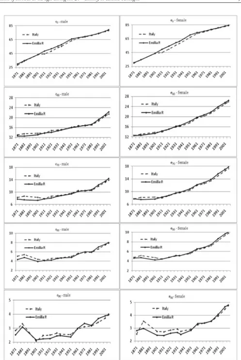
Figure 1 shows the evolution of life expectancy at birth and at certain adult and old ages5, in Emilia Romagna and Italy, during the period 1871-2007. The comparison between regional and national values, in terms of life expectancy at birth, shows a similar pattern for both genders for the years before 1901 and after 1971. In the long period between these two years, a better overall degree of survival is witnessed in the region than in the country as a whole. This fact can be explained by the sistematically lower regional infant and child mortality levels than the national ones. It seems that before and after mortality transition Emilia Romagna and Italy shared the same overall survival level, while during the transitional phase the region singularly anticipated the overall decline in mortality. With respect to elderly people, regional and national survival trends are quite different.
Regional and national life expectancies display similar trends for all adult and old ages, particularly from the beginning of the 20th century onwards. Emilia Ro-magna was at a disadvantage compared to Italy during the early decades, showing lower values at all ages because of the worse living conditions in Italian northern regions (Bellettini, 1980; Del Panta, 1984; Caselli and Egidi, 1980). As time went by, survival improved faster in the region than in the nation, and Emilia Romagna life expectancies rose above those for Italy as a whole from 1931 on for women, and from 1981 on for men. In other words, both men and women in Emilia Ro-magna have achieved better standards of living than in Italy as a whole, although women did so nearly fifty years earlier than men. The evolution of life expectan-cies at the end of the 19th century shows a peculiar profile not only for Emilia Romagna but for Italy too: at first there was an appreciable increase in survival for people aged 80-89, but this was followed by a clear decline. This particular as-pect has encouraged a more in-depth analysis, in order to understand whether the observed evolution really reflects a particular survival pattern during those years, or whether it was partly due to the widely acknowledged misreporting of deaths and/or population figures during that historical period. The results obtained are described in a forthcoming paper6.
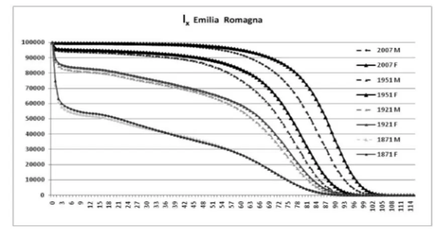
The profound changes in the evolution of survival can be seen in Figure 2, where the distribution of life table survivors (lx,) is shown by gender for the years
prior to the beginning of transition (1871), almost at the beginning thereof (1921), nearly at the end (1951) and in the post-transitional phase (2007).
5 The decision to compute life expectancy at 60, 70, 80 and 90 years was only one of the possible options available, and was taken in order to focus attention on the “elderly condition” over such a long time-span.
Figure 1 – Life expectancy at various ages – Emilia Romagna and Italy (1871-2007).
High levels of infant mortality shape the 1871 and 1921 curves, and still appear in 1951, while in 2007 the rectangularization of the survivors curve is clearly visi-ble. Gender differences are noticeable from 1921 on, and become more evident in 1951 and, above all, in 2007.
Figure 2 – Survivors lx by gender in 1871, 1921, 1951 and 2007.
TABLE 3
Median age at death and survivors at 65, 75, 85, 95 years by gender
1871 1921 1951 2007 Median age M 18.34 63.76 72.39 82.20 F 21.38 66.46 76.14 87.20 l65 M 21812 47861 67695 87922 F 21776 52540 77084 93050 l75 M 10005 24999 41796 72254 F 9792 29637 53930 84140 l85 M 1699 4332 10200 38884 F 1782 6503 17838 59195 l95 M 50 83 263 5886 F 77 229 937 14946
The progressive postponement of death to higher ages is also evident from the substantial rise in both median age and survival at elderly ages (Table 3). One half of the whole fictitious cohort had already died at the age of 18 years (males) or 21 (females) in 1871, whereas the same happened at 82 and 87 years, respectively, in 2007. Great changes in elderly survival are appreciable after the Second World War, and particularly nowadays: nearly 10% out of 100,000 newborns died before 65 years of age (both genders), while 39% and 59% (male and female respec-tively) were still alive at the age of 85.
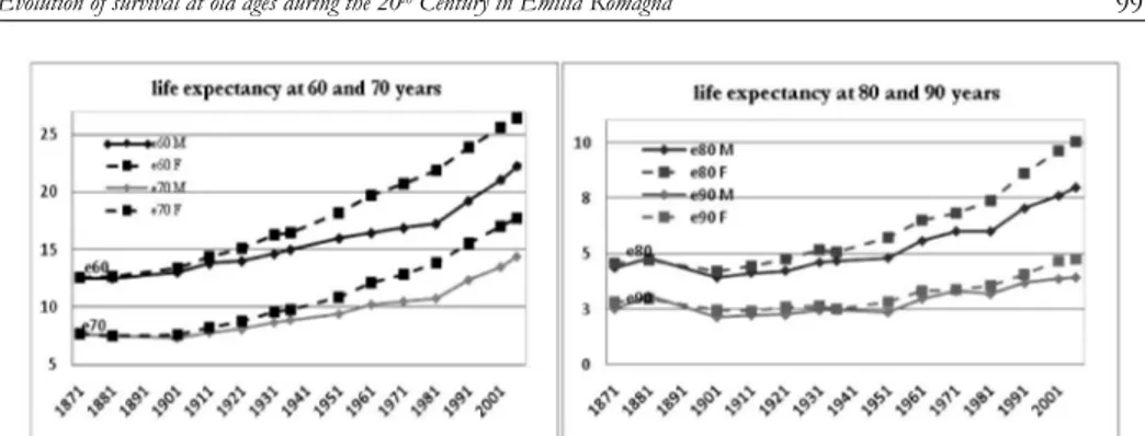
The analysis of life expectancy trends in Emilia Romagna shows that there are no particular signs either of gender differences or of any increase in residual life for people aged 60 years or over, until the initial years of the 20th century (see Figure 3). On the contrary, octogenarians and nonagenarians experienced a re-duction in life expectancy at the beginning of the last century.
Figure 3 – Life expectancy at 60, 70, 80 and 90 years by gender (1871-2007).
Later, towards the end of the First World War, residual life and gender differ-entials started to increase, slowly at first and then at a faster pace from 1951 on (see Figure 4).
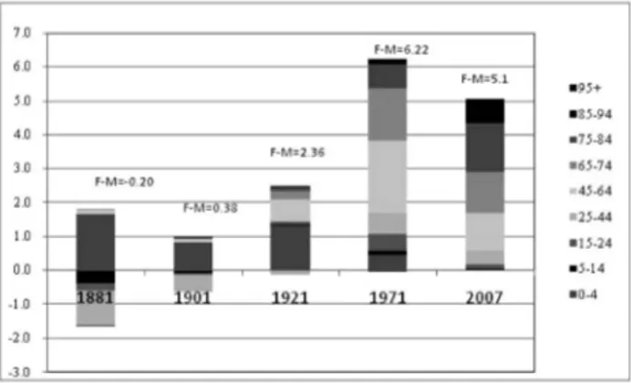
Figure 4 – Life expectancy at birth, differential by gender (F-M).
The rise in life expectancy was first witnessed for “younger” ages (60 and 70 years) and for women. In the latter case, life gains remained rather steady for all ages over the course of time, and they became more relevant from 1981 on, due to the adoption of healthier life styles, the spread of disease prevention, and im-provements in the early diagnosis of illnesses (Lipsi and Caselli, 2002; De Simoni and Lipsi, 2005). As far as males are concerned, the pace of growth was slower and only caught up with that of females at the beginning of the 1980s. A reduc-tion in gender differentials, particularly for e60, emerges from that period on. This fact is probably due to the growing similarity in male and female life styles as a consequence of women’s increased participation in the labour market together with their greater use of alcohol and tobacco, on the one hand, and of the adop-tion of healthier life styles for men, on the other hand.
3.2. Measuring the contribution of age to the rise in survival
Further evidence of the increasing importance of old age to the upward trend in survival can be obtained by decomposing the difference in life expectancy at
birth between time t1 and t2 according to the contribution due to the different age spans7.
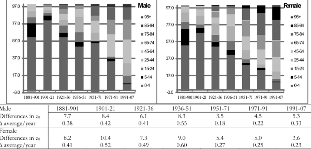
The analysis is performed for each gender separately, and the measures are ex-pressed both as fractions of years of life and as percentage contributions. If e0 displays an upward trend, positive values in Figure 5 reflect the positive contribu-tion to the difference in life expectancy between times t1 and t2, due to the decline in mortality of the different age groups. Conversely, negative values on the graphs underline a decline in survival for the age groups they belong to.
-3.0 17.0 37.0 57.0 77.0 97.0 1881-9011901-21 1921-36 1936-51 1951-71 1971-91 1991-07 Male 95+ 85-94 75-84 65-74 45-64 25-44 15-24 5-14 0-4 -3.0 17.0 37.0 57.0 77.0 97.0 1881-9011901-21 1921-36 1936-51 1951-71 1971-91 1991-07 Female 95+ 85-94 75-84 65-74 45-64 25-44 15-24 5-14 0-4 Male 1881-901 1901-21 1921-36 1936-51 1951-71 1971-91 1991-07 Differences in e0 7.7 8.4 6.1 8.3 3.5 4.5 5.3 ∆average/year 0.38 0.42 0.41 0.55 0.18 0.22 0.33 Female Differences in e0 8.2 10.4 7.3 9.0 5.4 5.0 3.6 ∆average/year 0.41 0.52 0.49 0.60 0.27 0.25 0.23
Figure 5 – Percentage contributions of different age groups to the increase in life expectancy for men and women in different time periods.
So far, reference has constantly been made to life expectancy at birth rather than to life expectancy at other adult or old ages, in order to evaluate increases in survival over time. Indeed, in the long run the tried-and-tested substantial varia-tions in e0 synthesize the strong changes in the structure of mortality, by sex and age, that Emilia-Romagna region, like all other Italian areas, has experienced be-tween the last decades of the nineteenth century and the present day. These changes are undoubtedly related to three distinct phases in the decline of mortal-ity: (a) a consistent rise in the number of years lived, due to increasing infant and child survival, until the Second World War; (b) a subsequent and continuous in-crease in the numbers of years lived, linked to adult lifespans up until the ̦70s; (c) an unespected positive contribution in survival from old people, of 65 years of age and above, that began in the 1980s.
A number of substantial gender differences emerge during the course of this long period of evolution. After the Second World War, female gains come earlier and are more substantial than those for men. The contribution of the 65 and
7 When dealing with decomposition methods in life expectancies, our main references are to Pol-lard’s works (1982, 1983, 1988), together with previous and subsequent literature (Arriaga, 1984, United Nations, 1985; Leridon and Toulemon, 1997; Ponnapalli, 2005). We applied different meth-ods that yielded comparable results.
above age group to the difference in life expectancy at birth amounts to 0.1 of a year in 1881-1901 with a total gain of more than than 8 years in e0; it remains
sta-ble at about 1 year until 1950, and subsequently rises to 2 years (out of a total gain of 5.4) in 1951-1971, 2.6 in 1971-1991, and 2.2 (out of 3.6 years) in 1991-2007.
In the case of males, it is possible to discern a slower trend in the rise in sur-vival, and the total gain in terms of years is not yet comparable to that of women, although during the last decade the male gain in e0 has been greater than that of
its female counterpart.
Figure 6 shows the contributions of the various age groups to the differences in life expectancy at birth between women and men for the four periods that rep-resent the several phases in the long trend evolution of mortality profiles.
It is noteworthy that in historical periods (that of 1881 and to a lesser extent that of 1901) when the difference in e0 between genders was practically negligible, the female disadvantage in terms of survival was mainly discernable in the young-est and reproductive age groups.
Figure 6 – Contributions (in fraction of years) of the different age groups to the male-female differ-ence in life expectancy at birth.
From 1921 onwards, the advantage of women over men was increasingly ap-preciable. Positive contributions confirm that the gender gap is largely due to the adult and old-age groups.
3.3. The evolution of longevity
As shown in the previous subsection, the on-going transition in mortality is characterized by considerable changes in survival patterns. So far these changes have been measured by such indicators as life expectancy at different ages, prob-abilities of death and of survival, and age-specific death rates. All these variables are suitable measures of survival conditions; however, as far as ageing is concerned, they have the disadvantage of requiring the arbitrary selection of age limits.
Life expectancy at birth is without any doubt one of the best indicators both of infant and overall survival, although it loses its effectiveness when the question is
elderly survival in low-mortality populations. In the early stages of demographic transition, a considerable contribution to the increase of life expectancy at birth is given by the great reduction in infant and childhood mortality. On the contrary, whilst as the transition progresses, the most relevant reduction in mortality con-cerns adult and old ages, which exert only a marginal effect on e0. So, when the interest focuses on the analysis of longevity and its evolution, it is a better idea to consider measures that are more sensitive to changes in adult survival, such as late modal age at death and the related indicators (Kannisto, 2001; Cheung et al., 2005; Cheung and Robine, 2007).
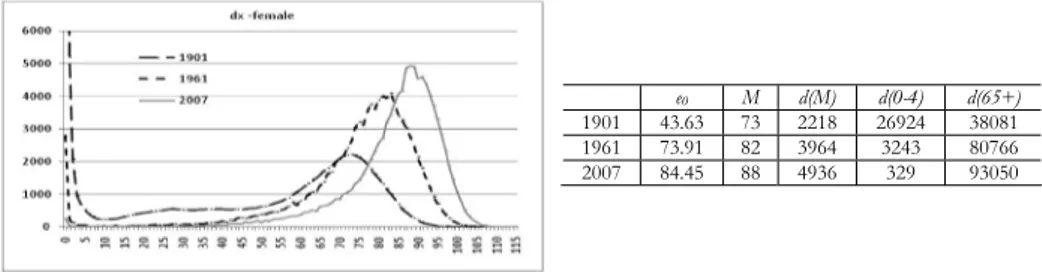
Figure 7 shows the evolution in the distribution of deaths, together with some survival indicators, for Emilia Romagna’s female population at the beginning and in the middle of the 20th century, and at the beginning of the 21st century. It is possible to appreciate the substantial drop in infant and childhood mortality, and the remarkable increase in the number of deaths among the elderly (65+) during the first half of the century. Life expectancy at birth (43.63 years) was very differ-ent from late modal age at death (73 years) in 1901, due to the fact that a great amount of deaths (nearly 26% of the total) were concentrated in the first five years of life. Since then, the reduction in infant and child mortality has narrowed the gap between the two indicators in the mid 20th century; while nowadays this difference is really small and the two indicators tend to evolve in a parallel fash-ion. Current increases in life expectancy at birth are now mainly due to the great gains achieved in survival among the adult and elderly population. Therefore, late modal age at death becomes a suitable indicator in the analysis of rising longevity.
Figure 7 – Distribution of life table deaths in 1901, 1961 and 2007 and values of life expectancy(e0), late modal age at death (M), modal number of deaths (d(M)), infant (d(0-4)) and elderly (d(65+)) deaths in the same years. Emilia Romagna – female.
Modal age is sometimes difficult to be detected due to the irregularities that life table death series dx show near the mode: several distinct maximum points, or a
flat-topped peak, may be observed (Cheung and Robine, 2007). As observed by Lexis (1878), the distribution of deaths above the mode can be summarized by the righthand side of a normal distribution. Lexis also suggested that, were it pos-sible to avoid all untimely deaths, the distribution of deaths would follow a nor-mal distribution also for those ages below the mode. It means that if all elderly deaths were “normal” they would be distributed according to “the error law”. So, we used a scaled normal model in order to obtain a single estimation of modal
e0 M d(M) d(0-4) d(65+)
1901 43.63 73 2218 26924 38081 1961 73.91 82 3964 3243 80766 2007 84.45 88 4936 329 93050
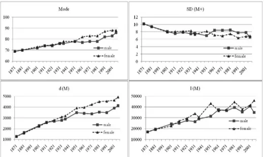
age at death8. The estimated modal age at death is shown in Table 4 and Figure 8, together with other indicators related to the mode, chosen to describe the evolu-tion of longevity in Emilia Romagna. These indicators were calculated using the unfitted life table death series dx.
Late modal age at death (M) increased steadily and indeed noticeably during the whole period: at the beginning it is equal to 69 years for both genders, while at the end it reaches 86 years for men and 88 for women, with an increase of nearly 25% and 28% respectively. Men and women shared a common path in modal age at death growth up until the Second World War. Thereafter the female indicator rose more substantially, reaching and going beyond the threshold of eighty years during the fifties, nearly three decades before the male indicator did.
According to Kannisto (2001), late modal age at death (M) and the standard deviation above it (SD(M+)) provide a satisfactory account of adult longevity un-der a given mortality regime. In Emilia Romagna the standard deviation above the mode decreases steadly in the first decades for both genders, then it follows an unchanging trend in spite of several fluctuations around the value 8 for men, while it tends to decrease after the Second World War for females, reaching val-ues of around 6.5, and showing a different pattern between genders. Finally, for the last year of observation these patterns tend to converge, with a slightly higher value for females than for males.
TABLE 4
Modal age (M), standard deviation above the estimated mode (SD(M+)), deaths d(M) and survivors l(M) at modal age 1871 1881 1901 1911 1921 1931 1936 male M 69 70 72 74 74 76 76 SD(M+) 10.19 9.44 8.12 7.54 7.89 7.47 7.62 d(M) 1266 1638 2293 2579 2682 2763 2883 l(M) 17065 19586 24427 25159 27588 26411 28912 female M 69 70 73 74 75 76 78 SD(M+) 10.16 9.41 7.97 8.10 8.13 8.31 7.32 d(M) 1274 1587 2218 2565 2795 3084 3192 l(M) 17017 19243 22634 27136 29637 33978 30480 1951 1961 1971 1981 1991 2001 2007 male M 78 77 78 78 82 83 86 SD(M+) 7.01 8.48 8.46 8.49 7.77 7.81 6.57 d(M) 3498 3423 3381 3535 3485 3901 4142 l(M) 31555 37560 36614 39564 35328 40606 34970 female M 78 82 83 83 87 88 88 SD(M+) 8.18 7.17 6.94 7.47 6.39 6.80 6.95 d(M) 3913 3964 4242 4506 4536 4646 4936 l(M) 43384 36620 37713 44720 38076 41664 46085
8 In order to estimate the parameters characterizing the scaled normal distribution., a nonlinear least squares method is used from 5 years before the observed modal age at death to the tail of the curve. The choice of setting the regression to start exactly 5 points before the observed mode is motivated from a previus sensitivity analysis showing that this choice generally yields the best model fitting. Indeed, the R2 values vary from a minimum of 0.9853 to a maximum of 0.9997, showing that the scaled normal models accurately approximate the distributions of observed dx.
The amount of deaths at modal age d(M), representing the concentration of human lives ending in the single year of age M, grew during the observational pe-riod: it was approximately equal to 1,400 per 100,000 newborn in 1871 for both genders, and it had reached nearly 4,100 men and 4,900 women by 2007. This progressive concentration of deaths in a single age class does not occur uniformly over the course of time, but it alternates periods of stagnation or reversal with pe-riods of rapid increase. The rise in the number of deaths at modal age is obvi-ously associated to a reduction in the number of individual lives that end before and after this age. During the whole observational period, the most important contribution to the concentration of deaths around the mode was undoubtedly made by the radical reduction in untimely deaths, as witnessed by the increasing number of survivors at modal age l(M), which is equal to deaths over the modal age M (d(M+)). The number of survivors at modal age was nearly 17,000 out of 100,000 newborn for both genders, while in 2007 it is about 35,000 for males and approximately 46,000 for females. However, even if the global trend is rising, it is possible to note the swinging evolution of the indicator. So if we compare the continuous increase in the number of deaths gathered at the mode (d(M)) with the number of deaths gathered at and above M (d(M+)), we can observe that sometimes individual life durations ending at and above the mode are more com-pressed.
Figure 8 – Modal age (M), standard deviation above the estimated mode (SD(M+)), deaths d(M) and survivors l(M) at modal age.
The number of survivors at modal age also enables us to evaluate the propor-tion of lives that end under the hypotethical normal curve that can be drawn if the distribution of deaths over the mode is applied on the lefthand side. This per-centage represents the so-called lives of full length (LFL) under a given mortality
schedule; this means that the level of mortality in 1871 allowed nearly 34% of the population to reach a life of full length, while that in 2007 allowed more than 90% of the female population to live a LFL. So it seems that nowadays female survival has reached optimal standards in Emilia Romagna where nearly the whole population shares a “normal” length of life, while only 10% of a lifetable’s newborns are involved in an untimely death.
Demographers tend to differ on the question of the changes in senescent mor-tality that are responsible for increasing longevity. The contrasting theories are mainly that of the compression of mortality theory and that of the shifting mor-tality scenario (Fries, 1980; Myers and Manton, 1984; Kannisto, 1996; Bongaarts, 2005; Canudas-Romo, 2008; Robine et al., 2008). According to the first theory, an increase in late modal age is accompanied by a reduction in the dispersion of in-dividual life durations ending above the mode. This fact means that the inin-dividual life durations ending above the mode are compressed into a smaller age range above the mode. On the contrary, increasing values of late modal age associated with no change in the dispersion suggests the shifting mortality scenario, whereby the whole distribution of individual life durations ending above the mode slides proportionally to higher ages.
At a first glance, Emilia Romagna data fail to display the presence of a linear relationship between the steady increase in M and the evolution in SD(M+). The continous postponement of modal age at death toward higher ages is not always associated with a reduction in the dispersion of deaths over this age, therefore, there are no steady signs that the increase in longevity in the region is always as-sociated with a compression of mortality in a shorter age span. However, by comparing the steady increase in the number of deaths at the mode with the number of deaths gathered at and above it, we have observed that in certain peri-ods, individual life durations ending at and above the mode are compressed to a greater degree.
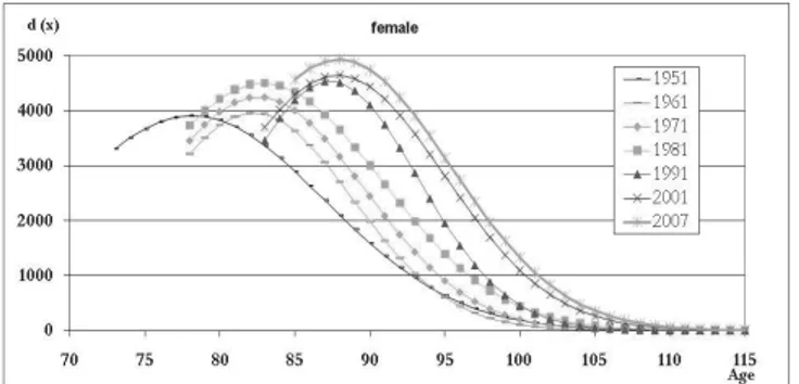
The observation of the normal death profiles (Figure 9) underlines the previ-ously-shown increase in modal age at death associated with a noteworthy rise in the modal number of deaths. When the modal age at death moves ahead (as hap-pened, for example, between 1981 and 1991 for both genders) it is generally pos-sible to observe a reduction in the standard deviation of deaths above the mode, together with a decrease in the number of survivors that reach the new modal age at death (see Table 4) . In the following years, the modal age at death normally remains steady and both the dispersion above the mode and the survivors at mo-dal age grow. It seems that the increase in longevity initially pertains to an élite before subsequently spreading throughout the wider population.
In order to provide a more in-depth analysis of elderly survival increase in the region, we have focused on the female population, with women anticipating their male counterparts in terms of increases in longevity. In the period following the Second World War, when the greatest changes in longevity occurred, we can see two clear increases in modal age at death which divide the evolution of longevity into three distinct steps (Figure 10).
Figure 9 – Distribution of death fitted with a scaled normal distribution (1871-2007).
Figure 10 – Female distribution of death fitted with a scaled normal distribution (1951-2007).
In order to evaluate the evolution of life table death curves and to understand how the mortality law has changed, it is also useful to analyze the trend of the two parameters α and β of the logistic function that define µx, the force of mortal-ity at each age x. The first one, α, varies with the level of mortalmortal-ity, while β meas-ures the rate of increase in mortality with increasing age (Figure 11).
Figure 11 – Paremeters α and β of the logistic model- female (1951-2007).
The level parameter shows a clear downward evolution during the period of observation, with the exception of 1961. The slope parameter β appears less vari-able and alternates between slowing down, remaining steady and increasing. Dur-Years alpha beta
1951 0.061 0.123 1961 0.075 0.118 1971 0.036 0.125 1981 0.017 0.133 1991 0.009 0.137 2001 0.006 0.138 2007 0.003 0.146
ing those periods in which the level of mortality decreases and the rate of increase grows, we can observe a compression in mortality, while when the slope parame-ter also decreases, there is an expansion in mortality. Finally, when the level slows down and the slope remains steady we have a shift in mortality.
The first increase in modal age at death occurs between 1951 and 1961, and consists of a gain of four years. The number of deaths at modal age remains steady, while there is an appreciable reduction in the dispersion indicator (see Ta-ble 4). The level of mortality increases slightly, while the slope drops down show-ing a certain degree of expansion in mortality. Durshow-ing the period 1961-1981 the modal age at death does not vary, the parameter α decreases, while β grows. This is a period of compression of mortality, with an increasing number of individuals reaching modal age at death (due to the increased avoidance of premature deaths), and where it seems that the growth in life span length has finally ceased. This remains true until the eighties, when modal age at death rises again, amount-ing to another gain of four years. Between 1981 and 1991 it is possible to observe a clear shift in senescent mortality as suggested by the slow down in the level pa-rameter and by the constancy of the mortality slope value. Finally, the last two decades of the observation period ending in 2007 are characterized by another phase of compression of mortality associated with a further increases in the num-ber of survivors at modal age at death. The reasons for the unique trend are strongly linked with the evolution of mortality by cause, a topic that lies beyond the scope of this paper, but will be the main focus of future study.
In conclusion, the figures for Emilia Romagna seem to show that the recent regional evolution in longevity has not followed one single pattern, but consists of alternate phases, some that conform to compression mortality theory, and oth-ers corresponding to the shifting mortality scenario. It is obvious that regional data do not enable us to draw any general conclusions, and it is still not possible to tell whether regional population life length has already reached its maximum limit; only future observations will shed the necessary light on the evolution of this intriguing aspect.
4. CONCLUSIONS
This paper merely constitutes a preliminary, albeit essential part, of a larger re-search project aimed at: a) the definition of some indicators of elderly survival by gender at the regional and provincial levels, that will permit the analysis of lon-gevity evolution in Emilia Romagna and of its territorial distribution; b) the analy-sis of mortality by cause of death, mortality and morbidity profiles and their re-cent evolution by age; c) the spatial mapping of longevity linked with the prevail-ing causes of death.
Starting from the construction of period life tables according to a standardised procedure, the present paper develops three main topics, centred on the first ob-jective of the main research project: a descriptive analysis of the long-term evolu-tion of elderly survival, from the beginning of demographic transievolu-tion to the
pre-sent day; an in-depth study of the ages that mostly contributed to the increase in survival during the different transitional stages; an investigation of the evolution of longevity.
The study of the evolution of mortality in Emilia Romagna has revealed the remarkable gains achieved by the elderly population, and particularly by females, and has highlighted the presence of better conditions for survival in the region than in the country as a whole over recent decades. The different pattern detected in Emilia Romagna compared to Italy as a whole is a good reason to pursue a bet-ter understanding of the overall national situation. Regional studies are particu-larly important in realities such as the Italian one, where regions are characterized by very different demographic behaviours. It is widely acknowledged that even though regions are exclusively administrative subdivisions of the national terri-tory, regional data can explain the major part of the national variability of demo-graphic phenomena. This fact encourages and underlines the relevance of the de-velopment of regional analysis in Italy.
The results we have obtained also suggest that at least in the case of the XIXth century life tables, a specific in-depth analysis is required in order to test the qual-ity of original data and to study the peculiar pattern of elderly mortalqual-ity.
The second topic we have focused on has underlined how recent increases in life expectancy at birth have been mostly due to the improvement in survival at adult and old ages as of the 1970s. Once again, female behavior anticipates that of men, even though in the last decade the values for the two genders have tended to move closer together.
Finally, in the third part of the paper we have shown how longevity increased during the period in question. During the years after the Second World War, we also observed that the steady increase in the late modal age at death does not fol-low one single pattern, but it alternates phases that meet with compression mor-tality theory, with phases that correspond to the shifting mormor-tality scenario.
As we have already said, the continuation and extension of the research project should be devoted to the study of elderly mortality by cause of death9. Figures for the distribution of death by cause and by age at the sub-regional level are only available for the last decades of 20th century onwards. This kind of approach will improve our understanding of the observed survival evolution, and will shed some light on the peculiar aspects of regional mortality profiles by cause.
Although we can not affirm for sure that Emilia Romagna’s elderly population will continue to increase in the near future, the great majority of the population in adult ages and the current level of survival would suggest that in the near future local government will continue to face all those problems associated with an age-ing population. Such problems as medical expenditure and social welfare services will undoubtedly be of particular importance. Italian welfare is still centred on the role played by families, who are the principal providers of assistance and support to needy household members. Women in particular have always been the
9 A spatial analysis of elderly mortality by cause of death in Emilia Romagna has been performed in Miglio, Marino, Rettaroli, Samoggia (2009, forthcoming).
pal players in this process, due both to their particular devotion to the wellbeing of the family members, and to their relatively scarce partecipation in the labour force. Policy makers have to consider that the number of female workers in Italy is rising nowadays, and will continue to rise in the near future, leaving a growing number of family members without the help they need. This fact is particulary true in Emilia Romagna: an Italian region with one of the highest level of female employment and one of the highest proportions of elderly citizens. Assistance to the elderly has been increasingly provided by immigrant carers who until now have filled the gap between the rising number of eldely people that need care and the paucity of public assistance services. Even if immigrant carers have resolved this crucial problem for the time being, it is hard to say whether the Italian gov-ernment can continue to avoid the growing demand for public support for fami-lies with elderly members.
Department of Statistical Sciences “P. Fortunati” ROSELLA RETTAROLI
University of Bologna GIULIA ROLI
ALESSANDRA SAMOGGIA
REFERENCES
E.E. ARRIAGA,(1984),Measuring and explaining the change in life expectancies, “Demography”, 21,
pp. 83-96.
A. BELLETTINI, (1980), Il quadro demografico dell’Italia nei primi decenni dell’unità nazionale, in “Atti del L Congresso di Storia del Risorgimento italiano”, Bologna, Istituto per la Storia del Risorgimento italiano, pp. 445-500.
J. BONGAARTS, (2005), Long-range trends in adult mortality: models and projection methods, “Demog-raphy”, 42(1), pp. 23-49.
V. CANUDAS-ROMO,(2008), The modal age at death and the shifting mortality hypothesis, “Demo-graphic Research” 19(30), pp. 1179-1204.
G. CASELLI,(1990), Mortalità e sopravvivenza in Italia dall’Unità agli anni ’30, in SIDeS, Popola-
zione, società e ambiente. Temi di demografia storica italiana (secc. XVII-XIX), Bologna,
CLEUB, pp. 275-309.
G. CASELLI, (2007), Mortalità degli adulti e differenze di genere nella prima fase della transizione
sani-taria, in M. Breschi, L. Pozzi (eds), Salute, malattia e sopravvivenza in Italia tra ’800 e ’900,
Udine, Forum, pp. 293-310.
G. CASELLI, R. CAPOCACCIA, (1989), Age, period, cohort and early mortality: an analysis of adult
mor-tality in Italy, “Population Studies”, 43, pp. 133-153.
G. CASELLI, V. EGIDI,(1980), Le differenze territoriali di mortalità in Italia. Tavole di mortalità
provin-ciali (1971-72), n. 32, Istituto di Demografia dell’Università “La Sapienza” di Roma, pp.
1-167.
G. CASELLI, R.M. LIPSI, (2006), Survival differences among the oldest old in Sardinia: who, what, where,
and why, “Demographic Research”, 14(13), pp. 267-294.
S.L.K. CHEUNG, J.M. ROBINE(2007), Increase in common longevity and the compression of mortality: The
case of Japan, “Population Studies”, 61,1, pp. 85-97.
S. L. K. CHEUNG, J.M. ROBINE, E.J.C. TU, G. CASELLI,(2005),Three Dimensions of the Survival Curve: Horizontalization, Verticalization, and Longevity Extension, “Demography”, 42(2), pp. 243-
L. DEL PANTA, (1984), Evoluzione demografica e popolamento nell’Italia dell’Ottocento (1796-1914), Bologna, CLUEB.
L. DEL PANTA, L. BELOTTI, D. CALÒ,(2009), Elderly mortality in italian regions at the beginning of the
health transition (1881-1921), “Statistica” , forthcoming.
A. DE SIMONI, R.M. LIPSI, (2005), La mortalità per causa in Italia nell’ultimo trentennio. Tavole di
mor-talità 1971, 1976, 1981, 1986, 1991, 1996 e 2000. Fonti e strumenti, Dipartimento di
Scienze Demografiche, n. 6, Roma.
J. F. FRIES,(1980),Aging, natural death and the compression of morbidity, “New England Journal of Medicine”, 303(3), pp. 130-135.
B. GOMPERTZ, (1825), On the nature of the function expressive of the law of human mortality, and on
the mode of determining the value of life contingencies, “Philosophical Transactions of the Royal
Society”, 115, pp. 513-519.
S. HORIUCHI, A.J. COALE,(1990), Age patterns of mortality for older women: an analysis using the
age-specific rate of mortality change with age, “Mathematical Population Studies”,2, pp.
245-267.
S. HORIUCHI, J.R. WILMOTH, (1998), Deceleration in the Age Pattern of Mortality at Older Ages, “Demography”, 35(4), pp. 391-412.
V. KANNISTO,(1996),The Advancing Frontier of Survival: Life Tables for Old Age,Odense Mono-graphs on Population Aging, 3. Odense University Press, Odense, Denmark.
V. KANNISTO, (2000), Measuring the Compression of Mortality, “Demograpic Research”, vol. 3/6, pp. 1-24.
V. KANNISTO,(2001),Mode and Dispersion of the Length of Life,Population: An English Selec-tion, 13(1), pp. 159-171.
V. KANNISTO, J. LAURITSEN, A. R. THATCHER, J. W. VAUPEL, (1994), Reductions in Mortality at
Ad-vanced Ages: Several Decades of Evidence from 27 Countries, “Population and Development
Review”, 20(4), pp. 793-810.
H. LERIDON, L. TOULEMON, (1997), Démographie. Approche statistique et dynamique des populations, Economica, Paris.
W. LEXIS, (1878), Sur la Durée Normale de la Vie Humaine et sur la Théorie de la Stabilité des
Rap-ports Statistiques, “Annales de Démographie Internationale” 2(5), pp. 447-460.
R. M. LIPSI, G. CASELLI, (2002), Evoluzione della geografia della mortalità in Italia. Tavole provinciali e
probabilità di morte per causa, Dipartimento di Scienze Demografiche, Roma.
D.R. MCNEIL, T.J. TRUSSELL, J.C. TURNER,(1977),Spline interpolation of demographic data, “Demog-raphy” 14(2), pp. 245-252.
R. MIGLIO, M. MARINO, R. RETTAROLI, A. SAMOGGIA, (2009), Spatial analysis of longevity in a
North-ern Italian region, Paper accepted for the Population Association of America (PAA)
Meeting 2009.
G.C. MYERS, K.G. MANTON, (1984), Compression of mortality: myth or reality?, “The Gerontolo-gist”, 24, pp. 346-353.
J.H. POLLARD (1982), The expectation of life and its relationship to mortality, The Journal of
the Institute of Actuaries, 109, Part 2(442), pp. 225-240.
J.H. POLLARD (1983), Some methodological issuesin the measurement of sex mortality patterns, in Lo-pez A.R., and L.T. Ruzicka (eds.), Sex differentials in mortality: trends, determinants and
conse-quences, Australian National University, Canberra.
J.H. POLLARD (1988), On the decomposition of changes in expectation of life and differen-tials in life expectancy, Demography, 25, 2, pp. 265-276.
K.M. PONNAPALLI, (2005), A comparison of different methods for decomposition of changes in
expecta-tion of life at birth and differentials in life expectancy at birth, “Demographic Research”, 12(7),
L. POZZI, (2000), La lotta per la vita. Evoluzione e geografia della sopravvivenza in Italia fra ’800 e
’900, Udine, Forum.
J.M. ROBINE, S.L.K CHEUNG, S. HORIUCHI, A.R. THATCHER, (2008), Is There a Limit to the
Compres-sion of Mortality?, paper presented at the “Living to 100 and Beyond” Symposium, Orlando,
Fla, January 7-9.
G. ROLI,(2008),An adaptive procedure for estimating and comparing the old-age mortality in a long
his-torical perspective: Emilia-Romagna, 1871-2001,“Quaderni di Dipartimento” - Serie
Ricer-che 2008(8).
A. R. THATCHER,(1992), Trends in Numbers and Mortality at High Ages in England and Wales, “Population Studies”, 46, pp. 411-426.
A. R. THATCHER,(1999),The Long-Term Pattern of Adult Mortality and the Highest Attained Age, “Journal of the Royal Statistical Society”, Series A (Statistics in Society)”, 162(1), pp. 5-43.
A.R. THATCHER, V. KANNISTO, J.W. VAUPEL, (1998), The Force of Mortality at Ages 80 to 120. Odense, Denmark: Odense University Press.
UNITED NATIONS,(1985), World population trends, population development inter-relations and
popula-tion policies. 1983, Monitoring report, vol.I, Populapopula-tion trends, ST/ESA/Ser. A./93,
United Nations, Dept. of International and Economic and Social Affairs, New York. J.R. WILMOTH, K. ANDREEV, D. JDANOV, D.A. GLEIwith the assistance ofC. BOE , BUBENHEIM M.,
PHILIPOV D., SHKOLNIKOV V., VACHON P.(2007),Methods Protocol for the Human Mortality
Da-tabase, (Version 5), http://www.mortality.org.
SUMMARY
Evolution of survival at old ages during the 20th Century in Emilia Romagna
The paper presents some preliminary results of a project devoted to the analysis of adult and elderly mortality evolution in a Northern Italian region, Emilia Romagna, during the health transition. Starting from the construction of 14 period life tables (1871-2007) according to a standardised procedure, the paper develops three main topics: a descriptive analysis of the long-term evolution of elderly survival from the beginning of demographic transition to the present day; an in-depth study of those ages that have made the greatest contribution to the increase in survival during the various different transitional stages; an investigation of the evolution of longevity.