E FISCHE
CORSO DI DOTTORATO XXIII CICLO
Study of Kaon semileptonic decays on the lattice using
twisted-mass fermions and stochastic techniques for light-meson
propagators
Lorenzo Orifici
A.A. 2010/2011
Docente Guida/Tutor:
Dott. S. Simula & Prof. V. Lubicz Coordinatore:
I would like to thank the Roma Tre lattice group which I joined for this PhD thesis work and without whom all this work would have not been possible. A special mention for Silvano Simula is in order: his help, his constant support and his patience during our discussions have been of fundamental importance for obtaining the results of this work. I wish to thank him very much for all his teachings. I am also very grateful to Roberto Frezzotti for his very precise and insightful corrections to the present thesis. Finally I would like to thank also my colleagues Stefano Di Vita and Francesco Sanfilippo for useful discussions as well as for their important suggestions during the writing period of this thesis. Last, but not least, I would like to thank the INFN ApeNext supercomputing center and the Ape group for keeping the ApeNext machines always at work.
List of Figures vii
List of Tables ix
Introduction xi
1 Flavour Physics 1
1.1 The Standard Model . . . 1
1.2 Cabibbo-Kobayashi-Maskawa matrix . . . 8
1.2.1 Definition & parametrization . . . 8
1.2.2 Experimental determination . . . 15
1.3 Leptonic and semileptonic meson decays . . . 20
1.3.1 Leptonic Kaon decays . . . 22
1.3.2 Semileptonic Kaon decays . . . 25
1.3.3 Ademollo Gatto theorem . . . 28
1.4 CP violation . . . 29
1.4.1 Weak CP violation . . . 31
1.4.2 Strong CP violation . . . 36
2 Lattice Quantum Chromodynamics 47 2.1 Quantum Chromodynamics . . . 47
2.2 Lattice gauge theories . . . 50
2.2.1 Gauge bosons action . . . 51
2.2.2 Fermionic Wilson action . . . 55
2.3 Improvement . . . 60
2.4.1 Automatic improvement . . . 65
2.4.2 Wilson Average and O(a) improvement . . . 66
2.4.3 Improved physics from tm-LQCD . . . 70
2.4.4 Local operator renormalization within mtm-LQCD . . . 73
2.5 Twisted boundary conditions . . . 74
2.5.1 Continuum definition . . . 74
2.5.2 Lattice implementation . . . 77
2.6 Numerical methods for Gauge theories . . . 79
2.6.1 Pure gauge theories . . . 80
2.6.2 Numerical methods for fermionic systems . . . 81
3 What has to be computed 85 3.1 Extracting information from LQCD . . . 85
3.1.1 Two–point correlation functions . . . 86
3.1.2 Three–point correlation functions . . . 90
3.2 Semileptonic Kaon decays . . . 91
3.2.1 The ratio and the double ratio method . . . 91
3.2.2 Semileptonic correlators & the all-to-all propagator . . . 97
3.2.3 Stochastic procedures for connected diagrams . . . 100
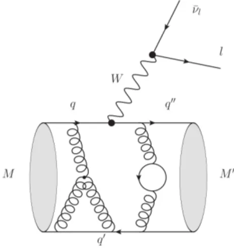
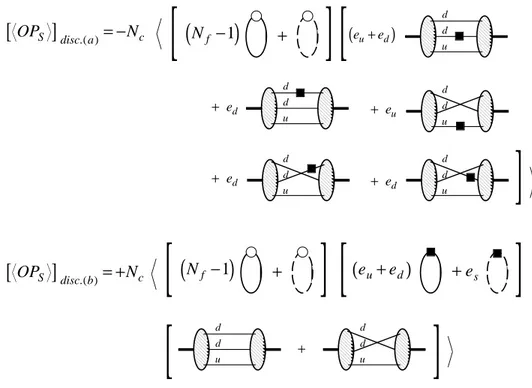
3.3 The road to the neutron EDM calculation . . . 103
3.3.1 Quark-Disconnected diagrams & all-to-all propagators . . . 104
4 Results 121 4.1 Simulation details . . . 122 4.2 Error analysis . . . 125 4.2.1 Statistical errors . . . 126 4.2.2 Jackknife analysis . . . 127 4.2.3 Bootstrap analysis . . . 128
4.3 Momentum dependence of the two–point correlation function . . . 129
4.4 Momentum dependence of the semileptonic form factors . . . 134
4.5 Fixing the strange quark mass . . . 139
4.6 Systematic errors . . . 143
4.6.1 Discretization errors . . . 143
4.7 Reaching the physical point . . . 148
4.7.1 Form factors structure . . . 148
4.7.2 Quenching of the strange quark . . . 155
4.8 Physical results: semileptonic form factors & Vus . . . 160
4.9 Present status of our stochastic technique . . . 161
Conclusions 169
1.1 Flavour mixing hierarchy . . . 12
1.2 Unitary triangle . . . 14
1.3 Leptonic decay prototype . . . 23
1.4 Semileptonic decay prototype . . . 25
1.5 K0 − ¯K0 mixing. . . 31
1.6 neutron EDM topology . . . 45
3.1 Kaon two–point function . . . 98
3.2 Kaon three–point function . . . 99
3.3 Connected topology . . . 106
3.4 Disconnected topology . . . 106
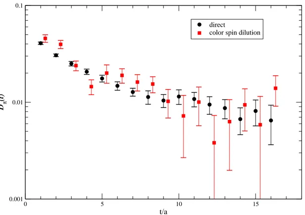
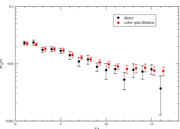
3.5 Direct V.S. color spin dilution method (π0) . . . . 111
3.6 Direct V.S. color spin dilution method (η′) . . . . 112
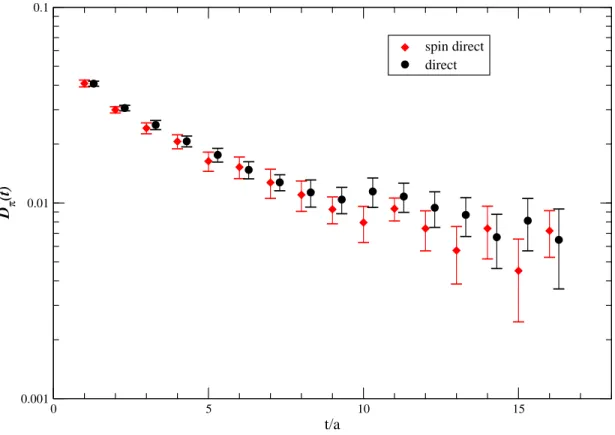
3.7 Spin–direct V.S. direct method (π0) . . . 115
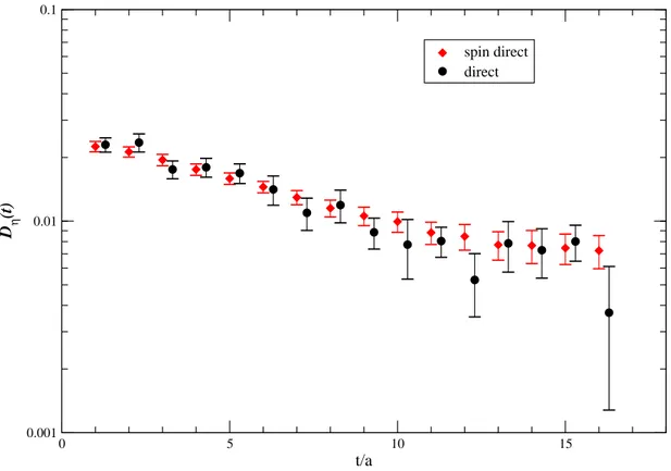
3.8 Spin–direct V.S. direct method (η′) . . . . 116
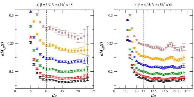
4.1 Light-light effective mass . . . 130
4.2 Strange-light effective mass . . . 131
4.3 Light-light energy . . . 133
4.4 Strange-light energy . . . 134
4.5 Scalar form factor (time) plateau . . . 135
4.6 Vector form factor (time) plateau . . . 136
4.7 Scalar form factor at qM AX2 (time) plateau . . . 138
4.8 Form factors momentum dependence . . . 140
4.9 Form factors M2 K dependence . . . 141
4.10 Form factors momentum dependence at MKref . . . 142
4.11 Discretization errors for f0(q2) at MKref . . . 144
4.12 Discretization errors for f+(q2) at MKref . . . 145
4.13 Finite size effects for f0(q2) at MKref . . . 146
4.14 Finite size effects for f+(q2) at MKref . . . 147
4.15 Scalar form factor fit quality . . . 156
4.16 Vector form factor fit quality . . . 157
4.17 ∆f comparison . . . 159
4.18 Scalar and vector form factors experimental comparison . . . 162
4.19 η′ disconnected diagrams (I) . . . . 164
4.20 η′ disconnected diagrams (II) . . . 165
1.1 Electroweak quantum numbers . . . 5
3.1 Dirac covariant’s quantum numbers . . . 89
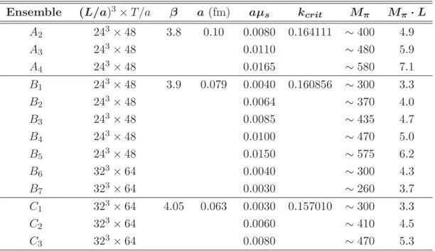
4.1 Gauge field configurations set up . . . 123
4.2 Time plateau . . . 137
4.3 Form factor’s parameters FSE . . . 148
4.4 Physical results . . . 160
Weak hadron decays are very interesting processes because measuring the decay widths for such processes allow to extract some of the fundamental parameters of the Standard Model of electroweak interaction [1]. In particular it is possible to extract the modulus of the elements of the Cabibbo–Kobayashi–Maskawa (CKM ) flavour mixing matrix [2;3], which describe the flavour sector of the Standard Model.
The needed theoretical quantity, thanks to which one can obtain from the exper-imental measure of a given decay the related CKM matrix elements, are standard perturbative computing and the form factors which parametrize the hadron matrix element relevant for the decay.
The strong interaction physics is described by means of the Quantum Chromody-namics (QCD) [4;5; 6]. It is known that QCD is a gauge theory characterized by the presence of the asymptotic freedom: the interaction’s coupling goes to zero as the en-ergy which describe the process become much greater than a characteristic scale of the theory, known as ΛQCD (≃ 1 GeV ). Conversely, in the low energy limit (E . ΛQCD), it
is no more possible to treat the interaction by means of perturbative methods because the coupling constant is O(1).
Lattice QCD (LQCD) [7] is a non-perturbative formulation of QCD based on first principles. In particular, it provides a peculiar regularization scheme in which the ultraviolet cut–off for momenta is given by the inverse of the lattice spacing; however, the specific importance of the lattice approach to QCD lies in the fact that it provides a systematic methodology via Monte Carlo simulations for carrying out quantitative calculations in the energy range in which it is not possible to perform perturbative estimates of the physical observables. This energy range overlaps with the energy scale characteristic of the weak hadron decays.
The processes which we are interested in are the ones in which a single hadron is present in both the initial and/or final state. These processes include leptonic de-cays, semileptonic decays and neutral meson oscillations. The study of processes with more than one hadron in the final state (for instance K → ππ decays) present greater difficulties within LQCD standards methods.
LQCD calculation exploit the deep analogy between the lattice formulation of quan-tum field theories (in euclidean space–time) and the statistical mechanic description of a physical system. In particular it is possible to use Monte Carlo simulation techniques. We would like to underline that LQCD allows a continuous improvement of the precision for the obtained results. The systematic error sources can, in fact, be kept under control using increased computational power, refined algorithms and improved techniques. Statistical errors can be reduced using bigger samples; discretization ef-fects get less relevant reducing the lattice spacing; finite volume efef-fects can be avoided increasing the lattice volume in which the quark and gluon’s dynamics is simulated.
The present computational power strongly constraints the possible quark masses which can be simulated in LQCD, and in particular we are obliged to use light quark masses which are heavier than physical ones; thus, in order to obtain physical predic-tions for the quantities of interest we have to fit the dependence of our observables with respect to the quark masses. Chiral Perturbation theory can express meson masses as a function of the (bare) quark masses and so in our simulations we have chosen to study the quantities of interest as a function of meson masses (in particular the Kaon and pion mass). The light physical meson extrapolations, called chiral extrapolations, are another source of systematic error which must be kept under control.
For heavy mesons, another limitation is present: on a lattice with spacing a it is possible to simulate only states with mass lighter than the theory cut-off, which is given by the inverse lattice spacing (π/a). If we want to predict something about hadrons heavier than the ones which can be simulated on the lattice we will have to employ extrapolation again, this time in the heavy hadron mass.
The target is to be able to simulate energy regions in which it is possible to apply effective descriptions of QCD and perform the extrapolations using their predictions. Chiral perturbation theory (ChPT) describe the limit of vanishing light u and d (and s if one is considering SU (3) ChPT) quark masses. Heavy quark effective theories (HQET, NRQCD) can instead describe the B and D meson physics. A combination of the two
theories (known as Heavy Mesons χPT) allow one to describe the decays of heavy to light hadrons; the subject of this work are the semileptonic kaon decays K → πlνl and
so we will limit our attention to SU (2) and SU (3) ChPT for extrapolating our form factors to the physical point.
In the lattice simulations performed in this work we have adopted the twisted-mass formulation of LQCD [8] and we have used the gauge configurations produced by the ETM collaboration [9] using the so-called tree-level Symanzik improved gauge action. The light mesons, built with two u– and d–like quarks (mass degenerate in the simulations), are heavier than the physical pion (the lightest pion used in the simulation has Mπ ∼ 260 MeV ) and so the chiral extrapolation to the physical point will play a
fundamental role. On the other hand, the strange quark have masses such as the lattice K mesons are near the physical kaon and so we will only need to smoothly interpolate our results for reaching the physical kaon mass.
There is also another source of systematic error which has affected past years simu-lations. Because of the high computation cost of a realistic QCD simulation, usually the so–called quenched approximation was used which consist of neglecting the sea quark loops contribution in the generation process of gauge field configurations. This approx-imation, even if it has allowed to obtain results which were usually in good agreement with the experimental measures, introduce a systematic error which can be quantified only by a direct comparison with unquenched simulations.
Recently, the available computational power has reached a level which allow to perform unquenched QCD simulations with two, three or four flavors of dynamical quarks, in which the Dirac sea is composed by two degenerate u and d quarks (Nf = 2)
with heavier s (Nf = 2 + 1) and c (Nf = 2 + 1 + 1) quarks.
In this thesis we have performed a lattice QCD study of semileptonic kaon decays, using the gauge configurations produced by the ETM collaboration with two dynamical light u and d quarks. We have adopted the twisted-mass formulation for the fermionic action and we have considered three different lattice spacings a = 0.10 f m (a−1 =
1.94 GeV ), a = 0.079 f m (a−1 = 2.30 GeV ) and a = 0.063 f m, (a−1 = 2.91 GeV ) and two different volumes (V × T = 243× 48 a4 and V × T = 323× 64 a4).
In this work we provide an estimate of the form factors related to the K → πlνl
decays, for different values of the momentum transfer, using the double ratio method. We also present the calculation of the ratio of the kaon to pion decay constants, fK/fπ,
as well as an explicit estimate of the CKM matrix element Vus using both Kl3and Kl2
experimental decay rate. The comparison of our results with the RBC/UKQCD result obtained using Nf = 2 + 1 flavour of dynamical quarks shows an excellent agreement
between the two theoretical calculation. We have compared also our form factor’s q2
shape with the experimental one, finding an excellent agreement as well.
In the study of the semileptonic form factors an important technical ingredient is the use of the stochastic technique for the estimate of the so–called fermionic all–to–all propagator, which will be described in detail in chapter3. Such a technique turns out to be important for increasing significantly the signal-to-noise ratio in the correlation functions calculated in this work. At the same time it opens also the possibility to attack a different problem, namely the evaluation of a class of Feynman diagrams char-acterized by the presence of disconnected fermionic loops. These diagrams appear in the calculation of many important observables, like the neutron electric dipole moment (EDM), which are of utmost importance for the phenomenology of the Standard Model and its possible extensions.
The second part of this thesis deals with an exploratory study of the application of the stochastic approach to the calculation of the disconnected trace of the fermionic propagator, known as the fermionic bubble.
A preliminary study of stochastic techniques for
discon-nected diagrams
Within the standard model and its possible extensions, CP symmetry can be vio-lated both in the electroweak and strong sector. In the electroweak sector by means of the complex phase present in the CKM matrix while in the strong sector because of the presence of the so–called θ–term [10]. This term involve the QCD field strength tensor and can induce an electric dipole moment (EDM) for the neutron. The existence of such a phenomena imply a T–violating effect which, assuming the validity of the CPT theorem, means a CP violating effect in the strong sector. It is known [11] that the calculation of the relevant matrix element of the neutron electric dipole moment, on the lattice, is a difficult task because it involves the topological charge operator and so the authors of [12] have proposed an alternative method which is based on the substitution
of the topological charge with the disconnected insertion of the flavour singlet pseu-doscalar density. Using this method the problem of estimating the topological charge is traded with that of estimating the disconnected insertion of a fermion loop which involves the so–called all-to-all propagator.
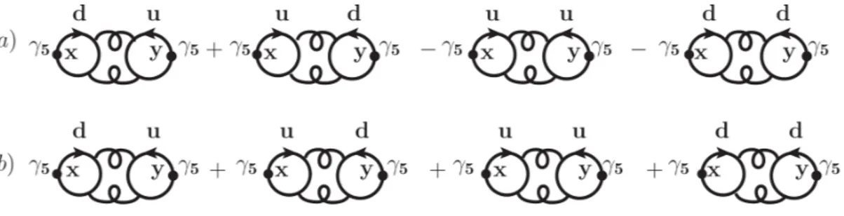
Calculating the fermionic propagator for each degree of freedom and from every space–time point to any other space–time point of the lattice is an enormous task, well beyond the present available computational power. To solve this problem the key observation is that what is really involved in the physical amplitudes is the correlation of the hadronic propagators with a quark-antiquark loop or the correlation between quark-antiquark loop. So the interesting object is the trace of the fermionic propagator over all its degree of freedom. This means that one can profit of stochastic techniques which, focusing their attention to the trace of the fermionic propagator instead of the propagator itself, try to evaluate it with approximate methodologies. We have used as lattice testing observables for these stochastic techniques the 2–point functions of the η′ and of the π0, which involve such a trace.
The present techniques available for calculating the fermionic bubble are two: the dilution method of [13] and the direct method of [14]. After a detailed study of these techniques, we have worked out an hybrid method, which combine what we think are the best virtues of the two methods and which we have called spin–direct method. We will also show a third method [15], the twisted method, which can be employed only using twisted mass fermions and which is less general with respect to the one of [13] and [14] (and to our hybrid method too), but is particularly fast and effective in the case of η′ correlation.
In the η′case, the authors of [16] have succeeded to extract a signal, using the twisted
method, and were able to calculate the η′mass; although they employed some, so–called, variance reduction methods, these techniques are specific of the zero momentum two– points function characteristic of the η′ case. It is clear that such a trick can only be
used when doing spectroscopy while, on the other hand, we want to apply our methods to the neutron EDM calculation and so we can not profit of their variance reduction tricks and we will need to investigate further on a method well suited for the topology calculation characteristic of the EDM.
Analysis and physical results
All our calculations will be carried out at the ApeNext supercomputing center of INFN in Rome using a computational power of few TeraFlop.
Using the correlation functions calculated by the ETM collaboration, we have ex-tract the semileptonic kaon decays form factors at different values of the quark masses simulated on the lattice. We have used the method of the so–called double ratios out-lined in [17; 18; 19] which allows one to gain a high statistical precision in the form factors calculation.
For the K → πlνlwe have used two different strategies for the extrapolation/interpolation
at the physical point: we have exploited quadratic splines to interpolate in the kaon mass, while following the works [19; 20] we have used the SU (2) limit of the SU (3) Gasser and Leutwyler ChPT formulae [21; 22] for reaching the physical point in the pion mass.
Our strategy will be to perform a multi–combined fit of the q2–shape, Mπ and a
dependence of the form factors, using also the constraint given by the Callan-Treiman theorem to further reduce the number of the low–energy constants. In this way we are able give an estimate for the following physical quantities
f+(0) = 0.9610(30)(28),
fK
fπ
= 1.189(8), VKl3
us = 0.2250(14), VusKl2 = 0.2258(16),
where the first error is statistical while the second, where available, is systematic. Our results are in very good agreement with the non-lattice ones obtained from the FLAVIANET collaboration [23] and from the lattice ones by Nf = 2 + 1 simulations of
the RBC/UKQCD collaboration; also the compatibility of our form factor’s q2 shape
with the one obtained by a dispersive fit, based on the form factor parametrization of
[24], to the experimental data from KLOE, KTeV, NA48 (without muons branching
ratios) and ISTRA+ performed by the authors of [23] is good as well.
As far as the use of the stochastic technique to evaluate the disconnected fermionic diagrams is concerned, our main conclusion is that the spin direct method is the most general and promising one. However, since a quite large number of stochastic sources is needed to get a statistically significant signal in the case of the fermionic bubbles, the application of such a method to the more interesting cases related to the neutron
EDM, or to other quantities of phenomenological interest, is possible only on super computers at the PetaFlop scale which will be available in the next future.
Thesis Plan
The first chapter will start introducing some basic notions about flavour physics. We will recall the basis of the Standard Model paying a particular attention to the CKM flavour mixing matrix. We will illustrate some of its related theoretical features and the (phenomenological) determination of its matrix elements. We will then move to leptonic and semileptonic kaon decays, introducing the semileptonic form factors, which are the subject of the present work, ending the chapter introducing weak and strong CP violation, with the latter which is responsible of the neutron electric dipole dipole moment generation.
The second chapter will be dedicated to the introduction of the calculation technique employed in this work: lattice QCD. After a general introduction we will present the Twisted Mass action used by the ETMC and we will also discuss a particular choice for the boundary conditions used in our lattice simulations, the so–called twisted boundary condition.
Chapter three will explain in details the methods which we will employ in our anal-ysis of the form factors as well as the stochastic techniques which are good candidates to be used in a future calculation of the neutron EDM.
In chapter four we will present the results of this work. We will start introduc-ing some basic information about the ETMC simulation which we have analyzed and then we will discuss statistical and systematic error analysis, present our form factor’s analysis strategy and give our final physical results followed by a final discussion of the present status of our stochastic techniques.
Flavour Physics
1.1
The Standard Model
The standard model of electroweak and strong interaction is a Gauge theory invari-ant under the symmetry group SU (3)C ⊗ SU(2)L⊗ U(1)Y; more specifically, it is a
quantum field theory (QFT) with the additional request of invariance under a contin-uous and local1 transformation group.
SU (3)C is the group associated to the so-called color symmetry, on which is based
the present description of the theory of the strong interaction, the quantum chromo-dynamics (QCD). Modern quantum field theories are described as carried by a medi-ator, mathematically represented as a gauge field, which is responsible for the force propagation and interaction and which is called gluon for QCD and represented as Ga, (a = 1, . . . , 8). We will describe QCD and his mathematical formalization in de-tails in chapter 2. The group SU (2)L⊗ U(1)Y is the correct one for describing the
electromagnetic and weak coupling interactions involving gauge (W±, Z0, γ) and mat-ter fields [1]. The electroweak theory is an example of what is called a ”chiral” theory, i.e. a theory in which the left-handed and right-handed components of the fermionic field undergoes different transformation properties; this is what is meant by the letter L which suggests that the interactions described by SU (2)L gauge group involve only
the left-handed components.
Let us point out that, instead, Y labels the weak hypercharge group U (1)Y while with
U (1)Qwe will indicate the quantum electrodynamics (QED) gauge group, whose
ator, the electric charge Q, is related to Y and to the third component of weak isospin by Q = T3+ Y /2. It is clear that being Y a function of the SU (2)Lgenerator, also the
hypercharge group will exibit a chiral character.
Let us now go to discuss some aspects of the model which are particularly relevant for what we will say in the rest of the work.
The gauge invariance request for the interaction is of crucial relevance in building the Standard Model because it provides precise relations between the couplings of the theory and these relations are experimentally confirmed with a high degree of precision; once said that, it is important to remember that for a model with unbroken gauge sym-metry the vector bosons must be massless: an explicit mass term would not be gauge invariant. However the masses of the electroweak gauge bosons W±and Z0 have been
experimentally determined to be different from zero (while photons remain massless1).
The solution to this picture was found in the spontaneous symmetry breaking mecha-nism. With the word spontaneous one mean that a theory, symmetric under a certain group of transformations and with a degenerate vacuum state (think about a potential with a certain number of minima), turns out to be realized selecting a particular vac-uum state among the several possible ones, breaking in that way the formal invariance of the theory. In this framework one has a picture in which the symmetry group is respected by the interaction terms but it is not shared by the vacuum state.
At a somehow practical level, the spontaneous breaking of the electroweak symmetry group is obtained adding an appropriate scalar fields multiplet of SU (2)L ⊗ U(1)Y,
with vacuum expectation value (VEV) different from zero, and which makes possible the achievement of the following breaking path
SU (3)C ⊗ SU(2)L⊗ U(1)Y → SU(3)C ⊗ U(1)Q. (1.1)
What is important to underline is that building a gauge invariant QFT including spontaneous symmetry breaking permits to generate mass terms, proportional to the scalar multiplet vacuum expectation value, for those gauge bosons associated to the broken symmetries (the so called Higgs mechanism [25; 26; 27; 28]). In other words, the spontaneous breaking of the symmetries associated to the W±, Z0 (i.e. SU (2)
L
1This, in turn, imply that because of the weak interaction has a massive mediator, its range is finite in contrast with the electromagnetic interaction which has an infinite range.
and U (1)Y) allows one to keep all the gauge couplings relations but also to generate a
mass term for the electroweak gauge bosons, while leaving SU (3)C ⊗ U(1)Q unbroken
guaranties that the gluon and the photon remain massless.
What has been described up to here can be formalized and summarized writing down the Standard Model lagrangian
LSM = LSU (3)
C+ LSU (2)L⊗U (1)Y + LHiggs, (1.2)
composed of three gauge invariant terms, the first two of them being
LSU (N ) = −1 4F
a
µνFaµν+ i ¯ψγµDµψ . (1.3)
It is a Yang-Mills lagrangian [29] plus a fermionic matter field term. In (1.3) we have indicated with Fa
µν the field strength tensor associated with the Aaµgauge field
Fµνa = ∂. µAaν− ∂νAaµ− gfabcAbµAcν, (1.4)
with ψ a fermionic field which transforms as in the fundamental gauge group represen-tation and with Dµthe covariant derivative, defined as
Dµ= (∂. µ+ igAaµTa) , (1.5)
which, in turn, is composed of a kinetic term for the fermionic field and an interaction term between fermionic and gauge fields.
In the electroweak sector of the theory, the already mentioned fermionic fields are organized in a particular way: left-handed components (in the interaction eigenstates basis) are grouped in SU (2)L doublets
EL1 = µ νe e− ¶ L , EL2 = µ νµ µ− ¶ L , EL3 = µ ντ τ− ¶ L ; Q1L= µ u d′ ¶ L , Q2L= µ c s′ ¶ L , Q3L= µ t b′ ¶ L ; (1.6)
while the right-handed components of quark fields and of the three massive leptons (neutrinos are assumed to be massless in the framework of the Standard Model) are SU (2)L singlets. The choice for the fermionic fields to transform according to this
peculiar representation is motivated by the experimental observation that only the left-handed components of the fermion fields have a role in a weak interaction.
The “chirality feature” of the electroweak interaction forbid the presence of mass terms in the lagrangian not only for gauge bosons, but also for fermions, as can be easily seen from the behavior of a fermionic mass term under a generic gauge group transformation: Lm = m¡ ¯fLfR+ ¯fRfL¢→ L′ m = m ³ ¯ fLUL†URfR+ ¯fRUR†ULfL ´ 6= Lm, (1.7)
with UL 6= UR. However, it has been shown that, in a gauge invariant QFT, it is
possible to obtain mass terms for fermions, once again, using the VEV of the Higgs scalar doublet.
The electroweak interaction lagrangian between matter and gauge fields emerge con-sidering non-kinetic terms in the covariant derivatives, which can be of two kinds:
LEW
int = LCC + LN C , (1.8)
charged currents couplings to W±bosons and neutral currents one to γ and Z0 bosons.
In particular one finds that charged currents interactions are described by
LCC = g 2√2 ³ Jµ†Wµ+ Wµ†Jµ´ , (1.9) with Jµ† = X i=1,3 ¯ uLi γµdiL+ ¯lLiγµνLi , (1.10)
where we have indicated with i the family index for both lepton and quark fields. In view of the fact that we are going to deal with semileptonic meson decays, for which |∆Q| = 1, we are interested in the very (1.9) term of the Standard Model lagrangian.
We remember, for the sake of completeness, that for neutral currents interactions one has LN C = −eJµ emAµ+ g 2 cos θW JZµZµ, (1.11) where Jemµ =PfQff γ¯ µf, JZµ=Pff γ¯ µ(vf − afγ5) f, (1.12) with vf = T3f − 2Qfsin2θW , af = T3f. (1.13)
In these expressions Qfand T3f represents, respectively, the electric charge and the third
components of weak isospin (different from zero only for left-handed fermions); we have also indicated with g and e the SU (2)L and U (1)Q coupling constants, respectively,
and with θW the weak1 mixing angle between the unphysical SU (2)L⊗ U(1)Y gauge
bosons W3 and B and the physical ones Z0 and γ. In table 1.1 we have collected all
the electroweak quantum numbers for the different fermions. νl
L l−L l−R uL dL uR dR
Q 0 -1 -1 2/3 -1/3 2/3 -1/3
T3 1/2 -1/2 0 1/2 -1/2 0 0
Y -1 -1 -2 1/3 1/3 4/3 -2/3
Table 1.1: Electroweak quantum numbers - for leptons and quarks. We have in-dicated with Q the electric charge, T3 the third component of weak isospin and with
Q = T3+ Y /2 the weak hypercharge.
Finally, we can describe the so called Higgs sector of the Standard Model lagrangian
LHiggs= |Dφ|2− V (φ, φ†) + LY (1.14)
1The angle θ
whose expression is determined only by the request of being the most general gauge invariant renormalizable lagrangian for a complex scalar field, φ, which is an SU (2)L
doublet: φ = µ φ+ φ0 ¶ . (1.15)
The potential V (φ, φ†) is invariant under a SU (2)
L⊗U(1)Y transformation and, because
of the renormalizabily constraint, it contains up to quartic terms in φ:
V (φ, φ†) = −µ2φ†φ +1 2λ(φ
†φ)2 , (1.16)
with λ > 0. In this framework, spontaneous symmetry breaking happens if the potential minimum, which represents the classical version of the quantum vacuum state, occurs for values of the φ field which are different from zero; from the shape of the potential V (φ, φ†) it is easy to see that this will happen if µ2 > 0. Assuming that this is the
case, let us choose as the VEV φ value
h0| φ(x) |0i = µ 0 v ¶ 6= 0 . (1.17)
The field component with VEV different from zero is the neutral one and this imply that the vacuum has trivial transformation properties under U (1)Qand that this group
will still be a symmetry of theory after the spontaneous breaking. It is possible to make more explicit the particle spectrum of the theory, taking advantage of the arbitrariness of the gauge choice. In particular one can parametrize the Higgs doublet as a VEV part plus a part which measure how much the field is different from v :
φ(x) = U (x)√1 2 µ 0 v + h(x) ¶ , (1.18)
where h(x) is a real field whose VEV is zero and U (x) ∈ (SU(2) ⊗ U(1)Y); U (x) can
be simplified making the inverse gauge transformation U (x)−1 which brings us in the so called unitary gauge. In this gauge the field φ becomes
φ(x) = √1 2 µ 0 v + h(x) ¶ , (1.19)
and the particle content (and spectrum) of the theory is already manifest at a lagrangian level: the goldstone boson degrees of freedom appear only as the longitudinal gauge boson degrees of freedom and we are left only with physical particles1.
Let’s now describe the Standard Model lagrangian term which is responsible for the fermionic masses: LY; assuming there are no right handed neutrinos, this term is the
most general one describing the coupling of the Higgs doublet with fermionic fields, again constrained only by gauge invariance and renormalizability requests:
LY = −λij
l E¯LiφejR− λ ij
dQ¯iLφdjR− λuijQ¯iLφu¯ jR+ h.c. , (1.20)
where the field ¯φ is defined as ¯φα = ǫαβφ∗
β, with ǫ the SU (2)L antisymmetric tensor
and α, β the relative (isospin) indices. The complex-valued matrices λl, λu and λd are
not necessarily hermitian nor symmetric and i,j = 1, 2, 3 are generation indices; unless one don’t ask for a flavour conserving symmetry, interactions with Higgs field will be flavour changing.
It is always possible to diagonalize λl by means of a redefinition of the leptonic fields: a
generic, complex valued matrix can always be rewritten in terms of a diagonal matrix Dl = diag(˜λe, ˜λµ˜λτ) with positive eigenvalues and two unitary matrices
λl= UlDlWl† (1.21)
in order that, rescaling the fields
ELi → UlijELj , eiR→ WlijejR, (1.22)
the leptonic part of the Yukawa term becomes
1We want to stress the fact that, although the unitary gauge is a good choice to analyze the particle content and mass spectrum of the theory, it is less well suited for studying quantum corrections to the classical theory and, to this end, different gauges should be chosen.
− ˜λeE¯LeφeR− ˜λµE¯LµφµR− ˜λτE¯τLφτR. (1.23)
Both the weak isospin doublet components undergoes the same Ul transformation and
this imply that the matrices Ul and Wl cancels everywhere in the theory1 and the
phenomenological consequence of this cancellation is that one has exact conservation of the leptonic number for each generation and no CP violation, as has been precisely tested in the experiments [30]. Inserting the expression (1.19) for the φ field in the unitary gauge one has, for a generic lepton li
L(l) Y = −mil¯lili µ 1 +h v ¶ , mil=. √1 2D ii l v . (1.24)
The spontaneous breaking of gauge symmetry generates an interaction term with the Higgs field h(x) as well as a mass term for leptons.
Next section will be dedicated to the analogous mechanism for the quark sector.
1.2
Cabibbo-Kobayashi-Maskawa matrix
In this section we will broaden the Standard Model flavour sector overview, describ-ing the flavour mixdescrib-ing matrix, also known as Cabibbo-Kobayashi-Maskawa matrix. What we are going to show is that weak interactions, in the quark sector, are not flavour diagonal in the mass eigenstates basis and the mixing matrix contains all the information we need to know about the relative weights for quark decays in their weak isospin partner of each generation.
1.2.1 Definition & parametrization
Let us analyze the Yukawa coupling between the Higgs doublet and the quark fields. First of all it is important to underline that the effect of the CP discrete symmetry is equivalent to the substitution
λijd → (λijd)∗, λiju → (λiju)∗ , (1.25)
and so CP is a symmetry only if the matrices λij are real.
Following what has been done in the previous section for the leptonic sector we are going to perform chiral transformations of the kind
λu= UuDuWu† and λd= UdDdWd†, (1.26)
where the matrices D are diagonal with positive eigenvalues, while U and W are unitary matrices; rescaling right-handed fields with
uiR→ WuijujR and diR→ WdijdjR, (1.27)
one is able to simplify the W matrices present in the Yukawa coupling lagrangian. The same can be done in covariant derivatives leaving unchanged right-handed quarks kinetic terms. Similarly, on left-handed quark we can make the transformation
uiL→ UuijujL, diL→ UdijdjL, (1.28)
and we are able to simplify the U matrices from the Yukawa coupling lagrangian which become L(q) Y = −midd¯iLdiR µ 1 +h v ¶ − miuu¯iLuiR µ 1 +h v ¶ , (1.29) where mu,d =. 1 √ 2D ii u,dv . (1.30)
What is now different is that we are analyzing left-handed field, and left-handed fields participate in the SU (2)L interaction, which is the flavour mixing one, and it makes
necessary studying how does it changes, if it does, the rest of the lagrangian under the transformations (1.28).
First of all, U matrices cancel out in kinetic terms and in the interaction ones with gluonic fields because they are both flavour diagonal; the interaction terms with the
electromagnetic (Aµ) and the neutral weak mediator (Z0) fields remain unchanged too,
considered that they don’t mix up fields with down fields. On the contrary, charged currents transforms as Jµ† = √1 2u¯ i LγµdiL→ 1 √ 2u¯ i LγµVCKMij d j L, (1.31)
expression in which we have defined the Cabibbo-Kobayashi-Maskawa (CKM) [2; 3] flavour mixing matrix as
VCKM = U. u†Ud (1.32)
and it connects the interaction eigenstates (d′, s′, b′) with the mass eigenstates (d, s, b):
d′ s′ b′ = Vud Vus Vub Vcd Vcs Vcb Vtd Vts Vtb d s b . (1.33)
From this point of view it is clear that mass eigenstate are different from the interaction ones and that charged current interaction mix different flavours with weight Vij in the
mass eigenstates basis. It is worthwhile to underline that within the Standard Model
the only flavour changing mechanism is represented by this matrix and that VCKM
unitarity guarantees that there are no flavour changing neutral currents (FCNC) to first order of perturbation theory; moreover the suppression of FCNC at higher orders, the so called GIM mechanism [31], is a consequence of VCKM and well represents what
has been experimentally observed in nature.
The CKM matrix, in the case of three quark generations, is a 3 × 3 unitary complex matrix which depends on nine real numbers1. Exploiting the quark fields phase redefi-nition freedom, it can be easily shown that VCKM depends only on 4 real parameters,
three angles and one phase, which, together with fermion masses, constitute the free parameters relative to the flavour sector of the Standard Model.
Once the number of the independent physical parameters of the matrix is known, one can introduce a set of different parametrization for that matrix depending on what
1
one has to study. The most natural choice is the one presented in [32] which writes the matrix as a product of three different rotations
VCKM = 1 0 0 0 c23 s23 0 −s23 c23 c13 0 s13e−iδ 0 1 0 −s13eiδ 0 c13 c12 s12 0 −s12 c12 0 0 0 1 , (1.34) which leads to VCKM = c12c13 s12c13 s13e−iδ −s12c23− c12c23s13eiδ c12c23− s12s23s13eiδ s23c13 s12s23− c12c23s13eiδ −c12s23− s12c23s13eiδ c13c23 , (1.35)
where sij = sin θij, cij = cos θij (and θ12is the Cabibbo angle) and δ is the phase. The
angles θij can be chosen in the first quadrant in order that sij and cij ≥ 0. What is
important to underline is that if δ = 0 the matrix VCKM becomes real and one has
no CP violation in the quark sector too. Another interesting feature of the matrix is that the δ phase is present in the Standard Model because the quark are organized in three generations. In the old Cabibbo version of the theory, which involved only two generations (u, d) and (c, s), the mixing matrix was a real rotation (in flavour space) and there was no room for CP violation. Moreover in order for CP violation to happen, it is necessary for up - like (as well as down - like) quark masses to be different because if it is not the case, by means of suitable unitary transformation, one could redefine quark fields in order to simplify the CP violating phase. It can be shown that the necessary condition for having CP violation is
(m2t − m2c)(m2t− m2u)(m2u− m2c)(m2b − m2s)(m2b− md2)(m2d− m2s) × JCP 6= 0 (1.36)
where we have introduced the Jarlskog parameter [33;34]
JCP = |Im(V. ijVklVil∗Vjk∗)| , (i 6= k, j 6= l) , (1.37)
which can be thought as a quantitative way of measuring how much CP symmetry is violated. JCP is not dependent on quark fields phase conventions and VCKM unitarity
imply that all the allowed i,j,k,l combinations will give the same quantity. Using Maiani parametrization (1.35) one has
JCP = s12s13s23c12c23c213sin δ ; (1.38)
experimentally it has been measured JCP ≃ O(10−5).
As one can clearly see from (1.36) the CP violation root can be traced back to the quark mass hierarchy problem; as already said, fermion masses are free parameters in the Standard Model. The weak interaction mixes flavors according to a specific hierarchy: the diagonal elements of the matrix (1.33) describe transition within the same generation and are bigger (∼ O(1)) than off diagonal elements (∼ O(10−1) to ∼
O(10−3)), which, on the other hand, represent transitions between generations, for which experimentally one has s13≪ s23 ≪ s12 ≪ 1. This has been pictorially represented in
figure1.1where transitions within the same generation are represented with bold black lines, while transitions between different generations are represented with dashed and dotted lines of different colors.
Figure 1.1: Flavour mixing hierarchy - It is shown the hierarchy of charged currents flavour mixing transition; picture taken from [35](Fleisher’s lecture).
It is convenient to exhibit this hierarchy setting
s12= λ ,. s23= Aλ. 2, s13e−iδ = Aλ. 3(ρ.iη) , (1.39)
and substituting them in (1.35) one obtains the CKM matrix parametrization in terms of (λ, A, ρ, η) proposed by Wolfenstein in [36]. Expanding the matrix elements in powers of λ, neglecting terms O(λ4) one has
VCKM = 1 −λ22 λ Aλ3(ρ − iη) −λ 1 −λ22 Aλ2
Aλ3(1 − ρ − iη) −Aλ2 1
+ O(λ4) . (1.40)
With this variables the Jarlskog invariant becomes
JCP = Aλ6η , (1.41)
and the measure of CP violation, analogous to δ of the standard parametrization, is η (as can be seen from (1.40), if η is zero elements (VCKM)13 and (VCKM)31 become real
and no CP violation is possible).
Other important information can be extracted from CKM matrix performing the so called unitarity triangle analysis. This kind of analysis is based on the unitarity of VCKM which can be expressed as
VCKM† VCKM = VCKMVCKM† = 1 , (1.42)
and, if expressed element by element, it consists of nine relations, six of orthogonality and three of normalization. The former can be represented as six triangles in a complex plane, all having the same area A∆ = JCP/2; using Wolfenstein’s parametrization
for CKM elements it can be realized that only the triangle’s sides coming from the orthogonality of first and third row and first and third column are of the same order of magnitude (O(λ3)); they are
VudVub∗ + VcdVcb∗ + VtdVtb∗= 0 (1.43)
VudVtd∗ + VusVts∗+ VubVtb∗= 0 (1.44)
for other triangles one has a side that is smaller than the other roughly by a factor O(λ2) o O(λ4). Actually relations (1.43) and (1.44) are equivalent at order O(λ3) and one can write them as
and so at this order one has only one independent triangle and we will choose in the following the usual (1.43) also known as unitary triangle of CKM matrix.
It can be shown [37] that performing in (1.45) the substitution (ρ, η) → (¯ρ, ¯η), with the barred parameters defined by
ρ − iη = √ρ − i¯η¯
1 − λ2 , (1.46)
one can obtain a unitarity relation valid up to order O(λ7)
[(¯ρ + i¯η) + (−1) + (1 − ¯ρ − i¯η)] Aλ3+ O(λ7) = 0 (1.47) and the associated unitary triangle is shown in fig. 1.2
Figure 1.2: Unitary triangle - It is shown the unitary triangle related to (1.47); picture taken from [30](PDG 2008)
where sides and angles are defined as follows
α= φ. 2 = arg. µ −VtdV ∗ tb VudVub∗ ¶ , (1.48) β = φ. 1 = arg. µ −VcdV ∗ cb VtdVtb∗ ¶ , (1.49) γ = φ. 3 = arg. µ −VudV ∗ ub VcdVcb∗ ¶ , (1.50) Rb =. |Vud V∗ ub| |VcdVcb∗| ≃ µ 1 −λ 2 2 ¶ 1 λ ¯ ¯ ¯ ¯ Vub Vcb ¯ ¯ ¯ ¯ , (1.51) Rt=. |Vtd V∗ tb| |VcdVcb∗| ≃ 1 λ ¯ ¯ ¯ ¯ Vtd Vcb ¯ ¯ ¯ ¯ . (1.52)
1.2.2 Experimental determination
Assuming the Standard Model as a complete model, the “experimental” measure of VCKM elements should verify its unitarity. Deviation from that expected unitarity
would unambiguously indicate the presence of physics beyond the Standard Model; hence it is of crucial relevance to perform as precise as possible measures to increase our knowledge of the Standard Model and of potential new physics. For instance, in view of the upcoming measures which will be performed at the LHC, it will be very important to know the flavour sector parameters as well as possible in order to better understand a possible discovery of new particles or new physics.
Within the Standard Model, all flavour violating processes, both CP violating and con-serving ones, are ruled by CKM matrix and, as a consequence, can be described by means of four parameters (three angles and one phase or, using Wolfenstein parametriza-tion, A,λ,ρ and η); this means that the large variety of flavour physics phenomena which are nowadays measurable (i.e. semileptonic decays, CP asymmetries, neutral mesons mixing, rare decays and so on) are all strongly connected and the unitary triangle is an optimal tool for studying these correlations. More specifically, thanks to the B-factories measures as well as to D and K decays measurements and moreover to the higher lat-tice QCD accuracy in providing theoretical inputs, it is possible to overconstrain the unitary triangle. This means that, eventually, it is possible to correctly test the CKM mechanism within the Standard Model and to set limits on the possible new physics contributes. Let us now briefly remind, according to the 2008 edition of the Review of particle physics [30], the physical processes from which it is possible to measure the CKM elements.
Starting from Vud, the most precise determination of the module of this element
comes from superallowed JP = 0+ → JP = 0+ nuclear beta decays, which are pure
vector transitions and are free from nuclear structure uncertainties. This yields
|Vud| = 0.97418 ± 0.00027 . (1.53)
It is also possible to measure this matrix element using neutrino lifetimes or from the branching ratio for the process π+ → π0e+ν and both give results consistent with (1.53) but with a slightly bigger error.
Without going into details, as these are going to be the subject of next section, let’s mention that |Vus| can be extracted from KL0 → πeν decays using the form factor
extracted from lattice QCD as theoretical input, and it yields [23]1
|Vus| = 0.2254 ± 0.0013 . (1.54)
Other possible determination of |Vus| involve leptonic kaon decays, hyperon decays and
τ decays. From the first, one can extract a value of [23]
|Vus| = 0.2312 ± 0.0013 , (1.55)
using again the lattice QCD input of the ratio of the pion and kaon decay constants togheter with the knowledge of |Vud|.
What is important to underline is that the quoted errors in (1.54) and (1.55) are
dominated by the uncertainty on the LQCD hadronic quantity used to obtain Vus
matrix element from the experimental data (respectively, the form factor and the ratio of decay constants). It is clear that a precise determination of these quantities on the lattice is needed in order to improve more and match the experimental precision.
For extracting |Vcd| one can use a measure based on neutrino and antineutrino
interaction. The measure of the difference of the ratio of double muon to single muon production is proportional to the charm cross section off valence d-quarks and therefore to |Vcd|2. Using a suitable average one can obtain
|Vcd| = 0.230 ± 0.011 . (1.56)
A direct determination of |Vcs| is possible from semileptonic D or leptonic Ds
de-cays, using again lattice QCD calculations as input for D form factors and Ds decay
constants. Here the state of the art is similar to the |Vus| one, in which the error on
the CKM element is completely dominated from the theoretical one. From averaged leptonic and semileptonic determinations ref. [30] quotes
1The value presented here is slightly different from the one in [30] because of the updated value recently presented in [23].
|Vcs| = 1.04 ± 0.06 . (1.57)
The |Vcb| matrix element can be determined from exclusive and inclusive
semilep-tonic decays of B mesons to charm. The inclusive determination use the semilepsemilep-tonic decay rate measurement, together with the leptonic energy and the hadronic invariant mass. Exclusive determinations are based on semileptonic B decays to D and D∗. In
the limit mb,c ≫ ΛQCD the form factors can be calculated using heavy-quark effective
theory (HQET) and Vcbcan be obtained from and extrapolation guided by this effective
theory. The exclusive determination is less precise than the inclusive one, because the theoretical uncertainty in the form factors and the experimental uncertainty in the rate near the physical point are about 3%. A suitable combination of the two results yields
|Vcb| = (41.2 ± 1.1) × 10−3. (1.58)
The determination of |Vub| from inclusive B → Xul¯ν decay suffers from large
B → Xcl¯ν backgrounds. In most regions of phase space where the charm background
is kinematically forbidden, hadronic physics enters via unknown nonperturbative func-tions, called shape functions. These functions must be measured in different processes, such as B → Xsγ, and then applied to several spectra in B → Xul¯ν. There are also
other methods in which one applies phase space methods to reduce the number of shape functions presents in the rate; another alternative approach is to extend the measure-ment deeper into the B → Xcl¯ν region to reduce the theoretical uncertainties. Vub
can also be extracted from an exclusive channel, assuming the form factors are known. Form factors can be measured or calculated using LQCD (in the kinematic region of q2 > 16 GeV2) or light cone QCD sum rules for q2 < 14 GeV2 and all yield similar results when used in Vub calculation. The theoretical uncertainties in extracting |Vub|
from inclusive and exclusive decays are different; a combination of the determinations is quoted as
which is dominated by the inclusive measurement.
The CKM elements |Vtd| and |Vts| cannot be measured from tree-level decays of
the top quark, so one has to rely on determinations from B − ¯B oscillations mediated by box diagrams with top quarks, or loop-mediated rare K and B decays. Theoretical uncertainties in hadronic effects limit again the accuracy of the current determination. These can be reduced by taking ratios of processes, as an example one could quote the quantity ∆md/∆ms, that are equal in the flavour SU (3) limit to determine |Vtd/Vts|.
Without doing so and using unquenched LQCD calculation for the hadronic quantities one finds
|Vtd| = (8.1 ± 0.6) × 10−3, |Vts| = (38.7 ± 2.3) × 10−3. (1.60)
The uncertainties are dominated by LQCD calculations; however if one takes the ratio ∆md/∆ms, which in turn involve the ratio of the hadronic quantities determined on
the lattice, is able to obtain the more reliable constraint for ¯ ¯ ¯ ¯ Vtd Vts ¯ ¯ ¯ ¯ = 0.209 ± 0.001stat± 0.006sys. (1.61)
A complementary determination for the ratio of these matrix elements is possible from the ratio of B → ργ and K∗γ rates, which gives |V
td/Vts| = 0.21 ± 0.04 while for the
product |VtdVts∗| one can use the rare decay K+→ π+ν ¯ν but experimentally only three
events has been observed and much more data are needed for a precision measurement. Finally the determination of Vtb from top decays uses the ratio of the branching
fractions R = B(t → W b)/B(t → W q) = |Vtb|2, with q = b, s, d. Experimental measures
give for these quantities |Vtb| > 0.78 and |Vtb| > 0.89. Direct determination of Vtb
without assuming unitarity is possible from single top quark production cross section. In this way it is possible to set the limit
|Vtb| > 0.74 . (1.62)
Also, one can constrain |Vtb| from electroweak data and the result, mostly driven by
|Vtb| = 0.77+0.18−0.24. (1.63)
To summarize we can write, restricting our attention to the direct measure of the module of CKM elements VCKMexp = 0.97418 ± 0.00027 0.2254 ± 0.0013 (3.93 ± 0.36) × 10 −3 0.230 ± 0.011 1.04 ± 0.06 (41.2 ± 1.1) × 10−3 (8.1 ± 0.6) × 10−3 (38.7 ± 2.3) × 10−3 0.77+0.18−0.24 . (1.64) To proceed with unitary triangle angles, measurement of CP violation effects in neutral B mesons decays provide a determination of sin 2β. Word average quotes
sin 2β = 0.681 ± 0.025 , (1.65)
while the results for α, coming from time dependent CP asymmetries in b → u¯ud
dominated decays, and for γ, coming mainly from B±→ DK± are
α =¡88+6−5¢◦ (1.66)
γ =¡77+30−32¢◦ (1.67)
Another way for extracting values of the CKM matrix elements which are more accurate with respect to ones in (1.64), is to perform a fit [38; 39] of all the latest available measures imposing all the Standard Model constraints. The results obtained in that way reported in [30] are
VCKMf it = 0.97419 ± 0.00022 0.2257 ± 0.0010 (3.59 ± 0.16) × 10 −3 0.2256 ± 0.0010 0.97344 ± 0.00023 ¡41.5+1.0−1.1¢× 10−3 ¡ 8.74+0.26−0.37¢× 10−3 (40.7 ± 1) × 10−3 0.999133+0.000044−0.000043 , (1.68) while Wolfenstein’s parameters are
λ = 0.2257+9−10, (1.69) A = 0.814+21−22, (1.70) ¯ ρ = 0.135+31−16, (1.71) ¯ η = 0.349+15−17. (1.72)
Let us conclude this section underlining again the importance of the lattice QCD calculation of meson decay form factors. First of all, it is important because the form factors are needed both in the theoretical as well as on the experimental side, to extract from what one experimentally measures the CKM matrix element; moreover it is important to give a precise estimate of the form factors because in most of the processes the experimental precision is so high that, at the end of the day, all the systematic error comes from the theoretical side , and in the present case, from the lattice QCD uncertainty on the hadronic quantity.
A special mention for the semileptonic K decay is in order, as the experimental precision is so high, of the order of 0.2%, that the form factor at zero momentum must be determined with a precision better that the percent level. This is feasible with a technique which will be shown in chapter3.
1.3
Leptonic and semileptonic meson decays
Within the Standard Model, as we have already mentioned, leptonic and semilep-tonic meson decays can be used to obtain accurate determinations of the magnitude of the CKM elements and, in particular, semileptonic Kaon decays gives us the best determination of the magnitude of the Vus element. A general feature of standard
anal-ysis is that for extracting these elements from decay widths one need precise estimates about the relevant hadronic quantities involved in the process; to be more specific, it is necessary to know decay constants and semileptonic form factors, as a function of the transfer momentum, in a very precise fashion.
At the energy scale characteristic of an hadronic decay process, strong interaction can-not be treated by means of perturbative methods because αs&1. This means that the
hadronic quantities involved in the decay widths must be estimated using non pertur-bative techniques, and in particular a lattice QCD calculation of the kaon semileptonic decay constant and form factor will be presented in chapter 4 and will be one of the main goals of this work.
Within the quark model mesons are represented as quark-antiquark bound states ¯
qq′ with the two quarks, known as valence quarks, which can have different flavour. Writing the orbital angular momentum of the system as l, the meson parity P can be calculated as P = (−1)l+1; total angular momentum, J, is as usual made up of orbital
angular momentum and spin angular momentum and will take values in the interval |l − s| < J < |l + s|, where s = 0, 1 if the quark’s spins are antiparallel or parallel, re-spectively. In real word, however, mesons, and more generally hadrons, are much more complicated objects and valence quarks are responsible only for the particle’s quan-tum numbers. An hadron is composed of an infinite number of quarks, antiquarks and virtual gluons, known as Dirac sea, which gives null contribution to the hadron quan-tum numbers. In this framework, hadron decays can be seen as their valence quarks weak decays. The matrix element spin structure is particularly simple for pseudoscalar mesons (JP = 0−) and their description can be done in terms of few free parameters.
We will distinguish between two meson’s classes: light mesons, composed of two light quarks q, q′ = u, d, s and heavy-light mesons, built up by one heavy quark Q = c, b and
one light quark q = u, d, s; moreover we will also restrict ourselves to that decays which are first order in the weak coupling, focusing our attention to the flavour changing processes which, as we have already seen in the previous section, at tree level come only from charged current interactions in the Standard Model because of unitarity of the CKM matrix.
Let us now introduce a new element which will be useful in the following sections: Fermi effective theory of weak interaction. Semileptonic decays are processes in which W±
bosons (but this is true also for Z0 boson) have masses which are large in comparison with q, the typical transfer momentum involved; in practice, this means that terms of order O(q2/MW2 ) and higher, can be safely neglected from the physical amplitudes. This is usually referred to as the W± decouples from the theory in the low energy
regime and they end up “integrated out”. The result of this operation is an effective theory, valid at energies E ≪ MW,Z, in which there are no more W± or Z0 and the
non local interaction which were mediated by these bosons are now seen as local four fermions interactions: −igµν q2− M2 W −−−−−→ M2 W≫q2 −igµν M2 W . (1.73)
At a lagrangian level one has
Lef f CC = GF √ 2J † µJµ · 1 + O( q 2 M2 W ) ¸ , (1.74)
where GF is the so called Fermi constant defined in terms of the weak coupling constant g as GF √ 2 . = g 2 8MW2 . (1.75)
As charged weak currents (1.10) describe both quarks and leptons, it follows that the effective lagrangian (1.74) will in turn describe interactions between two lepton currents, which are responsible for processes such as τ or µ leptonic decays, between one lepton current and an hadronic one, which can account for leptonic and semileptonic hadron decays and, in the end, between two hadronic currents which describe non leptonic hadron decays.
1.3.1 Leptonic Kaon decays
Leptonic decays are processes in which the final state is purely leptonic. Among them one could quote
π+→ µ++ νµ
D±s → µ±+ νµ(¯νµ)
B+→ τ++ ντ
and so the prototype, for the case of a negative meson M−, can be represented as
M−→ l−ν¯
l which is related to the underlying quark process q ¯q′ → lνl, as can be seen
in figure 1.3
The decay width for such a process can be written as
Γ(M−→ l−νl) = 1 2M X pol Z |A2|dΩ2 (1.76)
where M is the meson mass, the sum is over the polarization of the final state leptons, A is the Feynman amplitude for the process and dΩ2 is the two body phase space. The
amplitude, at lowest order in the electroweak interaction but to all orders in the strong interaction, can be written as
Figure 1.3: Leptonic decay prototype - Feynman diagram which contribute to a leptonic decay of a general meson M. The hadronic part (left) must be evaluated by means of non perturbative methods.
A(M−→ l−νl) = − GF √ 2V ∗ q′qhl−νl| £ ¯ νlγµ¡1 − γ5¢l¤ £qγ¯ µ¡1 − γ5¢q′¤|M−i ; (1.77)
because of the point-like interaction between the two currents, the amplitude factors out in two parts, one leptonic and one hadronic:
A(M− → l−νl) = − GF √ 2V ∗ udHµLµ (1.78)
where it has been defined
Hµ= h0| ¯qγ. µγ5q′|M−i , (1.79)
Lµ= hl. −ν¯l| ¯lγµ
¡
1 − γ5¢νl|0i . (1.80)
Two remarks are in order. First of all, the vacuum insertion is possible only because (at this order) there are no radiative corrections between the initial and the final state. The second one is that because of in (1.79) the initial and the final states have different parity, only the axial contribute to the amplitude is present. The problem is now shifted to the evaluation of Hµ. Taking into account Lorentz-invariance one knows that expression (1.79) must be parametrized as a vector times a quantity, fM, which
has the dimension of an energy and must be experimentally determined; as the only vector present in the process is the meson momentum pµ, one can write
h0| ¯qγµγ5q′|M−i = −ifMpµ. (1.81)
The parameter fM is called the M meson decay constant and represents the overlap of
the two valence quark and antiquark wave functions.
Evaluating two body phase space and kinematics, the square module of the Feynman amplitude (1.78) and substituting them into eq. (1.76), one obtain the decay width
Γ(M− → l−νl) = G2F 8πf 2 M|Vq′q|2M m2 µ 1 − m 2 M2 ¶2 , (1.82)
where m is the l lepton mass, assuming antineutrinos are massless.
Formula (1.82) is the starting point for the evaluation of the CKM matrix element Vus using leptonic Kaon decays. In particular, what is usually employed is not
expres-sion (1.82) specified for H±= K± alone (the so called K±
l2 decay width), but the ratio
of the K±→ l±ν to π±→ l±ν (called π± l2) [40;41] decay width: ΓKl2 Γπl2 = |Vus| 2 |Vud|2 f2 K f2 π mK ³ 1 − m2l m2 K ´2 mπ ³ 1 − m2l m2 π ´2 (1 + δEM) . (1.83)
where fK and fπ are the kaon and the pion decay constants and δEM denotes the effect
of long distance electromagnetic corrections. Short distance radiative effects are uni-versal and cancel in the ratio. In the approximation of point-like kaons and pions, the long distance electromagnetic corrections depend only on particle masses. The domi-nant uncertainty on δEM comes from terms depending on the hadronic structure. Most
analysis to date make use of the results quoted in ref. [42; 43], which was computed using a model with Breit - Wigner form factors for the low - lying vector resonances. These results give δEM = −0.0070(35) (see [44]). Using chiral perturbation theory
(ChPT)[40;45], it has been shown that to leading non trivial order O(e2p2), the
struc-ture dependent corrections to δEM can be expressed in terms of the electromagnetic
pion mass splitting. With the relative theoretical uncertainty estimated at 25% to account for O(e2p4) effects suppressed by chiral power counting, one obtains
With experimental measurements of the inclusive Kl2 and πl2 decay rates and precise
knowledge of the radiative corrections, eq. (1.83) can be used to obtain the value of the product |Vus/Vud|2× fK2/fπ2, from which one can estimate Vus once estimated the
ratio fK/fπ on the lattice.
1.3.2 Semileptonic Kaon decays
Semileptonic decays are processes in which the final state is composed of leptons and hadrons; among them one can quote
N → N′+ e±+ νe(¯νe) (1.85)
π+→ π0+ e++ νe (1.86)
k+→ π0+ e++ νe (1.87)
D+→ ¯K0+ e++ ¯νe (1.88)
where N is a generic nucleus and N′differs from N by one u → d in the valence content. In each decay the quark underlying process is q → q′′lν
l and the quark q′ participate
only as spectator (see fig. 1.4).
Figure 1.4: Semileptonic decay prototype - Feynman diagram which contribute to the semileptonic decay process M → M′l¯ν
l. The hadronic part (bottom) must be evaluated
by means of non perturbative methods.
In this case the situation is much more complicated, with respect to the leptonic case, because of the composition of the final state (leptons plus an hadron); writing
the initial state meson as M and the final state one as M′, the Feynman amplitude for the process, at lowest order in the electroweak interaction but all orders in the strong interaction, can be written as
A(M → M′lνl) = − GF √ 2V ∗ q′qhM′l−νl| £ ¯ νlγµ ¡ 1 − γ5¢l¤ £qγ¯ µ¡1 − γ5¢q′¤|M−i ; (1.89) however, the amplitude factors out in an hadronic times a leptonic part. This is again because the leptons present in the final state do not strongly interact and moreover because the hadronization process involves only the valence quark of the final state meson. This can be written as
A(M → M′l−νl) = − GF √ 2V ∗ q′qhl−νl| ¯νlγµ ¡ 1 − γ5¢l |0i hM′| ¯qγµ¡1 − γ5¢q′|Mi . (1.90) Limiting our attention to the case in which the JP of the initial state is the same of
the final state one, that is 0− → 0− decays which, by the way, are the subject of the
present work, the hadronic matrix element receive only the vector contribution and we are left with
A(M → M′l−νl) = − GF √ 2V ∗ q′qHµLµ (1.91) where Hµ= hM. ′(k)| ¯qγµq′|M(p)i , (1.92) Lµ= hl¯ν. l| ¯lγµ ¡ 1 − γ5¢νl|0i . (1.93)
Eq. (1.92) tell us that the matrix element transform as a vector and so we can
parametrize it using the only two vectors at our disposal in the process, i.e. the initial state meson momentum p and the final state meson one k, so
hM′(k)| ¯qγµq′|M(p)i = (p + k)µf+(q2) + qµf−(q2) (1.94)
where we have used the independent linear combinations p + k and q = p − k and hadronic effects, which do not follow by symmetry arguments, are described by means
of the form factors f±(q2). f+(q2) is called vector form factor and usually f−(q2) is
traded for the scalar form factor, defined as
f0(q2) = f+(q2) +
q2 M2
f − Mi2
f−(q2) (1.95)
which satisfy the kinematic constraint f0(0) = f+(0) and where Mi(Mf) is the mass of
the meson state M (M′).
Let us specialize to the case, relevant for this work, of the kaon semileptonic decays; these decays are the relevant one for extracting the CKM matrix element Vusand their
prototype is represented by processes such as
K+→ π0+ l++ νl (1.96)
K0→ π++ l−+ ¯νl (1.97)
which are usually called Kl3 decays and in which the underlying quark transition is
s → u + W−. The partial conservation of the vector current (PCVC)
∂µVµa= i ¯ψ · λa 2 , m ¸ ψ , (1.98)
where Vµa= ¯ψγµtaψ is the non singlet vector current, m is the quark mass matrix and ta= λa/2 are the SU (3) generators, can be considered for the s → u transition under exam, obtaining
∂µ(¯uγµs) ∝ (ms− mu) ¯us , (1.99)
where ms(u) is the mass of the s(u) quark; Neglecting SU (3)V flavour breaking effects,
i.e.
δm → 0 ⇒ ∂µVµ= 0 (1.100)
a conserved current and a related conserved charge will exist and it is possible to show that
![Figure 1.2: Unitary triangle - It is shown the unitary triangle related to ( 1.47 ); picture taken from [ 30 ] (PDG 2008)](https://thumb-eu.123doks.com/thumbv2/123dokorg/2833092.4555/33.918.261.573.474.653/figure-unitary-triangle-shown-unitary-triangle-related-picture.webp)