A 2D markerless gait analysis methodology: validation on healthy subjects

(1)

Research Article

A 2D Markerless Gait Analysis Methodology:

Validation on Healthy Subjects

Andrea Castelli,

1,2

Gabriele Paolini,

1,2

Andrea Cereatti,

1,2

and Ugo Della Croce

1,2

1_{Department of Information Engineering, Political Sciences and Communication Sciences, University of Sassari, 07100 Sassari, Italy} 2_{Interuniversity Centre of Bioengineering of the Human Neuromusculoskeletal System, Sassari, Italy}

Correspondence should be addressed to Andrea Cereatti; acereatti@uniss.it Received 9 January 2015; Revised 5 April 2015; Accepted 7 April 2015 Academic Editor: Reinoud Maex

Copyright © 2015 Andrea Castelli et al. This is an open access article distributed under the Creative Commons Attribution License, which permits unrestricted use, distribution, and reproduction in any medium, provided the original work is properly cited. A 2D markerless technique is proposed to perform lower limb sagittal plane kinematic analysis using a single video camera. A subject-specific, multisegmental model of the lower limb was calibrated with the subject in an upright standing position. Ankle socks and underwear garments were used to track the feet and pelvis segments, whereas shank and thigh segments were tracked by means of reference points identified on the model. The method was validated against a marker based clinical gait model. The accuracy of the spatiotemporal parameters estimation was found suitable for clinical use (errors between 1% and 3% of the corresponding true values). Comparison analysis of the kinematics patterns obtained with the two systems revealed high correlation for all the joints(0.82 < 𝑅2 < 0.99). Differences between the joint kinematics estimates ranged from 3.9 deg to 6.1 deg for the hip, from 2.7 deg to 4.4 deg for the knee, and from 3.0 deg to 4.7 deg for the ankle. The proposed technique allows a quantitative assessment of the lower limb motion in the sagittal plane, simplifying the experimental setup and reducing the cost with respect to traditional marker based gait analysis protocols.

1. Introduction

Three-dimensional (3D) marker-based clinical gait analysis is generally recognized to play an important role in the assessment, therapy planning, and evaluation of gait related

disorders [1]. It is performed by attaching physical markers

on the skin of the subject and recording their position via multiple cameras. To date, optoelectronic stereophotogram-metric systems represent the most accurate technology for

the assessment of joint kinematics [2]. While the 3D

char-acterization of motion represents the standard for clinical gait analysis laboratories and research environments, 3D gait analysis remains underused in ambulatory environments due to the costs, time, and technical requirements of this technology.

Multicamera, video-based markerless (ML) systems can represent a promising alternative to 3D marker-based systems

[3–5]. In fact, the use of ML techniques does not require the

application of fixtures on the skin of the patients [1], making

the experimental sessions faster and simpler (e.g., do not

have to worry about markers falling off during the sessions)

[1]. 3D ML motion capture techniques have been extensively

presented in [5–9] for different types of applications,

includ-ing clinical gait analysis and biomechanics. However, 3D ML approaches, similarly to 3D marker-based techniques,

require the use of multiple cameras [5], specific calibration

procedures, time synchronization between cameras, and a considerable dedicated space. Furthermore, the number of cameras and their high image resolution dramatically increase the computing time and resources required.

When a 3D analysis is not strictly required, a simpler 2D analysis on the sagittal plane could be successfully used to

quantify gait and to address specific clinical questions [10,11].

A single-camera approach is sufficient for the description of gait in 2D and allows for a simplified experimental setup reducing the space needed for the equipment, the number of cameras, and the costs associated. Video recording in

combination with observational gait evaluation scales [11] is

commonly employed to perform visual and qualitative gait analysis. In this regard, a methodology to quantitatively assess

Volume 2015, Article ID 186780, 11 pages http://dx.doi.org/10.1155/2015/186780

(2)

joint kinematics from the video footage can provide added value to the patient care with no extra resources involved.

Single-camera ML techniques have been mainly

devel-oped for motion recognition and classification [12–19]. To

the best of our knowledge, only a paucity of studies have proposed ML methods for the estimation of the lower limb

joint kinematics for clinical evaluations [20–24]. However, in

the abovementioned studies, the analyses were either limited

to a single joint [20,21], or they lacked a validation against

a clinically accepted gold standard [22,23]. These limitations

hampered the wide spread use of such techniques in clinical

settings [4,7,9].

In this study, we present a novel 2D, model-based, ML method for clinical gait analysis using a single camera: the SEGMARK method. It provides unilateral joint kinematics of hip, knee, and ankle in the sagittal plane, along with the estimation of gait events and spatiotemporal parameters. The method uses garments (i.e., socks and underwear) worn by the subjects as segmental markers to track the pelvis and feet segments. The segments’ model templates and the relevant anatomical coordinate systems are calibrated in a static reference image from anatomical landmarks manually identified by an operator. The method applicability was tested and the performance evaluation was carried out on ten healthy subjects walking at three different speeds using an optoelectronic marker-based system as gold standard.

2. Materials and Methods

2.1. Experimental Protocol and Setup. Ten healthy subjects

(males, age33±3 y.o.), wearing only homogeneously coloured

(white) and adherent ankle socks and underwear, were asked to walk at comfortable, slow, and fast speed along a straight 8-meter walkway. An RGB video camera (Vicon Bonita Video

720c, 1280 × 720 p, 50 fps) was positioned laterally to the

walkway. A homogenous blue background was placed oppo-site to the camera. To prevent blurred images, the exposure time was set to a low value (5 ms), and the illumination level

was set accordingly. The image coordinate system (CS_I) of the

video camera was aligned to the sagittal plane, identified by the direction of progression and the vertical direction.

Three trials per subject were captured for each gait speed. The starting line was set so that the foot in the foreground could enter the field of view first and hit the ground when fully visible. A static reference image, with the subject in an upright standing position, centered in the field of view of the camera, was captured prior to each experimental session. The subjects were then asked to walk along a line drawn on the floor, placed at a known distance from the image plane, identical to the distance between the camera and the subject during the static reference image acquisition. For validation purposes, 3D marker-based data, synchronous with the video data, was captured at 50 fps using a 6-camera stereophotogrammetric system (Vicon T20). Retroreflective spherical markers (14 mm diameter) were attached to the

subjects according to the Davis model [26] provided by the

Vicon Nexus software (Plug in Gait).

2.2. Image Preprocessing. Camera lens distortion was

cor-rected using the Heikkil¨a undistortion algorithm [27]. The

spatial mapping of the camera image was determined by associating the measured foot length to the foot segmental marker length expressed in pixels, from the static reference

image (1 pixel≈ 1 mm).

To separate the moving subject from the background, a segmentation procedure based on background subtraction in

the HSV color space was applied [6]. The underwear and

ankle socks were extracted using a white color filter and used as segmental markers. An automatic labelling process to identify the segmental markers was performed. The pelvis segmental marker was identified as the group of white pixels

with higher vertical coordinates in the CS_I. The feet segmental

markers were identified and tracked using the predicted positions of their centroids, based on their velocity at the

previous two frames. Canny’s edge operator [28] was used

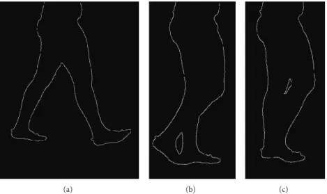
to obtain the silhouette (Figure 1) and the segmental markers

contours.

2.3. Cycle Segmentation and Gait Parameters Determination. Heel strike and toe off events were automatically estimated using a method originally developed for marker-based

sys-tems [29] and adapted to our ML method. Per each time

frame, the centroids of the pelvis and both feet were deter-mined. The gait events (heel strike and toe off) instants were determined when the maximum horizontal relative distance between the pelvis and the foot centroids is achieved.

An expert operator manually identified the same gait events, using the video footage and the heel and toe 3D marker trajectories as reference. The following spatial and temporal parameters were then calculated for both ML and marker-based data: cadence, walking speed, stride time, and stride length. The estimated parameters were compared for validation purposes.

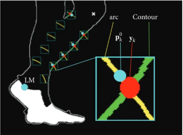
2.4. Model Calibration. A subject-specific, multisegmental model of the lower limb, was used to track the segments and to compute the relevant joint kinematics. The model is made of four segments (foot, tibia, femur, and pelvis) connected by hinges. The position of the following anatomical landmarks was manually identified by the operator in the static reference image: lateral malleolus (LM), lateral femoral epicondyle

(LE), and greater trochanter (GT) (Figure 2(a)).

The foot model template was defined as the posterior half of the foot segmental marker contour. The anatomical

coordinate system (CS_A) of the foot was defined on the

foot model template, with the positive 𝑥-axis coincident

with the line fitting the lower-posterior contour and oriented towards the toes. The origin was made to coincide with the most posterior point of the foot segmental marker contour.

A technical coordinate system (CS_T) was defined with the

𝑥-axis coinciding with the corresponding axis of the CS_I

and centred in LM (Figure 2(b)). The transformation matrix

between the CS_Tand CS_Aof the foot was computedfCSAT

fCST.

The CS_Aof the tibia was defined with the𝑦-axis joining

LM with LE (origin on LM). The tibia model template was defined based on ten reference points identified on the

(3)

(a) (b) (c)

Figure 1: Contour extraction and silhouette contour deformation for three different gait cycle percentages. It can be noticed that in cases (b) and (c) there is an overlap between the foreground and background legs that prevents the identification of the correspondent boundaries of the segments. PL GT LE LM rsh,k rti,k (a) LM CST CSA (b) PLfirst PPfirst PLlast PPlast (c)

Figure 2: (a) Anatomical landmarks and anatomical coordinate systems (CS_A) for the segments analyzed; femur CS_A(yellow axes) and femur reference points (yellow points) identified by the yellow arcs; tibia CS_A(cyan axes) and tibia reference points (cyan points) identified by the cyan arcs. (b) Foot CS_Aand model template. (c) Double anatomical calibration of the most lateral point (PL) in the first and last frame of the gait cycle.

silhouette as the intersections between the shank contour and

the circles of radius𝑟sh,𝑘, centered in LM (Figure 2(a)). The

length of the imposed radii was chosen so that the reference points would fall within the middle portion of the shank segment (between the 25% and 75% of the segment length). This avoided the reference points to fall on the portions of the segment adjacent to the joints. These areas are, in fact,

subject to a larger soft tissue deformation during gait [2]. The

tibia CS_Twas defined with the𝑥-axis parallel to the 𝑥-axis

of the CS_Iand centred in the centroid of the tibia reference

points. The transformation matrix between CS_Tand CS_Aof

the tibia was computedtibCSAT

tibCST(Figure 2(a)). LM and LE

positions and the tibia reference points were then expressed

in the tibia CS_T(tibCSTp0

𝑘,𝑘 = 1, . . . , 10).

The CS_Aof the femur was defined with the𝑦-axis joining

LE with GT (origin on LE). The femur model template was defined based on six reference points identified on the silhouette as the intersections between the thigh contour and

the circles of radius𝑟th,𝑘, centered in LE (Figure 2(a)). The

femur CS_Twas defined with the𝑥-axis parallel to the 𝑥-axis

of the CS_Iand centred in the centroid of the thigh reference

points. The transformation matrix between the CS_Tand CS_A

of the femur was computedfemCSAT

femCST (Figure 2(a)). LE

and GT positions and the femur reference points were then

expressed in the femur CS_T(femCSTp0

𝑘,𝑘 = 1, . . . , 6).

The pelvis CS_A origin was set in the most lateral

point (PL) of the pelvis segmental marker upper contour

(4)

the portion of the pelvis segmental marker upper contour

defined from PL ± 20 pixels and pointing towards the

direction of progression. Due to both parallax effect and pelvis axial rotation during gait, the shape of the pelvis segmental marker changes remarkably throughout the gait

cycle (Figure 2(c)). To improve the quality of the PL tracking

process, a double calibration approach was implemented. At the first and last frames of the gait cycle, the PL positions were

manually identified by the operator (PL_first, PL_last) whereas

the positions of the most posterior point (PP_firstand PP_last)

of the pelvis upper contour were automatically identified.

The horizontal distances between PL_first and PP_first (𝑑_𝑥,first)

and between PL_last and PP_last (𝑑_𝑥,last) were calculated and

the incremental frame by frame variationΔ was computed

according to

Δ =󵄨󵄨󵄨󵄨𝑑𝑥,last− 𝑑𝑥,first󵄨󵄨󵄨󵄨

𝑀 , (1)

with𝑀 representing the number of frames.

The incremental frame variation was then used to

com-pute the distance 𝑑_𝑥,𝑖 between the points PP and PL in

correspondence of the𝑖th frame:

𝑑_𝑥,𝑖= 𝑑_𝑥,first+ (Δ ⋅ 𝑖) . (2)

The position of PL at the𝑖th instant (PL_𝑖) was determined

from the automatically detected position of PP at the same

time instant (PP_𝑖):

PL_𝑖= PP_𝑖+ 𝑑_𝑥,𝑖. (3)

2.5. Dynamic Processing. The dynamic trials were processed using a bottom-up tracking approach, starting from the foot and moving up the chain. The foot was tracked using an iterative contour subtraction matching technique between

the contour at the𝑖th frame and the template foot contour.

At the 𝑖th frame, the foot CS_T was rotated and translated

around the prediction of the LM position based on its velocity estimated in the previous two frames. To make the process more efficient, the rotational span limits were defined based

on the gait cycle phase:±10 degrees during the stance phase

and±30 degrees during the swing phase. The transformation

matrix fCSTT(𝑖)

fCSI between the foot CST and the CSI was

determined by maximizing the superimposition between the

foot template and the foot contour at the𝑖th frame (i.e., the

minimum number of active pixels resulting from the image subtraction). The transformation matrix between the foot

CS_Aand the CS_Iwas computed as

fCSAT (𝑖) fCSI= fCSAT (𝑖) fCST⋅ fCSTT (𝑖) fCSI. (4)

Due to leg superimposition and soft tissues deformation, the silhouette contours of the shank and thigh change during

the gait cycle, making the tracking difficult (Figure 1). To

overcome this issue, the following procedure was adopted for

the tibia. At the𝑖th frame, a registration of first approximation

between the tibia CS_Tand the CS_Iwas carried out using the

position of LM and the prediction of LE. An approximated estimate of the tibia reference points positions with respect

Contour arc LM 𝐲k 𝐩0 k

Figure 3: Tibia reference points detection. These points are identi-fied on the silhouette as the intersections between the shank contour and the circles of radius𝑟_sh,𝑘, centered in LM. LM (cyan circle); predicted LE (white cross); magnified: arc of circumference of radius 𝑟sh,𝑘(yellow curve);y𝑘: reference point detected in the current frame

(red circle);p0_𝑘: template reference point after fitting (cyan circle); silhouette contour line (contour).

to the CS_Iwas then obtained and a 10× 10 pixels region of

interest was created around each point. The final reference

position vectors CSIy

𝑘 of the tibia were detected as the

intersection, where available, between the portion of the shank contour included in the region of interest, and the

circle of radius𝑟tib,𝑘. The transformation matrixtibCSTT(𝑖)tibCSI

between the CS_Iand CS_T was determined using a Singular

Value Decomposition procedure [25] between the position

vectorstibCSTp0

𝑘and the corresponding pointstibCSIy0. Due to

leg superimposition, the number of pointstibCSTp0

𝑘involved

in the fitting procedure varied according to the number of

intersectionstibCSIy

0available (Figure 3). The transformation

matrix between the tibia CS_Aand the CS_Iwas computed as

tibCSAT (𝑖) tibCSI = tibCSAT (𝑖) tibCST⋅ tibCSTT (𝑖) tibCSI. (5)

An identical procedure was employed to determine the

transformation between the CS_I and CS_A of the femur

femCSAT(𝑖)

femCSIat the𝑖th frame.

From the relevant transformation matrices, the joint angles between the pelvis and the femur (hip flex/ext.), between the femur and the tibia (knee joint flex/ext.), and between the tibia and the foot (ankle joint flex/ext.) were computed.

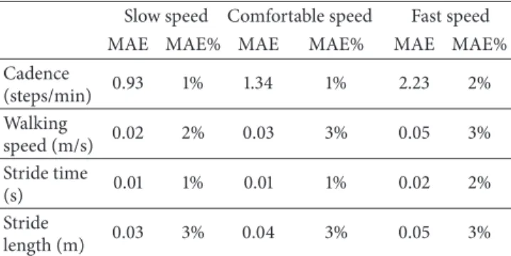
2.6. Data Analysis. For each gait speed, the accuracy of the spatiotemporal gait parameters estimated by the ML approach was assessed in terms of the mean absolute error

(MAE) and MAE% over trials and subjects (3× 10 trials).

Both the ML and marker-based angular kinematic curves were filtered using a fourth-order Butterworth filter (cut-off frequency at 10 Hz). The sagittal angular kinematics produced

by the Plug in Gait protocol was used as gold standard [26].

The kinematic variables were time-normalized to the gait cycle. Furthermore, for each gait trial and each joint,

(5)

Table 1: Gait spatiotemporal parameters. Mean absolute (MAE) and percentage errors of the cadence, walking speed, stride time, and stride length for different gait speeds (slow, comfortable, and fast).

Slow speed Comfortable speed Fast speed

MAE MAE% MAE MAE% MAE MAE%

Cadence (steps/min) 0.93 1% 1.34 1% 2.23 2% Walking speed (m/s) 0.02 2% 0.03 3% 0.05 3% Stride time (s) 0.01 1% 0.01 1% 0.02 2% Stride length (m) 0.03 3% 0.04 3% 0.05 3%

the average root-mean-square deviation (RMSD) value between the joint kinematic curves estimated by the ML method and the gold standard were computed over the gait cycle and averaged across trials and subjects. The similarity between the curves provided by the ML method and the gold standard was assessed using the linear-fit method proposed

by Iosa and colleagues [30]. The kinematic curves produced

by the ML system were plotted versus those produced by the gold standard, and the coefficients of the linear interpolation were used to compare the curves in terms of shape similarity

(𝑅2), amplitude (angular coefficient,𝐴0), and offset (constant

term,𝐴1). The average of 𝐴0 and 𝐴1 across trials and subjects

was calculated for each gait speed.

3. Results

The results relative to the spatiotemporal gait parameters are

shown in Table 1. For all parameters and gait speeds, the

errors were between 1% and 3% of the corresponding true values.

Results relative to the joint kinematics are shown in

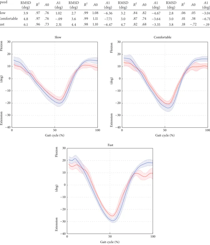
Table 2. Average RMSD values, over trials and subjects,

ranged from 3.9 deg to 6.1 deg for the hip, from 2.7 deg to 4.4 deg for the knee, from 3.0 deg to 4.7 deg for the ankle, and from 2.8 deg to 3.8 deg for the pelvic tilt.

The results of the linear-fit method (𝑅2_{) highlighted}

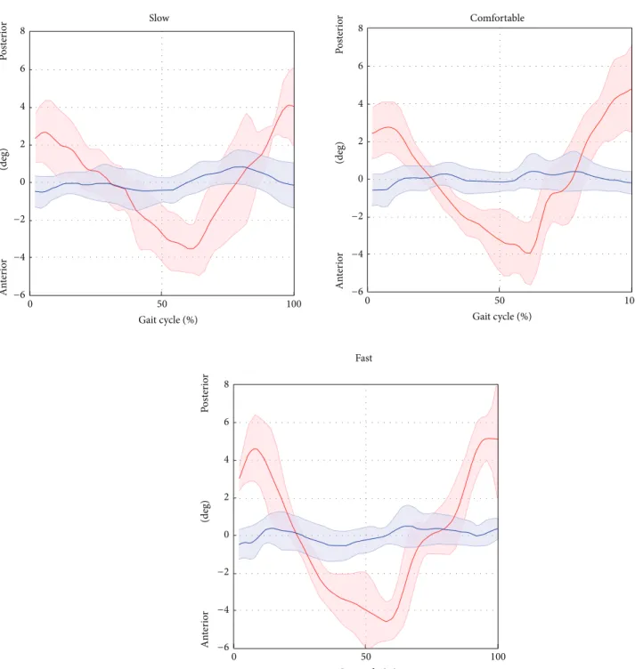
excellent correlation (from 0.96 to 0.99 for all gait speeds) for hip and knee joint kinematics. The ankle kinematics showed strong correlation (from 0.82 to 0.87 for all gait speed). Conversely, the pelvic tilt showed no correlation. The hip and ankle joint kinematics were underestimated in terms of amplitude (𝐴0 ranged from 0.73 to 0.76 and from 0.82 to 0.87 for the hip and ankle, resp.), whereas the knee kinematics were overestimated (𝐴0 from 1.08 to 1.11). The values of the

offset𝐴1 were consistent amongst the different gait speeds

(maximum difference of 2.4 deg for the hip joint, across all

gait velocities) and ranged from −0.1 deg to 2.3 deg, from

−7.7 deg to −6.4 deg, and from −4.7 deg to −3.3 deg for the hip, knee, and ankle, respectively. The joint kinematics and pelvic tilt curves, averaged over trials and subjects and normalised

to the gait cycle, are reported in Figures4,5,6, and7.

4. Discussion and Conclusion

The aim of this study is to implement and validate a ML method based on the use of a single RGB camera for lower limb clinical gait analysis (SEGMARK method). The estimated quantities consist of hip, knee, and ankle joint kinematics in the sagittal plane, pelvic tilt, and spatiotemporal parameters of the foreground limb. The SEGMARK method is based on the extraction of the lower limbs silhouette and the use of garment segmental markers for the tracking of the foot and pelvis.

Key factors of the proposed method are the use of anatomically based coordinate systems for the joint kinemat-ics description, the automatic management of the superim-position between the foreground and background legs, and a double calibration procedure for the pelvis tracking.

For a clinically meaningful description of the joint kine-matics, it is required, for each bone segment, to define a coordinate system based on the repeatable identification of

anatomical landmarks [31]. In our method, the anatomical

calibration is performed by an operator on the static reference image, by clicking on the relevant image pixels. Although it might sound as a limitation, the manual anatomical landmarks calibration is a desired feature because it allows the operator to have full control on the model definition.

When using a single RGB camera for recording gait, the contours of the foreground and background legs are projected onto the image plane, and their superimposition makes difficult the tracking of the femur and tibia segments

during specific gait cycle phases (Figure 1). To overcome

this problem, the model templates of the femur and tibia segments were matched, for each frame, to an adaptable set of target points automatically selected from the thigh and shank contours.

The use of a silhouette-based approach implies that no information related to the pixel greyscale intensity or color values are exploited, except for the background subtraction

procedure [7,8]. This should make the method less sensitive

to change in light conditions or cameras specifications [7,8].

The accuracy with which the spatiotemporal parameters

are estimated (Table 1) is slightly better than other ML

methods [14, 15]. Furthermore, the percentage error was

always lower than 3%. The errors associated to the gait temporal parameter (stride time) estimation were less than 0.02 s, for all gait speeds.

The kinematic quantities estimated by the SEGMARK method and those obtained using a clinically validated gait analysis protocol were compared in terms of

root-mean-square deviation (RMSD), shape (𝑅2_{), amplitude (𝐴0), and}

offset (𝐴1) (Table 2). In this respect, it is worth noting that

the differences found are not entirely due to errors in the joint kinematics estimates, but also to the different definitions used

for the CS_A and the different angular conventions adopted

(2D angles versus 3D Euler angles).

Overall, the RMSD values ranged between 2.7 and 6.1 deg across joints and gait speeds. The smallest RMSD values were found for the knee joint kinematics, followed by the hip and ankle joints kinematics. We reckon that the differences

(6)

Table 2: Lower limb joint and pelvis kinematics. The average root-mean-square deviation (RMSD) value between the joint kinematics curves estimated by the ML method and the gold standard are computed over the gait cycle and averaged across trials and subjects. The similarity between the curves obtained with the proposed ML method and the gold standard is assessed using the linear-fit method [25]. The coefficients of the linear interpolation were used to compare the curves in terms of shape similarity (𝑅2_{), amplitude (angular coefficient,}_{𝐴0), and offset}

(constant term,𝐴1). The average of 𝐴0 and 𝐴1 across trials and subjects is calculated for each gait speed.

Speed

Hip Knee Ankle Pelvis

RMSD (deg) 𝑅 2 _𝐴0 𝐴1 (deg) RMSD (deg) 𝑅 2 _𝐴0 𝐴1 (deg) RMSD (deg) 𝑅 2 _𝐴0 𝐴1 (deg) RMSD (deg) 𝑅 2 _𝐴0 𝐴1 (deg) Slow 3.9 .97 .76 1.02 2.7 .99 1.08 −6.36 3.2 .84 .82 −4.67 2.8 .06 .05 −3.04 Comfortable 4.8 .97 .76 −.09 3.6 .99 1.11 −7.71 3.0 .87 .74 −3.64 3.0 .01 .38 −6.71 Fast 6.1 .96 .73 2.31 4.4 .98 1.10 −6.47 4.7 .82 .68 −3.35 3.8 .18 −.72 −.19 Slow Fast Comfortable 30 20 10 0 0 0 0 Ext en sio n Flexio n 100 50 0 50 100 0 50 100 −10 −20 −30 −40 30 20 10 −10 −20 −30 −40 30 20 10 −10 −20 −30 −40 (deg) Ext en sio n Flexio n (deg) Ext en sio n Flexio n (deg)

Gait cycle (%) Gait cycle (%)

Gait cycle (%)

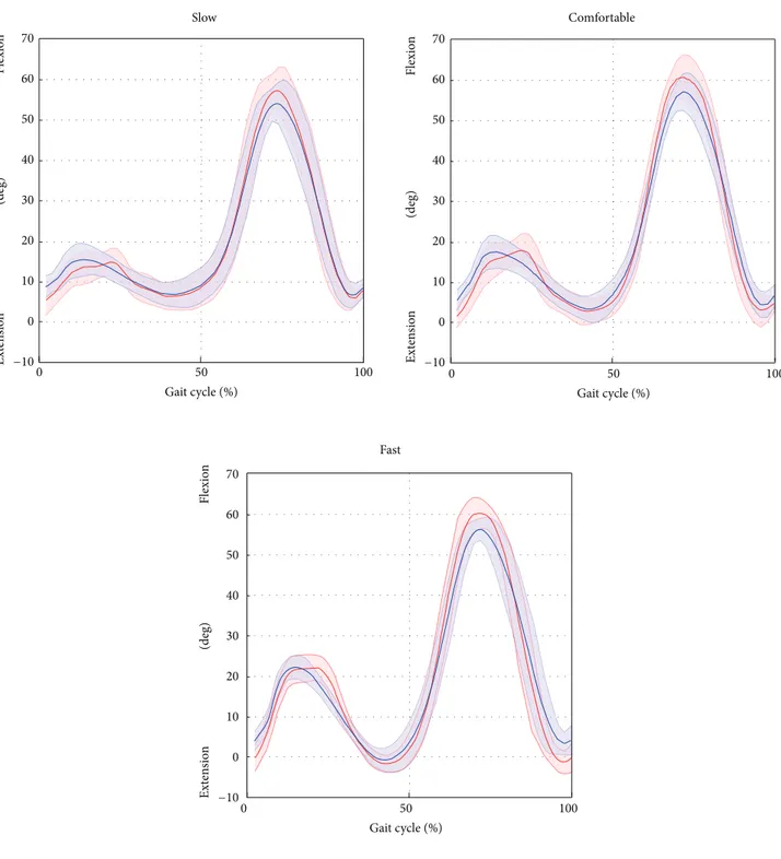
Figure 4: Hip flexion/extension averaged over subjects and trials for the selected gait speed (average: solid lines; SD: shaded area; red = ML; blue = Plug in Gait protocol).

(7)

Slow Fast Comfortable Flexio n 0 50 100 (deg) Gait cycle (%) 0 50 100 Gait cycle (%) 0 50 100 Gait cycle (%) 70 60 40 50 30 20 10 0 −10 70 60 40 50 30 20 10 0 −10 70 60 40 50 30 20 10 0 −10 Flexio n (deg) Flexio n (deg) Ext en sio n Ext en sio n Ext en sio n

Figure 5: Knee flexion/extension averaged over subjects and trials for the selected gait speed (average: solid lines; SD: shaded area; red = ML; blue = Plug in Gait protocol).

at the hip angle between the SEGMARK method and the Plug in Gait model were mainly due to inaccuracies in the pelvis tracking, which proved to be a critical aspect of the single-camera technique proposed. This is mainly due to intrinsic difficulties associated to the pelvis tracking, such as the small range of motion in the sagittal plane during gait (<5 deg), the wider range of motion in the frontal and horizontal planes, and the difficulty to isolate the pelvis from the lower trunk. The differences in the ankle joint kinematics

observed between the SEGMARK method and the Plug in

Gait model (Table 2) can be probably ascribed to the 2D

tracking of the foot segment. In fact, the SEGMARK method cannot account for the foot motion in the transverse plane, leading to an underestimation of the ankle joint motion amplitude (𝐴0 varied from 0.82 to 0.68 for increasing gait speed). The waveform similarity analysis highlighted that the amplitude of the knee joint angle was consistently overes-timated (𝐴0 equals to 1.11 for comfortable speed) whereas

(8)

Slow Fast Comfortable 0 50 100 P la n ta r D o rsiflexio n (deg) Gait cycle (%) 0 50 100 Gait cycle (%) 0 50 100 Gait cycle (%) 15 10 −10 −25 −20 −15 0 5 0 5 P la n ta r D o rsiflexio n (deg) P la n ta r D o rsiflexio n (deg) −5 15 10 −10 −25 −20 −15 −5 0 5 15 10 −10 −25 −20 −15 −5

Figure 6: Ankle plantar/dorsiflexion averaged over subjects and trials for the selected gait speed (average: solid lines; SD: shaded area; red = ML; blue = Plug in Gait protocol).

the hip and ankle joint kinematic curves were consistently underestimated (𝐴0 equals to 0.76 and 0.74 for hip and ankle, resp., for comfortable speed). This can be explained by the consistent overestimation of the pelvis motion, which was in phase with the femur angular displacement, combined with the underestimation of the foot motion in the sagittal plane. An increase of the gait speed showed a negative effect on the accuracy of the kinematics estimation for all the joints due to the significantly smaller number of frames recorded at the

fast gait (≈40 frames) compared to the slow gait (≈80 frames). This result underlines the importance of a sufficiently high frame rate when recording the video footage.

To our knowledge, amongst the 2D ML methods for clinical gait analysis proposed in the literature, just a few use

anatomically relevant points to define the CS_A [22,32,33].

Goffredo and colleagues [22] used an approach based on

skeletonisation and obtained the proportions of the human

(9)

Slow Fast Comfortable 0 50 100 0 50 100 (deg) Gait cycle (%) Gait cycle (%) 0 50 100 Gait cycle (%) 8 6 4 2 0 −4 −6 An te ri o r P o st er io r (deg) 8 6 4 2 0 −4 −6 An te ri o r P o st er io r (deg) 8 6 4 2 0 −4 −6 An te ri o r P o st er io r −2 −2 −2

Figure 7: Pelvic tilt averaged over subjects and trials for the selected gait speed (average: solid lines; SD: shaded area; red = ML; blue = Plug in Gait protocol).

although completely automatic, neglects the subject-specific characteristics, possibly leading to joint angles estimation inaccuracies. Other recent ML validation studies rely upon the built-in algorithm of the Microsoft Kinect to identify joint

centres [33,35], which are therefore not based on anatomical

information, making the use of such techniques questionable for clinical applications. Another important limitation of the 2D ML methods previously proposed is the lack of a systematic validation via a well-established gold standard for

clinical gait analysis applications [13–19]. To our knowledge,

only the work presented by Majernik [32] compared the

joint kinematics with the sagittal plane joint angles produced by a simultaneously captured 3D marker-based protocol. However, neither reference to the specific clinical gait analysis protocol used nor a quantitative assessment of the method performance is reported. Similarly, Goffredo and colleagues

[22] only performed a qualitative validation of their method

(10)

patterns taken from the literature. Moreover, none of the abovementioned works described the procedure used to track the pelvis, which is critical for the correct estimation of the hip joint angle.

Interestingly, when comparing our results with the joint sagittal kinematics obtained from more complex 3D ML techniques, we found errors either comparable or smaller.

Specifically, Sandau et al. [3] reported a RMSD of 2.6 deg for

the hip, 3.5 deg for the knee, and 2.5 deg for the ankle, which

are comparable with the RMSD values reported inTable 2for

the comfortable gait speed. Ceseracciu et al. [4] reported a

RMSD of 17.6 deg for the hip, 11.8 deg for the knee, and 7.2 deg for the ankle, sensibly higher than the values reported in this work. This further confirms the potential of the SEGMARK approach for the study of the lower limb motion in the sagittal plane for clinical applications.

This study has limitations, some of them inherent to the proposed ML technique, whereas others related to the experimental design of the study. First, the joint kinematics is only available for the limb in the foreground, while other authors managed to obtain a bilateral joint kinematics

description using a single camera [22]. Therefore, to obtain

kinematics from both sides, the subject has to walk in both directions of progression. Second, the segmentation procedure for the subject silhouette extraction takes advan-tage of a homogeneous blue background. This allows for optimal segmentation results, but it adds a constraint in the experimental setup. For those applications where the use of a uniform background is not acceptable, more advanced

segmentation techniques can be employed [7–9]. Finally, the

anatomical calibration procedure requires the operator to visually identify the anatomical landmarks in the static image, and this operation necessarily implies some repeatability errors which would need to be assessed in terms of inter and

intra observer and inter and intrasubject variability [35]. As

a future step, the present methodology will be applied and validated on pathological populations such as cerebral palsy children.

Conflict of Interests

The authors declare that there is no conflict of interests regarding the publication of this paper.

References

[1] R. Baker, “Gait analysis methods in rehabilitation,” Journal of NeuroEngineering and Rehabilitation, vol. 3, article 4, 2006. [2] U. Della Croce, A. Leardini, L. Chiari, and A. Cappozzo,

“Human movement analysis using stereophotogrammetry part 4: assessment of anatomical landmark misplacement and its effects on joint kinematics,” Gait & Posture, vol. 21, no. 2, pp. 226–237, 2005.

[3] M. Sandau, H. Koblauch, T. B. Moeslund, H. Aanæs, T. Alkjær, and E. B. Simonsen, “Markerless motion capture can provide reliable 3D gait kinematics in the sagittal and frontal plane,” Medical Engineering & Physics, vol. 36, no. 9, pp. 1168–1175, 2014.

[4] E. Ceseracciu, Z. Sawacha, and C. Cobelli, “Comparison of markerless and marker-based motion capture technologies through simultaneous data collection during gait: proof of concept,” PLoS ONE, vol. 9, no. 3, Article ID e87640, 2014. [5] S. Corazza, L. M¨undermann, E. Gambaretto, G. Ferrigno, and

T. P. Andriacchi, “Markerless motion capture through visual hull, articulated ICP and subject specific model generation,” International Journal of Computer Vision, vol. 87, no. 1-2, pp. 156–169, 2010.

[6] L. M¨undermann, S. Corazza, A. M. Chaudhari, T. P. Andri-acchi, A. Sundaresan, and R. Chellappa, “Measuring human movement for biomechanical applications using markerless motion capture,” in 7th Three-Dimensional Image Capture and Applications, vol. 6056 of Proceedings of SPIE, p. 60560R, International Society for Optics and Photonics, San Jose, Calif, USA, January 2006.

[7] L. M¨undermann, S. Corazza, and T. P. Andriacchi, “The evolu-tion of methods for the capture of human movement leading to markerless motion capture for biomechanical applications,” Journal of NeuroEngineering and Rehabilitation, vol. 3, article 6, 2006.

[8] T. B. Moeslund and E. Granum, “A survey of computer vision-based human motion capture,” Computer Vision and Image Understanding, vol. 81, no. 3, pp. 231–268, 2001.

[9] H. Zhou and H. Hu, “Human motion tracking for rehabilitation—a survey,” Biomedical Signal Processing and Control, vol. 3, no. 1, pp. 1–18, 2008.

[10] A. Harvey and J. W. Gorter, “Video gait analysis for ambulatory children with cerebral palsy: why, when, where and how!,” Gait & Posture, vol. 33, no. 3, pp. 501–503, 2011.

[11] U. C. Ugbolue, E. Papi, K. T. Kaliarntas et al., “The evaluation of an inexpensive, 2D, video based gait assessment system for clinical use,” Gait & Posture, vol. 38, no. 3, pp. 483–489, 2013. [12] J.-H. Yoo and M. S. Nixon, “Automated markerless analysis of

human gait motion for recognition and classification,” ETRI Journal, vol. 33, no. 2, pp. 259–266, 2011.

[13] R. A. Clark, K. J. Bower, B. F. Mentiplay, K. Paterson, and Y.-H. Pua, “Concurrent validity of the Microsoft Kinect for assess-ment of spatiotemporal gait variables,” Journal of Biomechanics, vol. 46, no. 15, pp. 2722–2725, 2013.

[14] N. Vishnoi, Z. Duric, and N. L. Gerber, “Markerless identifica-tion of key events in gait cycle using image flow,” in Proceedings of the Annual International Conference of the IEEE Engineering in Medicine and Biology Society (EMBC ’12), pp. 4839–4842, 2012.

[15] N. R. Howe, M. E. Leventon, and W. T. Freeman, “Bayesian reconstruction of 3D human motion from single-camera video,” in Advances in Neural Information Processing Systems, pp. 820– 826, MIT Press, 1999.

[16] D. K. Wagg and M. S. Nixon, “Automated markerless extraction of walking people using deformable contour models,” Computer Animation and Virtual Worlds, vol. 15, no. 3-4, pp. 399–406, 2004.

[17] C. Bregler and M. Jitendra, “Tracking people with twists and exponential maps,” in Proceedings of the IEEE International Conference on Computer Vision and Pattern Recognition, 1998, pp. 8–15, Santa Barbara, Calif, USA, June 1998.

[18] M. Enzweiler and D. M. Gavrila, “Monocular pedestrian detec-tion: survey and experiments,” IEEE Transactions on Pattern Analysis and Machine Intelligence, vol. 31, no. 12, pp. 2179–2195, 2009.

(11)

[19] J. E. Boyd and J. J. Little, “Biometric gait recognition,” in Advanced Studies in Biometrics, vol. 3161 of Lecture Notes in Computer Science, pp. 19–42, Springer, Berlin, Germany, 2005. [20] E. Surer, A. Cereatti, E. Grosso, and U. D. Croce, “A markerless

estimation of the ankle-foot complex 2D kinematics during stance,” Gait & Posture, vol. 33, no. 4, pp. 532–537, 2011. [21] A. Schmitz, M. Ye, R. Shapiro, R. Yang, and B. Noehren,

“Accuracy and repeatability of joint angles measured using a single camera markerless motion capture system,” Gait & Posture, vol. 47, pp. 587–591, 2014.

[22] M. Goffredo, J. N. Carter, and M. S. Nixon, “2D markerless gait analysis,” in Proceedings of the 4th European Conference of the International Federation for Medical and Biological Engineering, vol. 22 of IFMBE Proceedings, pp. 67–71, Springer, Berlin, Germany, 2009.

[23] J. Saboune and F. Charpillet, “Markerless human motion cap-ture for gait analysis,”http://arxiv.org/abs/cs/0510063. [24] A. Leu, D. Ristic-Durrant, and A. Graser, “A robust markerless

vision-based human gait analysis system,” in Proceedings of the 6th IEEE International Symposium on Applied Computational Intelligence and Informatics (SACI ’11), pp. 415–420, Timisoara, Romania, May 2011.

[25] F. E. Veldpaus, H. J. Woltring, and L. J. M. G. Dortmans, “A least-squares algorithm for the equiform transformation from spatial marker co-ordinates,” Journal of Biomechanics, vol. 21, no. 1, pp. 45–54, 1988.

[26] R. B. Davis III, S. ˜Ounpuu, D. Tyburski, and J. R. Gage, “A gait analysis data collection and reduction technique,” Human Movement Science, vol. 10, no. 5, pp. 575–587, 1991.

[27] J. Heikkila and O. Silv´en, “Calibration procedure for short focal length off-the-shelf CCD cameras,” in Proceedings of the 13th International Conference on Pattern Recognition (ICPR ’96), vol. 1, pp. 166–170, August 1996.

[28] J. F. Canny, “A computational approach to edge detection,” IEEE Transactions on Pattern Analysis and Machine Intelligence, vol. 8, no. 6, pp. 679–698, 1986.

[29] J. A. Zeni Jr., J. G. Richards, and J. S. Higginson, “Two simple methods for determining gait events during treadmill and overground walking using kinematic data,” Gait & Posture, vol. 27, no. 4, pp. 710–714, 2008.

[30] M. Iosa, A. Cereatti, A. Merlo, I. Campanini, S. Paolucci, and A. Cappozzo, “Assessment of waveform similarity in clinical gait data: the linear fit method,” BioMed Research International, vol. 2014, Article ID 214156, 7 pages, 2014.

[31] A. Cappozzo, U. Della Croce, A. Leardini, and L. Chiari, “Human movement analysis using stereophotogrammetry. Part 1: theoretical background,” Gait & Posture, vol. 21, no. 2, pp. 186– 196, 2005.

[32] J. Majernik, “Marker-free method for reconstruction of human motion trajectories,” Advances in Optoelectronic Materials, vol. 1, no. 1, 2013.

[33] M. Gabel, R. Gilad-Bachrach, E. Renshaw, and A. Schuster, “Full body gait analysis with Kinect,” in Proceedings of the 34th Annual International Conference of the IEEE Engineering in Medicine and Biology Society (EMBS ’12), pp. 1964–1967, San Diego, Calif, USA, September 2012.

[34] R. A. Clark, Y.-H. Pua, A. L. Bryant, and M. A. Hunt, “Validity of the Microsoft Kinect for providing lateral trunk lean feedback during gait retraining,” Gait & Posture, vol. 38, no. 4, pp. 1064– 1066, 2013.

[35] M. H. Schwartz, J. P. Trost, and R. A. Wervey, “Measurement and management of errors in quantitative gait data,” Gait & Posture, vol. 20, no. 2, pp. 196–203, 2004.

(12)