Accuracy driven hybrid localization method

(1)

POLITECNICO DI MILANO

Scuola di Ingegneria dell’Informazione

POLO TERRITORIALE DI COMO

Master of Science in Computer Engineering

Accuracy-driven Hybrid Localization Method

Supervisor: Prof. Fabio Salice

Assistant Supervisor: Eng. Fabio Veronese

Master Graduation Thesis by: Majid Farzaneh

Student Id. Number: 780117

Academic Year 2013-2014

(2)

ABSTRACT

The development of communications network and mobile computing, and the increasing demand for location-based services inside buildings, have made indoor positioning a very popular research topic in recent years. Indoor Human Localization (IHL) systems are based on several different technologies, surely the most diffused are based on Radio-Frequencies.

The localization technology exploited in this thesis is based on 2.4 GHz. In order to obtain the physical position of the target-of-interest, the process of localization is divided in two phases: signal measurement and position estimation. In this study in first phase we use received signal strength (RSS) parameter, and in the second phase we used a grid-based lateration method. In order to obtain the distance estimation in the first phase of localization, two different signal propagation models (LAURA and MWM) are exploited, the two methods are evaluated and their performances are presented. Furthermore, based on the complementary performances of the two implemented models, we developed several methods to compose the two algorithms, to provide an improvement of position estimation. The developed methods are divided in two parts: basic methods using a static mixture policy, or using dynamic mixture policy based on estimation accuracy indicators.

The proposed method, based on a policy involving two confidence indicators, provides a combination of LAURA and MWM methods. The policy enables to choose the model at each time instant, which is probable to give better estimations. Experimental data prove the validity of the approach, reporting an improvement in the localization results.

(3)

SOMMARIO

Lo sviluppo di reti di comunicazione e mobile computing, e la crescente domanda per servizi basati su localizzazione in ambienti coperti, hanno reso la localizzazione indoor un importante argomento di ricerca negli ultimi anni. Sistemi di localizzazione di persone indoor (Indoor Human Localization - IHL) sono basati sulle tecnologie più disparate, sebbene i più diffusi si affidino alle Radio Frequenze.

La tecnologia di localizzazione utilizzata in questa tesi è basata su segnali a 2.4GHz. Per ottenere la posizione della persona-target, il processo di localizzazione può essere diviso in due fasi: la raccolta di segnali e la stima della posizione. In questo studio per la prima fase sono stati utilizzati i dati di potenza del segnale ricevuta (Received Signal Strength - RSS), mentre nella seconda un metodo di laterazione basato su una griglia. Per ottenere la stima della distanza nella prima parte del processo di localizzazione, sono stati utilizzati due diversi modelli (LAURA e MWM) di propagazione del segnale; questi modelli sono stati valutati e le loro prestazioni confrontate. Inoltre, partendo dalla complementarietà delle prestazioni di questi due modelli, sono stati sviluppati diversi metodi per combinarne i procedimenti, al fine di raggiungere un miglioramento della posizione stimata. I metodi sviluppati sono stati classificati in due tipologie: basati su strategie di composizione statiche, o dinamiche, basate su indicatori di accuratezza.

(4)

Il metodo proposto, basato su una strategia che coinvolge due indicatori di confidenza, fornisce una combinazione dei metodi Laura e MWM. Questa permette ad ogni istante di tempo, di scegliere il modello che ci si aspetta dia una stima migliore. I dati sperimentali confermano la validità dell'approccio, e riportano un miglioramento nei risultati di localizzazione.

(5)

Table of

List of Figures

Figure 1: Two phases in localization ... 5

Figure 2: Triangulation-based positioning ... 10

Figure 3: Trilateration-based positioning ... 12

Figure 4: Classification of indoor localization technologies by measured physical quantity and hardware technology ... 14

Figure 5: Distribution of articles by physical quantity measured ... 14

Figure 6: One-Slope Model coverage prediction ... 21

Figure 7: Multi-Wall Model coverage prediction ... 23

Figure 8: Fitted Curve based on outdoor experiment ... 28

Figure 9: Histograms for LOS-NLOS comparison ... 29

Figure 10: Map of the building ... 31

Figure 11: ecdf graphs of estimated distance error before lateration ... 34

Figure 12: ecdf graphs of localization error after lateration ... 35

Figure 13: Graphical definition of variables ... 38

Figure 14: ecdf of localization error for the first basic mixture method ... 40

Figure 15: ecdf of localization error for the second basic mixture method ... 41

Figure 16: ecdf of localization error for the third basic mixture method ... 43

Figure 17: The error value and each indicator value for LAURA method in Dataset A ... 47

Figure 18: The error value and each indicator value for MWM method in Dataset A ... 48

Figure 19: The error value and each indicator value for LAURA method in Dataset B ... 50

Figure 20: The error value and each indicator value for MWM method in Dataset B ... 52

Figure 21: ecdf of localization error for the mixture method based on SumVar ... 58

Figure 22: ecdf of localization error for the mixture method based on MED ... 59

Figure 23: ecdf of localization error for the mixture method based on both indicators ... 61

(8)

List of Tables

Table 1: Distances between Wall and devices for NLOS tests ... 29

Table 2: Self Power and Self Distance values ... 30

Table 3: System Parameters ... 31

Table 4: Errors of LAURA and MWM methods for Dataset A ... 33

Table 5: Errors of LAURA and MWM methods for Dataset B ... 33

Table 6: Localization Error of the first basic mixture method ... 39

Table 7: Localization Error of the second basic mixture method ... 40

Table 8: Localization Error of the third basic mixture method ... 42

Table 9: Correlation value between error and indicators in dataset A in LAURA method 47 Table 10: Correlation value between error and indicators in dataset A in MWM method . 49 Table 11: Correlation value between error and indicators in dataset B in LAURA method ... 50

Table 12: Correlation value between error and indicators in dataset B in MWM method . 52 Table13: ROC space analysis results of hypothesis ... 54

Table 14: ROC space analysis results of novel hypothesis ... 56

Table 15: Localization Error of the mixture method based on SumVar indicator ... 57

Table 16: Localization Error of the mixture method based on MED indicator ... 58

Table 17: Localization Error of the mixture method based on both indicators ... 60

Table 18: Localization Error of the second mixture method based on both indicators ... 61

(9)

Glossary

AOA Angle of Arrival

ECDF Empirical Cumulative Distribution Function FN False Negative

FP False Positive

FPR False Positive Rate

GPS Global Positioning System

IHL Indoor Human Localization

LOS Line of Sight

MED Minimum Estimated Distance

MLE Maximum Likelihood Estimation

MWM Multi-Wall Model

NLOS Non Line of Sight RF Radio Frequency

RFID Radio Frequency Identification

RMS Root Mean Square

RTT Round Trip Time

RSS Received Signal Strength

RSSI Received Signal Strength Indication TDOA Time Difference of Arrival

TN True Negative

(10)

TP True Positive

TPR True Positive Rate

UDP Undetected Direct Path

UWB Ultra Wide Band

WLAN Wireless Local Area Network

WSN Wireless Sensor Network

(11)

Chapter 1 Introduction

Introduction

The development of communications network and mobile computing, and the increasing demand for location-based services inside buildings, have made indoor positioning a very popular research topic in recent years. Location-based services refer to applications that rely on the user’s location to provide services, such as advertising, street navigation, public transportation, etc. There are many applications of indoor positioning, for instance, navigation for people or robots, locating patients in a hospital, guiding blind people, tracking elderly people or small children, location based services and etc.

The Global Positioning System (GPS) is the most popular outdoor positioning system, although it cannot provide good accuracy in indoor environments, since its signals are easily blocked by most construction materials. This rises the need for alternative technologies. An example of a possible alternative, is the system exploited in this study, which is based on a 2.4GHz Wireless Sensor Network (WSN). The localization technology relies on Received Signal Strength Indication

(12)

(RSSI) between a mobile node worn by a person and some location-known fixed devices installed inside the building. The signals transmitted travel in the environment, and their attenuation can be exploited to estimate distances. This estimation process can rely on different signal propagation models. In this thesis two different models and their related algorithms are compared, providing experimental evaluation of their performances. Due to the limited accuracy of the analyzed technology, the aim of this work was the development of a novel model, here by presented, enabling the composition of distances estimation obtained through different algorithms, to obtain a better position estimation.

Structure of the Thesis

This thesis is divided into five main chapters. After this introductive chapter, in Chapter 2, we review the state of the art. First we briefly introduce problem formulation, and the localization methods are introduced. Moreover, we describe a classification of indoor localization technologies by measured physical quantity and hardware technology. A classification of Radio Frequency technologies in indoor localization is reported and, the last part, RF signal propagation models are discussed.

In Chapter 3, a detailed description of the localization methods evaluation is provided, along with experiments results about their performances.

In Chapter 4, different mixture methods are introduced in order to improve the localization methods. The results are presented and a full analysis with comparison is included in this chapter.

(13)

Chapter 5 summarizes the conclusion drawn from this thesis, proposing some topics for future work.

(14)

Chapter 2 Indoor Human Localization (IHL):

Radio-Frequency Based Technologies

and Methods

Problem Formulation

An Indoor localization system is a system that can determine the position of something or someone, continuously and in real time [4]. In order to obtain the physical position of the target-of-interest, two steps are usually needed [5, 6]: first, some position-related quantities are measured; and then, the physical position of the target is calculated based on the obtained information.

As shown in Figure 1, we can thus divide the whole localization process into two phases: signal measurement and position calculation. In the first phase, some properties of these signals, such as arrival time (Time of Arrival –ToA– , Time difference of Arrival –TDoA–), signal strength (Received Signal Strength –RSS–), and direction (Angle of Arrival –AOA–), are collected by the receivers.

(15)

Figure 1: Two phases in localization [3].

In the second phase, the physical position of the target is determined based on the parameters obtained. The most common technique used is based on ranging, whereby distance or angle approximations are obtained. In this context, geometric approaches are employed, as further described to calculate the position of the target node from the position-related parameters at reference nodes. Trilateration and triangulation are two most popular geometric approaches. In addition, since signal measurements in real systems are only accurate to some extent (especially in indoor environments), optimization-based statistical techniques are often used to filter measurement noise and improve accuracy of the result.

Distance Estimation Methods

In this section we will explain the most common methods for distance/direction estimation which are involved in the first phase of localization.

The three main categories of methods can be identified: time-based methods; the angle-based methods (AoA); and the third is the received signal strength based methods (RSS).

(16)

A. Time-based Methods 1. Time of Arrival (ToA)

With ToA, the distance between the a node, transmitting a signal, and the receiving node is deduced from the transmission time delay and the corresponding speed of signal as follows:

! = !"#$ × !"##$ (1) where speed denotes the traveling speed of the signal, time the amount of time spent by the signal travelling from the transmitting to the receiving node, and R the distance between the transmitting node and the receiving node. Since speed can be regarded as a known constant, R can be computed by observing time. This implies the necessity to synchronize devices, which often rises technological issues.

The ToA localization suffers from two sources of errors: multipath effects and Undetected Direct Path (UDP) conditions. Multipath effect is caused by obstacles and it results in reflected and transmitted paths, received along with the direct one, hence causing ranging errors. These errors can be reduced by increasing the transmission bandwidth of the system; as the bandwidth increases, the pulses get narrower and the ToA estimate gets closer to the expected ToA of the direct path. The UDP condition occurs when the direct path falls below the detection threshold of the receiver. This condition usually happens at the edges of the coverage area or when the direct path between the transmitter and the receiver is blocked. The UDP condition results in very large ranging errors and cannot be minimized by increasing the bandwidth of the

(17)

transmission system [3].

2. Time Difference-of-Arrival (TDOA)

This technology uses two different transmitted signals. The time difference between these two is used to reconstruct the transmitting node's position. The calculation is based on the following equation:

! !_!−

!

!_! = !!− !! (2) where, c1 denotes the speed of the first signal, c2 the speed of the second, t1 and t2 the time for these two signals travelling from one node to the

other respectively, and R the distance between the transmitting node and the receiving node.

3. Round Trip Time (RTT)

This measurement method emerges with the goal of solving the problem of synchronization incurred by ToA. Instead of using two synchronized nodes to calculate the delay (as ToA technology does), it requires timing on one node only, to record the transmitting and arrival time. With RTT, the distance is calculated as follows:

! = !!"− ∆! × !"##$

2 (3) where !_!" denotes the amount of time needed for a signal to travel from one node to the other and back again, Δt the predetermined time delay required by the hardware device to echo the signal back to the receiving node, and speed the speed of the transmitting signal.

(18)

B. Angle-of-Arrival (AoA)

With respect to AoA-based techniques, the reference nodes or the target node have the capability of measuring the angle of arrival of the signal. For this purpose, techniques like angle diversity [9] may be utilized in order to exploit the directionality of the receiver. Usually, direction finding can be accomplished by either with directional antennas or with an array of antennas. The main principle behind the AoA measurement via antenna arrays consists in the angle information included in differences of arrival times of the incoming signal at different antenna elements. With AoA, no time synchronization between nodes is required.

AoA-based techniques have anyway their limitations. Since AoA-based methods are highly sensitive to multi-path and NLOS (Non-Line-Of-Sight), they are not always suitable for indoor localization. As the distance increases, the localization precision will decrease. In addition, technologies based on AoA require antennas with the capacity to measure the angles, which increases the cost of the whole system.

C. Received Signal Strength (RSS)

For the RSS based techniques, the distance is measured based on the attenuation due to the propagation of the signal from the transmitting node to the receiving node. A mathematical model to calculate the distance according to signal propagation is as follows:

! ! = ! !_! − 10! log !

(19)

where R denotes the distance between the transmitter and the receiver, R0 a

reference distance, p(R) and p(R0) the signal strength received at R and R0

respectively, nW the number of obstacles between the transmitter and the receiver, WAF the attenuation factor of the wall, C the maximum number of obstacles between the transmitter and the receiver, and n the routing attenuation factor which could be determined by both theoretical and empirical calculations.

Based on the RSS technology, several methods have been proposed to estimate the position of the target-of-interest. For example, the fingerprint-based solution for target positioning is one of the most typical application of RSS technology. In general, we can divide the fingerprint methodology into two steps: sampling (offline) and matching (online). In the sampling step, a database is created offline to store the radio signal map consisting of the geographical positions and the corresponding signal strengths. These signals may be e.g. sound, light, color, and human movement, among others. In the matching step, the relevant signals collected for the target (node) are compared against the pre-stored records of the geographic-signal map. By doing so, it will be able to determine where the target is, as long as any record in the database is matched.

(20)

Localization Methods

Based on the quantities estimated in the first phase and the known coordinates of reference nodes, in the second phase of localization it is possible to calculate the physical position of the target. To do this, trilateration and triangulation techniques are commonly used. In addition, statistical techniques could be employed to improve the solution accuracy by coping with measurement noise. In this regard, we will introduce a very popular parametric approach: maximum likelihood estimation, though there are many other approaches in the literature.

A. Triangulation

When AoA measurements are available, triangulation can be used to determine the position of the target node. Triangulation-based positioning is based on the measurement of angles. In most situations, triangulation can be transformed to trilateration since the distance between nodes can be reconstructed from the bearings between them. However, compared to trilateration, only two reference nodes are needed for triangulation (in 2D), instead of three [3].

Figure 2: Triangulation-based positioning

(21)

the intersection of several pairs of angle direction lines. As shown in Figure 2 where A and B represent reference nodes, after obtaining the angles θ1 , and

θ2 , the physical position of T (representing the target to be located) can be

calculated based on the predetermined coordinates of the reference nodes. B. Maximum Likelihood Estimation (MLE)

MLE is a method of estimating the parameters of a statistical model. When applied to a data set and given a statistical model, maximum-likelihood estimation provides estimates for the model's parameters.

The method of maximum likelihood corresponds to many well-known estimation methods in statistics. For example, one may be interested in the heights of adult female penguins, but be unable to measure the height of every single penguin in a population due to cost or time constraints. Assuming that the heights are normally (Gaussian) distributed with some unknown mean and variance, the mean and variance can be estimated with MLE while only knowing the heights of some sample of the overall population. MLE would accomplish this by taking the mean and variance as parameters and finding particular parametric values that make the observed results the most probable (given the model).

In general, for a fixed set of data and underlying statistical model, the method of maximum likelihood selects the set of values of the model parameters that maximizes the likelihood function. Intuitively, this maximizes the "agreement" of the selected model with the observed data, and for discrete random variables it indeed maximizes the probability of the observed data under the resulting distribution. Maximum-likelihood

(22)

estimation gives a unified approach to estimation, which is well-defined in the case of the normal distribution and many other problems.

C. Trilateration

As illustrated in Figure 3, the trilateration based positioning algorithm uses three fixed non-collinear reference nodes to calculate the physical position of a target node (in 2D) [3].

Figure 3: Trilateration-based positioning

Based on the coordinates of three reference nodes: A(x1, y1), B(x2, y2), and

C(x3, y3), and the corresponding distances from each reference node to the

target node: R1 , R2 , and R3 , we can obtain the following equations:

!_!− ! !_{+ !} !− ! ! = !!! !_!− ! !_{+ !} !− ! ! = !!! !_!− ! !_{+ !} !− ! ! = !!! (5)

where (x, y) denotes the (unknown) coordinates of the target T.

We can see that the trilateration algorithm can best demonstrate its advantages when the three reference nodes are deployed in the vertices of equilateral triangles. Also some other studies consider the effect of noisy environments, and use different confidence coefficients for three nodes to

(23)

guarantee the quality of trilateration. In case more than three measurements can be exploited, a variant of trilateration is raised which is multilateration. D. Lateration (Grid Based)

This method relies on a grid of points, defined selecting the dimension of its atomic unit [1]. We leverage the known distance between each point of the grid and each anchor node, selecting the target location as the grid point that minimizes the discrepancy. The best point of the grid is computed as:

! = argmin

!"# !!− !! !− !! ! !"#

(6)

where ! is the set of grid nodes, ! the set of fixed devices, !! the estimated

distance from the l-th anchor, !_! and !_! the coordinates of the i-th node of the grid and the l-th anchor.

Physical Quantity Classification

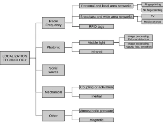
Modern indoor localization systems use many different and various techniques. The location of an object in space is determined by measuring a physical quantity that changes proportionally with the position of the object of interest. We can report a classification for localization technologies on the basis of that measured quantity. In particular, we can identify the following classes: Radio frequency waves, photonics energy, sonic waves, mechanical energy (inertial or contact), magnetic fields, and atmospheric pressure. Each one can be further subdivided according to the underlying hardware technology. Figure 4 summarizes this classification [12]:

(24)

Figure 4: Classification of indoor localization technologies by measured physical quantity and hardware technology

Moreover it is possible to highlight the distribution of research over these technologies by considering the number of articles for each physical quantity measured [12] in Figure 5:

(25)

This work mostly focuses on Radio Frequency waves field and its subcategories. Next sections will explain each of these sub-categories briefly, focusing then on the known localization methods.

Technology and Frequency Classification

An electromagnetic wave is the energy generated by an oscillating, electrically charged particle in space. The generation of electromagnetic waves is known as a radio frequency emission.

Radio Frequency travels in the space at a known speed, and their power decays as they get further from their space. The location of a mobile target in this category is estimated and calculated by measuring one or more properties of a wave radiated by a transmitter and received by a mobile station.

We can divide radio frequency category in different subcategories according to the underlying technology and frequency:

1. IEEE 802.11(WLAN), 802.15.4(ZigBee): The localization technique used for positioning with wireless access points is based on measuring the received signal strength (RSS). Furthermore, 2.4 GHz technologies can be used with other distance estimation metrics such as time-based methods (ToA, TDoA) and Angle-of-Arrival (AoA) method. Typical parameters useful to geolocate the WiFi hotspot or wireless access point include the SSID and the MAC address of the access point. The accuracy depends on the number of positions that have been entered into the database. The

(26)

possible signal fluctuations that may occur can increase errors and inaccuracies in the path of the user. WLAN is used where GPS is inadequate. 2. Bluetooth: Bluetooth in often employed for indoor proximity rather than indoor positioning. A Bluetooth device inquires about neighboring Bluetooth stations [13]. This inquiry process consists of scanning for devices in the vicinity, using a sequence of different power levels. Low power levels will detect devices in close proximity while high power levels will include devices that are located farther away, providing coarse distance estimates in this fashion. This approach requires a fixed or anchor node which establishes the position of nearby mobile nodes. Subsequently, the localized nodes can establish the position of other undetected mobiles nodes in their vicinity, creating an ad-hoc localization network

3. Ultra Wide Band (UWB): UWB has very high precision, approximately 15 cm for 95% of the readings thanks to the active tags signal triangulation [14]. Usually the main components of an UWB system are: the sensors, the tags to be tracked and the software platform. The tags use RF Radio to coordinate the UWB (6–8 GHz) pulse transmission time. An UWB system uses different signal measurement methods in order to estimate the location of a specific tag using at least two receivers. These systems do not require Line-of-Sight thanks to the UWB technology. The signal can be filtered and the multipath effect minimized, which is huge advantage because the multipath effect represents the main cause for low accuracy indoors. UWB systems can cover large areas and offers the possibility of tracking a large number of user in real-time. The spatial coverage is ensured using cluster methods running a

(27)

large number of services with a fair usage of bandwidth. A drawback of UWB systems is the timing cable required for every tag which can become challenging in some environments.

4. Radio Frequency Identification (RFID) tags: An RFID system is commonly composed of one or more reading devices that can wirelessly obtain the ID of tags present in the environment [15]. The reader transmits a RF signal. The standard RFID frequency bands are listed as: 120-150 kHz (LF), 13.56 MHz (HF), 433 MHz (UHF), 865-866 MHz in Europe (UHF), 902-928 MHz in North America (UHF). The tags present in the environment reflect the signal, modulating it by adding a unique identification code. The tags can be active (powered by a battery), or passive, drawing energy from the incoming radio signal. The detection range of passive tags is therefore more limited.

5. Radar: An example of Radar-based localization is presented by Roehr [16]. He presented an extension to the conventional frequency-modulated continuous-wave radar. The particular characteristic of this system is that it uses two-way radio communication. Both fixed and mobile units are capable of transmitting and receiving a frequency modulated signal with a 5.8 GHz carrier. The fixed and mobile clocks are synchronized before distance and velocity estimations could be calculated. Once the units are synchronized, the fixed unit emits a signal, which arrives at the mobile station. Subsequently, the mobile station send a reply to the fixed station, which is synchronized using the signal just receives from the fixed station. The round trip time of the signal is used to calculate the distance between the fixed and

(28)

the mobile stations, while the frequency deviation is used to estimate the velocity of the mobile unit. The experimental setup include one experiment within an office building, where distances ranging from 5 to 25 metres are measured with the radar system.

Signal Propagation Models

The ability to accurately predict radio-propagation behavior for wireless personal communication systems, such as cellular mobile radio, is becoming crucial to system design. Indeed, the prediction of RF signal propagation is necessary to estimate the network coverage. Furthermore, this kind of analysis can provide the information necessary for RSS-based localization methods. Since site measurements are costly, propagation models have been developed as a suitable, low-cost, and convenient alternative, used in the network planning and deployment process.

Over the years, a number of models have been developed for the prediction of radio wave propagation. They can be categorized into two main approaches: empirical and deterministic.

Empirical models are based on vast amounts of actual measurements and they are primarily based on statistically processed representing measurements. Empirical models are very easy and fast to apply because the prediction is usually obtained from simple closed expressions. Also requirements on the input environment description are not so restrictive. At the same time, the propagation loss, with a limited site-specific accuracy, can be predicted. Total path loss LTOT (dB) can be

(29)

!_!"! = ! ! + ! (7) where L(P) (dB) is the average loss based on the position P only, and χ (dB) is random fading with a zero-mean statistical distribution. The empirical models are able to predict the average path loss L(P).

On the other side, deterministic models utilize the laws of electromagnetic waves to determine a number of parameters, including the phase and signal strength of the wave at a particular domain of interest or area. Deterministic models (e.g. Ray Tracing) often require extensive knowledge about the terrain in the form of three dimensional maps, aerial photography or satellite pictures.

In the following, first we explain Ray Tracing as an example of deterministic models and then two wide-spread empirical models: One-Slope and Multi-Wall.

Ray Tracing

Ray tracing model is based on Geometrical Optics (GO). Rays are radio signals. Rays are followed until they hit an object, where a reflected/transmitted ray is initiated in the next reflection/transmission depth [27, 28]. The direction of the new ray is determined by Snellius' law. Losses due to reflections and transmissions take into account the thickness of the hit walls/floors and the material characteristics at the respective frequency. Furthermore, diffracted rays can be considered by means of the Uniform

Theory of Diffraction (UTD). In the frequency range of 5 GHz diffracted rays

are neglected since they only have a minor contribution.

A computational efficient solution, especially for a high number of reflections and transmissions, is provided by the launching method. Rays are homogeneously emitted from a unit sphere centered on the transmitter location

(30)

and all regions are covered uniformly by rays. Rays that intersect an imaginary detection area (reception sphere) around the receiver after a number of reflections, transmissions, and diffractions will account to the received signal. Increasing the number of rays reduces the probability for a detection error, but as long as the detection area is a sphere, rays will miss the receiver owing to detection gaps (sphere is too small) or a ray hits the area that normally will not reach the antenna (sphere is too large), resulting in an inflated count of received power.

A new twofold detection algorithm by M. Lott [27] first checks whether a circular detection area around the emitted ray hits the receiver, which increases with traveling distance and therefore defines a cone. In case of success, in the second step a triangular detection area is used to check whether a ray hits the receiver. Triangular detection areas result from subdividing the sides of an icosahedron. Owing to the twofold recursion, the quick and computational optimal circular detection area is used to select a small subset of potential rays that hit the receiver. The circular detection areas are dimensioned to preclude detection gaps. In the second step, double counts are eliminated due to the triangular detection area that is covered by the circular detection area.

One-Slope Model:

The One-Slope Model (1SM) [26] is the easiest way to compute the average signal level within a building without detailed knowledge of the building layout. The path loss in dB is a function of just a distance between transmitter

(31)

and receiver antennas:

! ! = !

_!

+ 10 ! log !

(8) where L0 (dB) is a reference loss value for the distance of 1m, n is a power

decay factor (path loss exponent) defining slope, and d(m) is a distance. L0 and

n are empirical parameters for a given environment, which fully control the

prediction. It can be clearly seen that the value of the power decay factor n is highly dependent on the type of building or structure of the indoor environment and so it has the major influence on the resulting determination of the signal level coverage. 1SM prediction considers only the change of the signal level with distance between transmitter and receiver regardless of the actual structure of the indoor environment which is shown in the Figure 6. The 1SM provide only a rough estimate (standard deviation usually greater than 10 dB) and the selection of proper power decay factor n is crucial [25].

Figure 6: One-Slope Model coverage prediction [25]

The values of the power decay factor n vary depending on the type of building and indoor environment. The value n = 2 corresponds to the propagation in free space. Values smaller then 2 are utilized for prediction of

(32)

the signal propagation in corridors, where the decrease of the power decay factor is caused by a wave-guiding effect. In an office environment with walls and furniture n is usually between 3 and 6. The 1SM gives the best results for environment with more or less uniformly distributed walls and obstacles.

Multi-Wall Model

A semi-empirical Multi-Wall Model (MWM) provides much better accuracy than 1SM. The results are site-specific but at the same time floor plan description is needed as an input [27].

The Multi-Wall Model is based on an elaborate mathematical formula provided by:

!

_!"

= !

_!"#

! +

!

_!"

!

_!"

+ !

_!

!

_! ! !!!

(9) where:

i is the number of types of walls

Lwi is attenuation factor for i-th wall type

Lf is the floor attenuation factor

kwi is a number of walls of i-th type between transmitter and receiver

antennas

kf is a number of floors between transmitter and receiver.

LFSL(d) is the free space loss for the distance d (m) between transmitter and

receiver antennas, which is in fact 1SM prediction with power decay factor n = 2.0

(33)

As it can be easily seen, the complex mathematical expression takes into account all the various types of walls and floor that may come into the path of the traversing signal as it strives to find its way to the receiving antenna. In addition, the Multi-Wall-Floor model considers different losses for different types of materials, at a given frequency of transmission.

The MWM can be marked as site-specific since particular walls are considered during the prediction. But still, it must be understood that the MWM introduces only an estimate of the real wave propagation. In MWM only walls and obstacles located directly between transmitter and receiver are considered with their attenuation factors. Particular reflections and diffractions are not taken into account so the accuracy is limited in certain cases. Figure 7 presents an example of a coverage prediction using MWM.

Figure 7: Multi-Wall Model coverage prediction [25]

For good prediction accuracy the proper wall attenuation factors Lw -

empirical parameters for MWM - must be used. The attenuation factors do not represent actual physical attenuations of the walls but statistical values obtained from representative measurement campaigns.

(34)

Although there are a lot of building materials, due to the statistical nature of the wall attenuation factors in MWM only a very few wall types are necessary to define for MWM. Usually only two wall types are considered: Light wall (L1) - a light wall or partition, and Heavy wall (L2) - a structural thick wall. Of

course more wall types can be introduced for a specific application or software tool (metal walls, glass, etc.).

LAURA Propagation Model

LAURA (LocAlization and Ubiquitous monitoRing of pAtients for health care support) is a localization system designed for humans tracking in indoor environments. It is based on a 2.4GHz Wireless Sensor Network, with a specifically designed addressing protocol. Localization relies on RSSI between a mobile node and some location-known fixed anchors. It takes advantage of a dynamic and adaptive calibration by considering the RSSI also among fixed anchors [1, 2].

The physical principle on which the LAURA system is based is the decay and absorption of RF signal as it travels away from its source. Usually this phenomenon is described with the following equation:

! = !!− 10! log _!!

!+ ! (10)

where S0 is the received signal measured between each couple of nodes at

distance d0. The parameter ! represents the power decay index (also known as

path loss exponent) and is in the range [2, 4] for indoor environments. The noise term ! is typically modeled as a Gaussian random variable !(0, !!)

(35)

representing shadow-fading effects in complex multipath environments, whereas the value of standard deviation !! depends on the characteristics of

the specific environment.

When having such a setting with emitters and receivers, instead of considering Eq.(1) it is possible to approach the problem from another point of view. The signal dumping can be described by the equation:

ℱ ! = !" (11)

which directly relates the matrix of the distances D (symmetric, with zeros diagonal) with the matrix of the received signals S (signal emitted by the i-th device, received by the l-th) through a constant matrix T. This is equivalent to formulate the localization problem in an N-dimensional Leipschitz embedding space, choosing ℱ . as linearizing function. In this setting each rows of the matrix T can be obtained solving a minimum squares problem, when D is fully known:

!_! = argmin ! ℱ !!" − !. !! ! ! !!! (12) or in matrix notation:

! = ℱ ! !

!

_!!

!!

₍₁₃₎

Having an estimate of the matrix T and the array of the signals received by an unknown j-th device !!, it is possible to compute its distance from

the others with the following:

!_! = ℱ!!_(!_!

(36)

Thus to obtain an estimation of the receiver position x it is necessary to implement lateration. The one employed can be expressed through the formula: x = argmin ! 1 2 !!" ! !!! ( ! − !_{! !}− !_!")!_{; !} !" = !_!"!! !_!"!! ! !!! (15)

in which !_! acts as a weight, tuning the contribution of the i-th emitter depending on its estimated distance from the receiver, while N is the number of devices.

(37)

Chapter 3 Localization Methods Evaluation

In this chapter a detailed description of the localization methods evaluation is

provided. First, the experiments in order to estimate MWM and LAURA parameters

are reported; then the two methods are evaluated and compared. The last part of the

chapter is focused on the results of the experiments and presents the performances of

the two mentioned methods.

MWM Quantities Estimation

In order to use MWM method, based on the MWM formula that was explained in previous section (Equation 9) we need to define power decay factor, and also wall attenuation factor. To find these values two experiments were carried out:

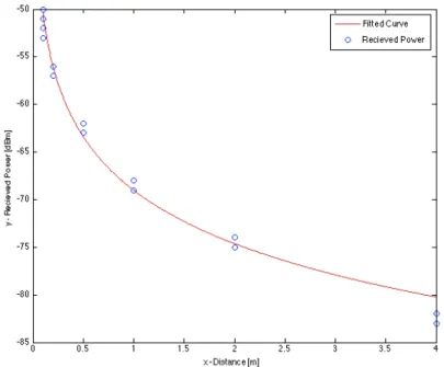
• The first experiment was done in outdoor environment in order to find ! value (power decay factor) in outdoor environment. To compute this value, a fixed anchor and a mobile device was used and they were placed at different distances from each other (10cm, 20cm, 50cm, 1m, 2m, 4m) in

(38)

Line-Of-Sight (LOS) conditions. For each condition the RSSI recording lasted for 200 seconds to have a reliable sample. After gathering the data to estimate the exponent we computed an exponential fitting, with the model:

!"#$%(!) = !_!− 10! log _!!

! (16)

The resulting value was ! = 1.865 as visible from Figure 8.

Figure 8: Fitted Curve based on outdoor experiment

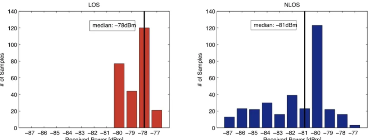
• The second experiment aim was finding the wall attenuation factor in our environment. To test the contribution of walls a couple of devices, emitting at -15dBm, was placed at 1m distance, in Line-Of-Sight (LOS) conditions or separated by a wall. In any condition the alignment of devices was the same, in order to maintain the same antenna coupling. Given the wall thickness of 0.1m, a LOS and six different NLOS (Not LOS) conditions (see Table 1) trials were recorded [1], with 1Hz sampling frequency, each lasting approximately 1 minute.

(39)

Trial ID Place Device A Device B 1 A 0m 0.9m 2 A 0.3m 0.6m 3 A 0.45m 0.45m 4 B 0m 0.9m 5 B 0.3m 0.60m 6 B 0.45m 0.45m

Table 1: Distances between Wall and devices for NLOS tests

As expected results depicted in Figure 9, show a significant reduction of RSSI, due to wall absorption. To compute the wall absorption we considered the shift of the median value: the LOS condition has a median of -78dBm, while the NLOS has a median of -81dBm. This means the Wall attenuation factor in our environment is 3dBm. As visible, the results show that there is a high variability in the received signal strength due to environment.

Figure 9: Histograms for LOS-NLOS comparison. As visible, the RSSI in NLOS conditions have a median shifted by -3dBm.

(40)

LAURA Quantities Estimation

The only quantities which are necessary to compute, for using LAURA method are the minimum distance between two devices (Self Distance) and the received power at minimum distance (Self Power). In order to find these values we carried out a simple experiment by putting two devices on top of each other and recording the data for three minutes [1]. The results:

Self Power -30mdB

Self Distance 0.04m

Table 2: Self Power and Self Distance values

Experiments

In this section the experiment procedure and materials for localization evaluating of LAURA and MWM methods are presented. The LAURA system relies on a sensor network based on the IEEE 802.15.4 standard, composed of:

1. anchor nodes, which are part of the infrastructure and are statically deployed in the areas to be monitored, built on MicaZ devices; 2. client nodes, attached to patients in order to support localization,

tracking, and patient supervision services, built on Shimmer devices.

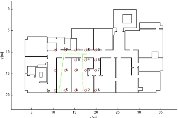
We carried out two acquisitions in two different days. We will call the stored result of these two acquisitions as Dataset A and Dataset B. The acquisitions have been carried on by deploying 18 fixed anchors on second floor of department building. The map of the building and the fixed anchor locations are shown in Figure 10.

(41)

Figure 10: Map of the building, fixed devices are shown with blue circles.

Not all the anchors were reachable along the whole acquisition, due to normal signal changes and dynamic network reshaping. The system parameters adopted [1] are listed in the Table 3:

Parameter Value ZigBee Channel 26 Transmission Pw -3mdB F. Sampling 1Hz Beaconing period 200ms Self Power -30mdB Self Distance 0.04m

Table 3: System Parameters

The mobile device was worn by a tester, walking inside the building, following a predefined path for each acquisition. The subject was moving in a real world environment, with other people in the building normally doing their activities. The recordings comprises the following:

(42)

RSSI: The RSSI values received from each fixed or mobile device, coupled with the timestamp related;

D: The sub-matrix of the distances between the anchors;

S: The sub-matrix of the RSSI values among the anchors which reach the mobile device;

pos: The real position of the mobile device at each timestamp;

Having gathered all these data, it was possible to run LAURA, and Multi Wall Model (MWM) methods offline separately, obtaining:

!: The estimated distances to the reachable anchors;

!"#$: The estimated position of the mobile target after the multilateration; The multilateration method used in this study is grid-based lateration.

Results

In this section the results obtaining by running offline both Methods (LAURA and MWM) for both Datasets are presented separately.

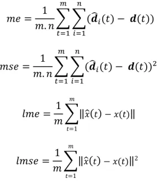
To evaluate the methods performances we used two couples of indicators: the mean error (me) and mean square error (mse) over distance estimation; localization mean error (lme) and localization mean square error (lmse).

If ! shows the number of samples and ! shows the number of fixed anchors; and ! is the estimated distance of mobile node from each anchor node, ! is the real distance of mobile node from each anchor node, ! is the estimated position, ! is the real position; then we can define the formula for calculating these errors as:

(43)

!" =

1 !. !

(!

!

(!) − !(!)

! !!! ! !!!

)

(17)

!"# =

1 !. !

(!

!

(!) − !(!))

! ! !!! ! !!!

(18)

!"# =

1 !

! ! − !(!)

(19) ! !=1

!"#$ =

1 !

! ! − !(!) 2 ! !=1

(20)

The squared version always penalizes larger errors more.

Table 4 presents the errors for LAURA and MWM separately in Dataset A:

me mse lme lmse

LAURA 0.5916 2.1580 1.6418 3.5400

MWM 0.4785 1.4092 1.9571 4.5914

Table 4: Errors of LAURA and MWM methods for Dataset A

And the errors for Dataset B are shown in Table 5:

me mse lme lmse

LAURA 0.5412 1.9701 1.7050 3.9550

MWM 0.5310 1.7113 2.1734 6.5804

Table 5: Errors of LAURA and MWM methods for Dataset B

As we can see from the two tables the mean and mean square error for MWM is smaller than LAURA method, but localization mean error and localization mean square error for LAURA is better than MWM. This means that the MWM method works better in estimation distance between mobile node and each anchor node, but after multilateration, the final estimated position in LAURA is more accurate.

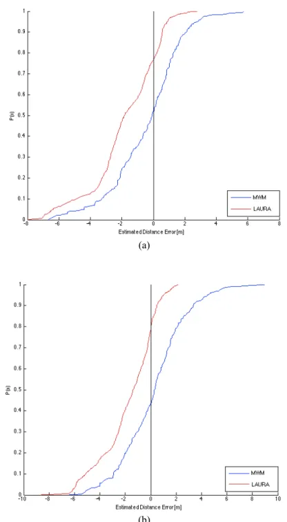
In order to compare the performance of methods before and after lateration, empirical cumulative distribution function (ecdf) graphs for both datasets before

(44)

lateration and after lateration are presented. Figure 11 depicts ecdf graphs of error before lateration for Dataset A and Dataset B respectively.

(a)

(b)

Figure 11: ecdf graphs of estimated distance error before lateration. (a) Dataset A, (b) Dataset B

As we can see in the graphs, in both datasets the LAURA line shifted toward the negative side of the x-axis, which means that LAURA algorithm underestimate the

(45)

distance position. MWM line is almost symmetric around zero, meaning the distance estimation is less biased. A further prove with respect to the me and mse for MWM method in both datasets.

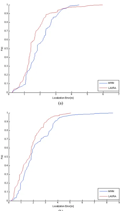
Figure 12 depicts ecdf graphs of error after lateration for Dataset A and Dataset B respectively.

(a)

(b)

(46)

As we can see in the graphs, in both datasets the LAURA line is over the MWM line and it is closer to the value 1 of y-axis. This means LAURA has a better estimation position after lateration. The same conclusion can be drawn based on the results of lme and lmse for LAURA method, as reported in Table 4, 5. Since one method has a lower error before lateration and the other one has lower error after lateration, by mixing them we might achieve better results.

In next section we define mixture methods in order to exploit the different behavior of the methods and improve position estimation.

(47)

Chapter 4 Accuracy-driven Mixture Method for

IHL Systems

Introduction

Based on the fact that MWM has a better estimation before lateration and LAURA method has better performance after lateration, it can be advantageous to mix these two algorithms to find an improvement of position estimation.

First of all, before explaining the methods, let us to define variables that are used in this section:

As already mentioned S is a vector of size n (n is the number anchor nodes) that shows the strength of received signal at the mobile node, emitted by each anchor node:

! = [!_!, !_!, … , !_!] (21) The next variable is ! which is a vector of size n that shows the estimated distance of mobile node from each anchor node:

(48)

The other quantity would be ! which is again a vector of size n that shows the distance between estimated position after lateration and each anchor node.

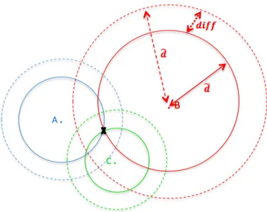
! = [! _!, ! _!, … , ! _!] (23) ! _!= !"#$%&#!'()"$#$)* − !"#_! (24) The last variable defined in this part is diff which is a vector computed by subtraction of ! and !, actually showing the shift between the distances to each anchors as estimated on signals and after lateration.

!"## = ! − ! (25)

Figure 13 illustrates a graphical definition of variables. The blue x sign is estimated position of mobile node.

(49)

Basic Methods

In order to improve the precision of position estimation, we implemented three methods, using a static mixture policy. The recorded signals were employed to compute the target position, comparing the results in order to identify improvements.

In the first approach we used all the distances estimation together (merging ! from LAURA and MWM) and minimized the overall error to perform multilateration. Employing also the more precise estimations by MWM, we possibly improve the overall results.

Table 6 shows the error result we get from Dataset A, B after multilateration:

lme lmse

Dataset A 1.6113 3.3842

Dataset B 1.7006 3.9156

Table 6: Localization Error of the first basic mixture method.

(50)

(b)

Figure 14: ecdf of localization error for the first basic mixture method. (a) Dataset A, (b) Dataset B

If we compare this result with the Tables 4, 5 we can notice a very slight improvement for both datasets. The localization error of the merged method is giving us a better result than LAURA, but this improvement is so limited it might not be significant. Figure 14 depicts the ecdf of localization estimation error for Dataset A and B.

The second approach we implemented was exploiting the average of the estimated distances of LAURA and MWM algorithms. After computing the position after multilateration, new estimated positions were obtained and the estimation error was calculated for this approach.

lme lmse

Dataset A 2.5032 7.6402

Dataset B 2.5460 8.0187

(51)

By comparing the error of this approach with raw MWM and LAURA errors, we can see there is no improvement, while the error is worse than both MWM and LAURA methods for both datasets.

Figure 15 depicts the ecdf of localization estimation error for Dataset A and B.

(a)

(b)

Figure 15: ecdf of localization error for the second basic mixture method. (a) Dataset A, (b) Dataset B

(52)

The last approach is to compute the average of the position estimated after lateration for MWM and LAURA separately. As before we calculate the error for new estimated position.

lme lmse

Dataset A 1.6930 3.4474

Dataset B 1.8788 4.6154

Table 8: Localization Error of the third basic mixture method.

By analyzing the result we see that localization error for the average estimation is better than MWM only, while LAURA has still a better estimation.

Figure 16 depicts the ecdf of localization estimation error for Dataset A and B.

(53)

(b)

Figure 16: ecdf of localization error for the third basic mixture method. (a) Dataset A, (b) Dataset B

Estimation Confidence Indicators

In previous part the basic mixture methods of LAURA and MWM were presented, yet we did not obtain a considerable improvement.

Since we have the estimation position for both LAURA and MWM, the idea is if in each time instant we can select the estimation position of the method with lower error then we can reduce the localization error. Having no information about estimation error at runtime means it is not possible to know which algorithm has a better position estimation; we thus introduce some indictors to improve the mixture policy by predicting which is the best method at each time instant.

(54)

1. Shift Root Mean Square (RMS): also known as the quadratic mean, is a statistical measure of the magnitude of a varying quantity. In our study RMS is defined as:

!"# = 1_! diff ! ! !

!!!

(26)

Bigger RMS means that a bigger overall shift is introduced while lateration. The fact that summation terms are squared contributes to penalize situations with greater shifts. In ideal conditions this shift is null since ! is equal to ! is affected by errors.

2. Shift Variance: Variance measures how far a set of numbers is spread out.

In our study Shift Variance is defined as below:

!"# = 1

! diff !− !"#$ diff ! !

!

!!!

(27)

Variance is always non-negative: small values indicates that the shifts diff tends to be very close to their mean (expected value) and hence to each other, while a high variance indicates that the shifts are very spread out around the mean and far from each other. In particular this indicator neglects shifts shared by all the anchors distances, highlighting inhomogeneities only. Again in ideal conditions diff is null, but in this case the indicator remains null as long as the error on ! is the same for all the anchors.

3. Sum of Variances (SumVar): It represents how much the last 5 estimated positions are spread out. At each time instant we make a window of the

(55)

estimated positions for the last 5 time instants. The formula for SumVar is as below:

estPos = [x, y]

w(t) = [x(t-4), x(t-3), x(t-2), x(t-1), x(t) ; y(t-4), y(t-3), y(t-2), y(t-1), y(t)]

!"#$%&(!) = !"#(!!(!)) − !"#(!!(!)) !

!!!

(28)

As it is shown in the formula SumVar at time t is computed by the sum of variance of x values and y values in window w(t). If SumVar is a small value it means that the mobile node estimated position has not changed considerably in the last 5 seconds; In ideal conditions this has a not-null value only when the target is moving. Nonetheless even in that situation the confidence is lower, due to delays and computation times.

4. Minimum Estimated Distance (MED): This indicator is defined as below: !"# = min_!!!…! d _! (29) MED shows the minimum distance estimated between the mobile node and the available anchor nodes. Indeed if the target is closer to an anchor it is less probable that walls or obstacles affect the signal, resulting in a more confident estimation.

After defining 4 indicators, the next section identifies the correlation between defined indicators and positioning estimation error by carrying on experiments and computing their correlations on these experiments.

(56)

Experimental Data

Since we carried out two acquisitions and we simulated two methods (LAURA and MWM) on each dataset, at the end we had 4 different results separately. We analyze these results and compute the correlation between our defined indicators in previous section and positioning estimation error (error). We calculated all the indicators for datasets A and B with both LAURA and MWM methods. The following graphs in figures 17, 18, 19, 20 show indicators behavior.

(57)

Figure 17: The error value and each indicator value for LAURA method in Dataset A are shown separately. The red line in all the graphs shows error value.

After providing all the graphs, in order to understand the relation between error and indicators, the correlation between error and each indicator were calculated. The result is shown in Table 9:

RMS Variance SumVar MED Error 0.0237 0.0396 0.3399 0.4232

Table 9: Correlation value between error and indicators in dataset A in LAURA method

For LAURA method in Dataset A the correlation for RMS and Variance is very low and it shows there is no significant relation for these indicators and error. For two other indicators (SumVar and MED) and especially for SumVar the correlation is considerable.

(58)

Figure 18: The error value and each indicator value for MWM method in Dataset A are shown separately. The red line in all the graphs shows error value.

(59)

After providing all the graphs, in order to understand the relation between error and indicators, the correlation between error and each indicator were calculated. The result is shown in Table 10:

RMS Variance SumVar MED Error -0.1336 -0.241 0.2850 0.5351

Table 10: Correlation value between error and indicators in dataset A in MWM method

By Analyzing the data in Table 10 for MWM method in Dataset A it is visible that the correlation for RMS and Variance are negative numbers, it means that the error is introduced as the estimated position is limited avoiding wall-crossing. Correlation value for SumVar is 0.2850, it is not good enough but works better that the other two indicators, and the best indicator is MED which has a good correlation value of 0.5351.

The third set of graphs that are shown in Figure 19 are the result of LAURA method for Dataset B:

(60)

Figure 19: The error value and each indicator value for LAURA method in Dataset B are shown separately. The red line in all the graphs shows error value.

The correlation between error and each indicator showed the results in Table 11:

(61)

By analyzing the table it is visible that correlation value for RMS and Variance are negative again as it was in the previous case. We can notice that SumVar is second best indicator with value of 0.2354, and MED indicator has best correlation value among 4 indicators by value of 0.4220.

The last set of graphs that are shown in Figure 20 are the result of MWM method for Dataset B:

(62)

Figure 20: The error value and each indicator value for MWM method in Dataset B are shown separately. The red line in all the graphs shows error value.

The correlation between error and each indicator showed the results in Table 12:

Table 12: Correlation value between error and indicators in dataset B in MWM method

By analyzing the table it is visible that correlation value for RMS and Variance are negative again as it was in the previous cases. We can notice an improvement of correlation value for SumVar and MED in MWM method of Dataset B. SumVar is second best indicator with value of 0.4948 and is almost 0.5 which is a good correlation value, and MED indicator has the best correlation value among 4 indicators by value of 0.6660 and has a significant value.

By calculating the four indicators in four different samples and algorithms we could conclude that RMS and Variance didn’t have expected impact to estimation error and we cannot use these two indicators. Nonetheless SumVar and MED indicators had a significant result and correlation with estimation error, so we decided to choose these two indicators to keep on our analyses.

(63)

Mixture Methods based on Estimation Confidence Indicators

As it was explained before, based on correlation value, SumVar and MED had significant correlation with estimation error and we choose these two indicators to use for mixture methods. The chosen policy relies on the indicators as follow:

!: !" !"# !, !"#1 < !"# !, !"#2 → !""#" !, !"#1 < !""#"(!, !"#2) This means that for better estimations of algorithm 1 the indicator for algorithm 1 has to be lower than the algorithm 2.

To check if this hypothesis is correct we need to compute Accuracy and Precision of this relation for each indicator, and also build ROC space for each indicator. The Accuracy of a measurement system is the degree of closeness of measurements of a quantity to that quantity's actual (true) value. The precision of a measurement system, related to reproducibility and repeatability, is the degree to which repeated measurements under unchanged conditions show the same results.

To obtain the Accuracy and Precision values, first we need to define following four variables in our study:

True Positive (TP): !"# !, !"#$" < !"# !, !"! && !""#" !, !"#$" < !""#"(!, !"!) True Negative (TN): !"# !, !"! < !"# !, !"#$" && !""#" !, !"! < !""#"(!, !"#$") False Positive (FP): !"# !, !"#$" < !"# !, !"! && !""#" !, !"#$" > !""#"(!, !"!) False Negative (FN): !"# !, !"! < !"# !, !"#$" && !""#" !, !"! > !""#"(!, !"#$") Having these definitions, Accuracy and Precision are computed as:

Accuracy driven hybrid localization method

POLITECNICO DI MILANO

Scuola di Ingegneria dell’Informazione

POLO TERRITORIALE DI COMO

Master of Science in Computer Engineering

Accuracy-driven Hybrid Localization Method

Supervisor: Prof. Fabio Salice

Assistant Supervisor: Eng. Fabio Veronese

Master Graduation Thesis by: Majid Farzaneh

Student Id. Number: 780117

ABSTRACT

SOMMARIO

Table of

Contents

List of Figures

List of Tables

Glossary

Chapter 1

Introduction

Introduction

Structure of the Thesis

Chapter 2

Indoor Human Localization (IHL):

Radio-Frequency Based Technologies

and Methods

Problem Formulation

Distance Estimation Methods

Localization Methods

Physical Quantity Classification

Technology and Frequency Classification

Signal Propagation Models

Ray Tracing

One-Slope Model:

! ! = !

+ 10 ! log !

Multi-Wall Model

!

= !

! +

!

!

+ !

!

LAURA Propagation Model

! = ℱ ! !

!!

Chapter 3

Localization Methods Evaluation

MWM Quantities Estimation

LAURA Quantities Estimation

Experiments

Results

!" =

1

!. !

(!

(!) − !(!)

)

!"# =

1

!. !

(!

(!) − !(!))

!"# =

1

!

!"#$ =

1

!

Chapter 4

Accuracy-driven Mixture Method for

IHL Systems

Introduction

Basic Methods

Estimation Confidence Indicators

Experimental Data

Mixture Methods based on Estimation Confidence Indicators

_!!