A
Pred
Superv
Analys
dictive
visor: Prof
P
Scuol
Master o
sis and
e Con
f. Riccardo
OLITEC
la di Inge
of Science
d Imp
ntrol (M
o SCATTO
CNICO D
egneria de
e in Autom
lemen
MPC)
OLINI
DI MILAN
ell’Inform
mation E
ntation
) in Ch
MaANO
mazione
ngineerin
n of M
hemica
aster Gradu Shahab Rez Student Id.ng
Model
al Pla
uation Thesi za BESHA . number 76nt
is by: ARAT 64488Abstract
Model based Predictive Control (MPC) is a form of control that has gained widespread acceptance in chemical industry due to its unique advantages compared to classic control methods. The main distinguishing features are the ability to efficiently control large scale interconnected systems and the inherent ability to cope with physical and other constraints of the controlled system. MPC controllers are designed on the basis of a dynamical model of the system that has to be controlled (i.e., the plant) and apply mathematical optimization techniques in order to obtain the optimal inputs to be applied to the plant. MPC acquires the current control action by solving, at each sampling instant, a finite horizon open-loop optimal control problem, using the current state of the plant as the initial state; the optimization yields an optimal control sequence and the first control in this sequence is applied to the plant. In this thesis the focus is on linear MPC algorithms, i.e., MPC algorithms that can take the regulation problem. More specifically, the main aim of this thesis is the development of MPC algorithms in the environment of MATLAB and Simulink that can take input and output constraints into account and can guarantee stable behavior and acceptable performance. These aims are achieved by making improved algorithms for the construction of required matrixes and contributions to the constraints. On the level of stability, celebrated terminal state is enabled the pledge. We concentrate our attention on a plant with two reactors and a separator as a sample of chemical plant in order to enrich the experimental results. Several simulations on the model of this process show the improved properties of the obtained program.
Keywords:
Model predictive control; chemical plant; CSTR; optimal control; constraint; stability
Sommario
Il controllo predittivo, o MPC (Model Predictive Control) è una tecnica di sintesi di sistemi di controllo che ha riscosso un notevole successo nell’industria chimica per I vantaggi che può offrire rispetto a metodi classici, quali l’assegnamento degli autovalori o il controllo LQR. Le sue principali caratteristiche sono la possibilità di considerare sistemi con grandi dimensioni, tipicamente costituiti da sottosistemi interconnessi, a la capacità di tenere conto in modo esplicito di eventuali vincoli sulle variabili di processo o su altre variabili di interesse. I controllori MPC sono di tipo “model-based”, cioè sono progettati a partire da un modello del processo sotto controllo, e si basano sulla formulazione di un opportuno problema di ottimizzazione da risolversi a ogni istante di campionamento per determinare il valore da imporre alle variabili di controllo. Più nello specifico, viene risolto un problema di controllo su orizzonte finito dove lo stato corrente è considerato come stato iniziale. La soluzione del problema di ottimo consiste nel determinare la sequenza di controlli ottimi da imporre, almeno teoricamente, lungo tutto l’intervallo considerato. Tuttavia, si implementa effettivamente soltanto il primo valore di questa sequenza e l’intera procedura è ripetuta al successivo istante di campionamento. In questo lavoro di Tesi si sviluppano in ambiente Matlab/Simulink due algoritmi MPC per sistemi lineari e se ne analizzano in dettaglio le caratteristiche e prestazioni. Entrambi gli algoritmi consentono di considerare vincoli sullo stato, sulle variabili di controllo e sulle uscite regolate, così da garantire stabilità e prestazioni. Per quanto riguarda la stabilità, è possibile introdurre nel problema di ottimizzazione un opportuno peso sullo stato finale raggiunto dal sistema al termine dell’orizzonte di predizione, vincolandolo anche ad appartenere a un dato insieme. Le caratteristiche di questi metodi MPC sono confrontate con riferimento a un processo, costituito da due reattori e da un separatore, in grado di rappresentare bene le problematiche tipiche di un impianto industriale. Nel lavoro sono riportate e commentate numerose simulazioni che consentono di mostrare le prestazioni ottenibili con questo approccio alla sintesi del controllore.
Keywords:
Acknowledgments
This thesis presents the results of the study carried out in the means of graduation on Master of Science in Automation engineering at Politecnico di Milano under the supervision of Prof. Riccardo Scattolini.
I would like to address a special word of gratitude to Prof. Scattolini; without whom the subject gathered in this thesis would have not been possible. Throughout my studies he took an active interest in my work and encouraged me to keep at it when I couldn’t see the light at the end of the tunnel. I will always be grateful for his investment of patience, time and effort in my work.
I would also like to take this opportunity to thank Prof. Sergio Bittanti and Prof. Paolo Rocco for allowing me to contribute in the IFAC Milano 2011 as a volunteer student. It was one of my greatest academicals experience.
A special thanks goes to Prof. Franco Zappa for his entire support to international students during the first days of university life in Milano and in the course “Electronic System”, at any time.
I am grateful to Prof. Marco Lovera and Prof. Alberto Leva for their astonishing classes in “Advanced and Multivariable Control” and “Automation of Energy systems” which were sources of inspiration for me.
During the two years I have studied on my Master program, I had the opportunity to spend enjoyable moments in the company of friends and colleagues. I would like to thank all of them.
I am eternally indebted to my wife Hananeh for her endless love and support and our parents for all their best wishes.
This thesis is dedicated to my wife.
Shahab R. Besharat Milano, December, 2012
Contents
Abstract ... 1 Sommario ... 2 Acknowledgments ... 3 List of Figures ... 7 List of Tables ... 9 Notation ... 10 1 Introduction ... 12 1.1 Motivation ... 13 2 Dynamic model of chemical process ... 20 2.1 Introduction to process control ... 20 2.2 Process dynamic ... 20 2.3 Process control ... 21 2.4 The hierarchy of process control activities ... 24 2.4.1 Measurement and actuation (Level 1) ... 24 2.4.2 Safety and environmental/equipment protection (Level 2) ... 25 2.4.3 Regulatory control (Level 3a) ... 25 2.4.4 Multivariable and constraint control (Level 3b) ... 25 2.4.5 Real‐time optimization (Level 4) ... 26 2.4.6 Planning and scheduling (Level 5) ... 27 2.5 Continuous stirred tank reactor models ... 29 2.5.1 The mass balance ... 29 2.5.2 The component balance ... 30 2.5.3 Adding a chemical reaction to the stirred tank model ... 31 2.5.4 The energy balance ... 32 2.6 Case object ... 34 3 Model Predictive Control ... 39 3.1 Historical issues on MPC in process control ... 433.3 Closed‐loop _ open‐loop analysis ... 50 3.3.1 IH‐LQ ... 50 3.3.2 FH optimal control ... 51 3.3.3 RH problem ... 54 3.4 MPC formulation without integral action ... 57 3.5 MPC formulation with integral action ... 61 3.6 Extension to the basic formulation ... 65 4 Stability ... 66 4.1 Stability analysis ... 66 4.1.1 Definitions ... 67 4.1.2 RH and IH‐LQ control... 69 4.2 Stabilizing modifications ... 71 4.2.1 Constrained IH‐LQ control ... 71 4.3 Achievements on MPC stability ... 75 5 Simulation in MATLAB and Simulink ... 76 5.1 Model of the system ... 76 5.2 Linearization ... 76 5.3 Required matrix construction ... 81 5.4 Optimization by Quadprog ... 83 5.4.1 Optimization for controller without Integral action ... 83 5.4.2 Optimization for controller with Integral action ... 84 5.5 Constraints ... 86 5.6 Controller design ... 88 5.6.1 Controller without integral action ... 88 5.6.2 Controller with integral action ... 90 6 Experimental results ... 92 6.1 Results for the MPC controller without integral action ... 93 6.1.1 Simulation 1: tuning the level of first reactor ... 93
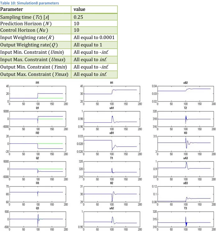
6.1.2 Simulation 2: input weighting effect ... 98 6.1.3 Simulation 3: output weighting effect ... 100 6.1.4 Simulation 4: prediction and control horizons ... 102 6.1.5 Simulation 5: disturbance effect ... 103 6.1.6 Simulation 6: input constraint ... 105 6.1.7 Simulation 7: output constraint ... 106 6.1.8 Conclusion on MPC controller without integral action ... 108 6.2 Results for MPC controller with integral action ... 109 6.2.1 Simulation 8: tuning the level of first reactor ... 109 6.2.2 Simulation 9: input weighting effect ... 114 6.2.3 Simulation 10: output weighting effect ... 116 6.2.4 Simulation 11: prediction and control horizons ... 117 6.2.5 Simulation 12: disturbance effect ... 119 6.2.6 Simulation 13: input constraint ... 120 6.2.7 Simulation 14: output constraint ... 121 6.2.8 Conclusion on MPC controller with integral action ... 123 Appendix A ... 125 A.1 MATLAB codes of first subsystem model ... 125 A.2 MATLAB codes for preparation of MPC parameters without integral action ... 126 A.3 MATLAB codes for construction of matrixes without integral action ... 126 A.4 MATLAB codes for MPC function without integral action ... 129 A.5 MATLAB codes for preparation of MPC parameters with integral action ... 129 A.6 MATLAB codes for construction of matrixes with integral action ... 130 A.7 MATLAB codes for MPC function with integral action ... 132 Bibliography ... 133
List of Figures
Figure 1: Participants of APC survey by industry and by continent ... 17 Figure 2: Industrial use of APC methods ... 17 Figure 3: Hierarchy of process control activities ... 28 Figure 4: Mixed Tank of Liquid ... 30 Figure 5: CSTR with cooling coil removing energy (Q) ... 32 Figure 6: Two reactors in series with separator and recycle ... 35 Figure 7: Receding horizon scheme ... 54 Figure 8‐1: Plugging the integral action ... 63 Figure 8‐2: disappearing the integrator in augmented state block diagram ... 63 Figure 9: Integral action in augmented state block diagram ... 64 Figure 10: stabilized sets in the RH and IH‐LQ unconstrained control ... 70 Figure 11: Stabilized sets in the constrained IH‐LQ control ... 73 Figure 12: Simulate the model with MATLAB function ... 78 Figure 13: the Model of fist reactor ... 78 Figure 14: intermediate scheme for first reactor model ... 79 Figure 15: Control diagram of MPC without integral action ... 88 Figure 16: MPC controller without integral action in Simulink ... 89 Figure 17: Control diagram of MPC with integral action ... 90 Figure 18: MPC controller with integral action in Simulink ... 91 Figure 19: Result of H1 setpoint change in the system... 94 Figure 20: Result of H1 setpoint change in the system‐zoomed ... 95 Figure 21: Response of H1 to the setpont change ... 96 Figure 22: Result of H1 setpoint change in Ff1, Ff2, H1 and H2 (normalized) ... 97 Figure 23: Result of input weighting with H1 setpoint change in Ff1, Ff2, H1 and H2 (normalized)99 Figure 24: Result of output weighting with H1 setpoint change in Ff1, Ff2, H1 and H2 (normalized) ... 101 Figure 25: Result of horizons with H1 setpoint change in Ff1, Ff2, H1 and H2 (normalized) ... 103 Figure 26: Result of disturbance in the system ... 104 Figure 27: Result of constraint for Ff1 with H1 setpoint change ... 106 Figure 28: Result of constraint for T1 with H1 setpoint change ... 107 Figure 29: Result of H1 setpoint change in the system with integrator ... 110 Figure 30: Result of H1 setpoint change in the system with integrator‐zoomed ... 111 Figure 31: Response of H1 to the setpoint change with integrator ... 112 Figure 32: Result of H1 setpoint change in Ff1, Ff2, H1 and H2 (normalized) with integrator ... 113 Figure 33: Result of input weighting with H1 setpoint change in Ff1, Ff2, H1 and H2 (normalized) with integrator ... 115Figure 34: Result of output weighting with H1 setpoint change in Ff1, Ff2, H1 and H2 (normalized)
with integrator ... 117
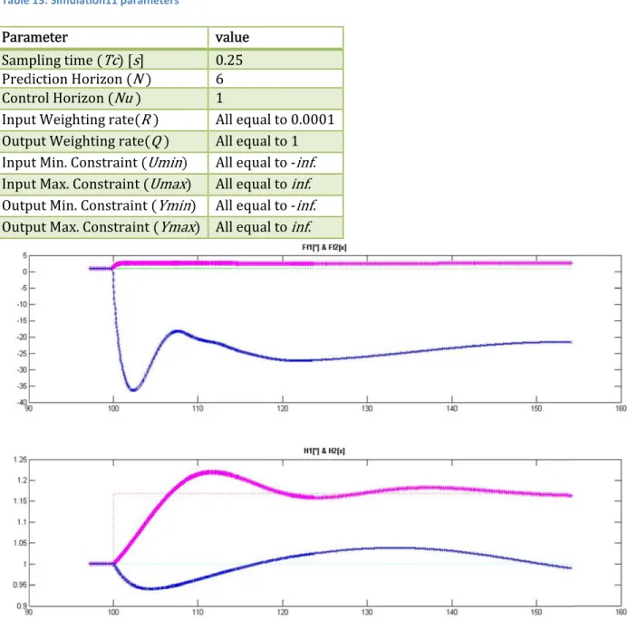
Figure 35: Result of horizons with H1 setpoint change in Ff1, Ff2, H1 and H2 (normalized) with integrator ... 118 Figure 36: Result of disturbance in the system with integrator ... 119 Figure 37: Result of constraint for dFf1 with H1 setpoint change with integrator ... 121 Figure 38: Result of constraint for H2 with H1 setpoint change with integrator ... 122
List of Tables
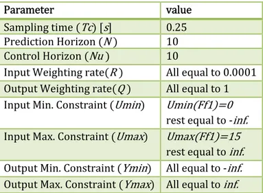
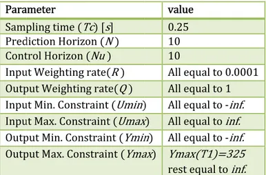
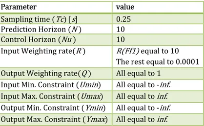
Table 1: Summary of linear MPC applications by areas ... 14 Table 2: Summary of NMPC applications by areas ... 16 Table 3: Steady state and parameters ... 37 Table 4: Simulation1 parameters ... 93 Table 5: Simulation2 parameters ... 98 Table 6: Simulation3 parameters ... 100 Table 7: Simulation4 parameters ... 102 Table 8: Simulation6 parameters ... 105 Table 9: Simulation7 parameters ... 107 Table 10: Simulation8 parameters ... 110 Table 11: Simulation9 parameters ... 114 Table 12: Simulation10 parameters ... 116 Table 13: Simulation11 parameters ... 118 Table 14: Simulation13 parameters ... 120 Table 15: Simulation14 parameters ... 122Notation
a, b, c ∈ Lower case roman symbols denote scalar or vector variables A, B, C ∈ Upper case roman symbols denote matrix variables
, ∈ Upper case Unicode extended characters denote augmented matrices
, Set of real numbers and positive real numbers
≔ Assignment
a ≔ b ⇔ the value of b is assigned to variable a , (Strict) scalar inequality
a > b ⇔ a − b has strictly positive elements
, (Strict) matrix inequality
A > 0 ⇔ A is strictly positive definite
∈ m-dimensional input vector at discrete time k
∈ n-dimensional state vector at discrete time k
∈ p-dimensional output vector at discrete time k
∈ d-dimensional disturbance vector at discrete time k
, ̅, Steady state values for inputs, states and outputs Reference values for outputs or setpoint
Prediction horizon length Control horizon length , Transpose of matrix A
‖ ‖ Weighted 2-norm of a vector: ′ Function minimization over x,
optimal function value is returned
Motto:
“There is nothing more
practical than a good theory.”
-Boltzmann
1 Introduction
In this age of globalization, the realization of production innovation and highly stable operation is the chief objective of the process industry. Obviously, modern advanced control plays an important role to achieve this target, but the key to success is the maximum utilization of PID control and conventional advanced control. It is obvious that the three central pillars of process control – PID control, conventional advanced control, and linear/nonlinear model predictive control – have been widely used and they have to be contributed toward increasing productivity.
Model predictive control (MPC) or receding horizon control (RHC) is a form of control in which the current control action is obtained by solving on-line, at each sampling instant, a finite horizon open-loop optimal control problem, using the current state of the plant as the initial state; the optimization yields an optimal control sequence and the first control in this sequence is applied to the plant. This is its main difference from conventional control which uses a pre-computed control law.
Model predictive control is one of few suitable methods, and this fact makes it an important tool for the control engineer, particularly in the process industries where plants being controlled are sufficiently slow to permit its implementation. Other
include unconstrained nonlinear plants, for which on-line computation of a control law usually requires the plant dynamics to possess a special structure, and time-varying plants.
1.1 Motivation
This thesis aims to reveal the principal of model predictive control, its formulation, historical issues and some practical tricks. Finally, by implementing this theory in a typical chemical process, as a plant consisting of two reactors and a separator in the Simulink environment, try to represent the advantages of this state of the art method. To motivate the idea of using MPC control, here are some fact according to the international surveys and researches.
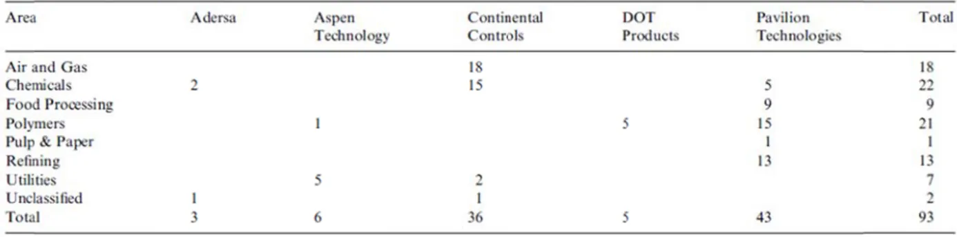
The first fact is coming from the article “A survey of industrial model predictive control technology” by Quin and Badgwell (2003). According to their research, in Tables 1 and 2, where more than 4600 total MPC applications are reported, MPC technology can now be found in a wide variety of application areas. The largest single block of applications is in refining, which amounts to 67% of all classified applications. This is also one of the original application areas where MPC technology has a solid track record of success. A significant number of applications can also be found in petrochemicals and chemicals, although it has taken longer for MPC technology to break into these areas.
Sign aero Table Tab refin and the othe (pre nificant grow ospace and 1: Summary of le 1 shows ning and pe Invensys a food proce ers. The ap edictive func wth areas d automotive linear MPC app s that Aspe etrochemica apparently essing, mini pplications r ctional cont include the e industries plications by are enTech an als, with a had a bro ing/metallu reported by trol) applica e chemicals s. as d Honeywe handful of ader range rgy, aerosp y Adersa in ations, so it s, pulp and ell Hi-Spec application e of experie pace and a nclude a nu t is difficult paper, foo c were high ns in other ence with a automotive umber of em to report th od process hly focused areas. Ade applications areas, amo mbedded P heir numbe ing, d in ersa s in ong PFC r or
number of in-house SMOC (Shell multivariable optimizing controller) applications by Shell, so the distribution is likely to be shifted towards refining and petrochemical applications.
The bottom of Table 1 lists the largest linear MPC applications to date by each vendor, in the form of (outputs)_(inputs). The numbers show a difference in philosophy that is a matter of some controversy.
AspenTech prefers to solve a large control problem with a single controller application whenever possible; they report an olefins application with 603 outputs and 283 inputs. Other vendors prefer to break the problem up into meaningful sub-processes.
The nonlinear MPC (NMPC) applications reported in Table 2 are spread more evenly among a number of applications areas. Areas with the largest number of reported NMPC applications include chemicals, polymers, and air and gas processing. It has been observed that the size and scope of NMPC applications are typically much smaller than that of linear MPC applications. This is likely due to the computational complexity of NMPC algorithms.
Table In a proc justi (APC term fram part indu 2: Summary of another wor cess contro fy the cost C) technolo ms and tha mework for icipants of ustrial use o NMPC applicati rk by Baue ol-A survey t associated ogies to a at paper the econo APC surve of APC met ions by areas r and Craig y and frame d with the process, th reviews th omic evalu ey by indust hods. g (2007) “E ework” it h introduction he benefits hese metho uation of A trial and by Economic a has been in n of new a have to be ods and i APC projec y continent a assessmen ndicated th dvanced p e quantified incorporate cts. Figure and Figure nt of advanc hat In order rocess con d in econo es them in 1 shows 2 is about ced r to ntrol mic n a the the
Fina in th cont MPC past ally to conc he Journal trol in Japa C, releases t, because Figure 1: P lude about of Proces an” is going s operators the optim Participants of A Figure 2: Ind this motiva s Control a to be refer from most al operatin APC survey by in ustrial use of AP ation, recen as “The sta rred. It has t of the adju ng conditio ndustry and by c PC methods nt paper of ate of the s been note ustment wo n is autom continent Kanu and O art in che ed that imp ork they ha matically de Ogawa (20 mical proc lementation ad to do in etermined a 010) ess n of the and
maintained under disturbances. In addition, MPC makes it possible to maximize production rate by making the most use of the capability of the process and to minimize cost through energy conservation by moving the operating condition toward the control limit. Both the energy conservation and the productive capacity were improved by an average of 3 to 5% as the result of APC projects centered on MPC at Mitsubishi Chemical Corporation (MCC).
At the end of that paper, the MPC application for energy conservation and production maximization of the olefin unit at MCCMizushima plant is briefly explained which is the largest MPC application in the world, consisting of 283 manipulated variables and 603 controlled variables. The subsequent two commentaries are appreciated to declaim.
A skilled operator made the following comment on this MPC application: “We had operated the Ethylene fractionator in constant pressure mode for more than 20 years. I was speechless with surprise that we had made an enormous loss for many years, when I watched the MPC decreased the column pressure, improved the distillation efficiency, and maximized the production rate.” Another process control engineer said “I had misunderstood that setpoints were determined by operation section and process control section took the responsibility only for control. I realized MPC for the first time; it makes the most use of the capability of
equipments, determines setpoints for economical operation, and maintains both controlled variables and manipulated variables close to the setpoints.”
2 Dynamic model of chemical process
2.1 Introduction to process controlIn recent years the performance requirements for process plants have become increasingly difficult to satisfy. Stronger competition, tougher environmental and safety regulations, and rapidly changing economic conditions have been key factors in tightening product quality specifications. A further complication is that modern plants have become more difficult to operate because of the trend toward complex and highly integrated processes. For such plants, it is difficult to prevent disturbances from propagating from one unit to other interconnected units.
In view of the increased emphasis placed on safe, efficient plant operation, it is only natural that the subject of process control has become increasingly important in recent years. Without computer-based process control systems it would be impossible to operate modern plants safely and profitably while satisfying product quality and environmental requirements. Thus, it is important for Automation engineers to have an overview about the process control.
2.2 Process dynamic
The term process dynamics refers to unsteady-state (or transient) process behavior. By contrast, most of the engineering may emphasize steady-state and equilibrium conditions in subjects as material and energy balances,
important. Transient operation occurs during important situations such as start-ups and shutdowns, unusual process disturbances, and planned transitions from one product grade to another.
2.3 Process control
The primary objective of process control is to maintain a process at the desired operating conditions, safely and efficiently, while satisfying environmental and product quality requirements. The subject of process control is concerned with how to achieve these goals. In large-scale, integrated processing plants such as oil refineries or ethylene plants, thousands of process variables such as compositions, temperatures, and pressures are measured and must be controlled. Fortunately, large numbers of process variables (mainly flow rates) can usually be manipulated for this purpose. Feedback control systems compare measurements with their desired values and then adjust the manipulated variables accordingly.
The foundation of process control is process understanding. Thus, we continue with a basic question-What is a process? For our purposes, a brief definition is appropriate:
Process: The conversion of feed materials to products using chemical and physical operations. In practice, the term process tends to be used for both the processing operation and the processing equipment.
Note that this definition applies to three types of common processes: continuous, batch, and semibatch.
Following, we consider representative of continuous processes which is a main subject of this thesis. Here briefly summarize key control issues.
The process control problem has been characterized by identifying three important types of process variables.
• Controlled variables (CVs): The process variables that are controlled. The desired value of a controlled variable is referred to as its set point.
• Manipulated variables (MVs): The process-Variables that can be adjusted in order to keep the controlled variables at or near their set points. Typically, the manipulated variables are flow rates.
• Disturbance variables (DVs): Process variables that affect the controlled variables but cannot be manipulated. Disturbances generally are related to changes in the operating environment of the process, for example, its feed conditions or ambient temperature. Some disturbance variables can be measured on-line, but many cannot.
The specification of CVs, MVs, and DVs is a critical step in developing a control system. The selections should be based on process knowledge, experience, and control objectives.
2.4 The hierarchy of process control activities
As mentioned earlier, the chief objective of process control is to maintain a process at the desired operating conditions, safely and efficiently, while satisfying environmental and product quality requirements.
If we emphasized one process control activity and try to keeping controlled variables at specified set points, there are other important activities, also that we will now briefly describe.
In Fig.3 the process control activities are organized in the form of a hierarchy with required functions at the lower levels and desirable, but optional, functions at the higher levels. The time scale for each activity is shown on the left side of Fig.3. Note that the frequency of execution is much lower for the higher-level functions.
2.4.1 Measurement and actuation (Level 1)
Measurement devices (sensors and transmitters) and actuation equipment (for example, control valves) are used to measure process variables and implement the calculated control actions. These devices are interfaced to the control system. Clearly, the measurement and actuation functions are an indispensable part of any control system.
2.4.2 Safety and environmental/equipment protection (Level 2)
The Level 2 functions play a critical role by ensuring that the process is operating safely and satisfies environmental regulations. Generally, process safety relies on the principle of multiple protection layers that involve groupings of equipment and human actions. One layer includes process control functions, such as alarm management during abnormal situations, and safety instrumented systems for emergency shutdowns. The safety equipment operates independently of the regular instrumentation used for regulatory control in Level 3a.
2.4.3 Regulatory control (Level 3a)
As mentioned earlier, successful operation of a process requires that key process variables such as flow rates, temperatures, pressures, and compositions be operated at, or close to, their set points. This Level 3a activity, regulatory control, is achieved by applying standard feedback and feedforward control techniques. If the standard control techniques are not satisfactory, a variety of advanced control techniques are available.
2.4.4 Multivariable and constraint control (Level 3b)
Many difficult process control problems have two distinguishing characteristics: (i) significant interactions occur among key process variables, and (ii) inequality constraints exist for manipulated and controlled variables. The inequality
constraints include upper and lower limits. Limits on controlled variables reflect equipment constraints and the operating objectives for the process.
The ability to operate a process close to a limiting constraint is an important objective for advanced process control. For many industrial processes, the optimum operating condition occurs at a constraint limit. For these situations, the set point should not be the constraint value because a process disturbance could force the controlled variable beyond the limit. Thus, the set point should be set conservatively, based on the ability of the control system to reduce the effects of disturbances.
The standard process control techniques of Level 3a may not be adequate for difficult control problems that have serious process interactions and inequality constraints. For these situations, the advanced control techniques of Level 3b, multivariable control and constraint control, should be considered. In particular, the model predictive control (MPC) strategy was developed to deal with both process interactions and inequality constraints. MPC is the main subject of this thesis report.
2.4.5 Real‐time optimization (Level 4)
The optimum operating conditions for a plant are determined as part of the process design. But during plant operations, the optimum conditions can change
economic conditions. Consequently, it can be very profitable to recalculate the optimum operating conditions on a regular basis. The new optimum conditions are then implemented as set points for controlled variables.
The Level 4 activities also include data analysis to ensure that the process model used in the RTO calculations is accurate for the current conditions.
2.4.6 Planning and scheduling (Level 5)
The highest level of the process control hierarchy is concerned with planning and scheduling operations for the entire plant. For continuous processes, the production rates of all products and intermediates must be planned and coordinated based on equipment constraints, storage capacity, sales projections, and the operation of other plants, sometimes on a global basis. Thus, planning and scheduling activities pose difficult optimization problems that are based on both engineering considerations and business projections.
` Figure 3: Hierarchy of process control activities < 1 second < 1 second seconds‐minuts minutes‐hours hours‐days days‐months 5. Planning and Scheduling 4. Real‐Time Optimization 3b. Multivariable and Constraint Control 3a. Regulatory Control 2. Safety and Environmental/ Equipment Protection 1. Measurement and Actuation Process
2.5 Continuous stirred tank reactor models
Continuous stirred-tank reactors have widespread application in industry and embody many features of other types of reactors. Chemical reactors are the most influential and therefore important units that a chemical engineer will encounter. To ensure the successful operation of a continuous stirred tank reactor (CSTR), it is necessary to understand their dynamic characteristics. A good understanding will ultimately enable effective control systems design. Consequently, a CSTR model provides a convenient way of illustrating modeling principles for chemical reactors.
To describe the dynamic behavior of a CSTR, mass, component and energy balance equations must be developed. This requires an understanding of the functional expressions that describe chemical reaction. A reaction will create new components while simultaneously reducing reactant concentrations. The reaction may give off heat or my require energy to proceed. Hereafter the goal is a short introduction of equations and modeling, while entire specification and circumstances are available in any chemical dynamic references.
2.5.1 The mass balance
Rate of mass flow in – Rate of mass flow out = Rate of change of mass within system
Con dens flow Refe For the a 2.5.2 To com nsider a we sity ρin. Th w leaving the erring to the liquid syste assumption 2 The compo develop a mponents) w ell-mixed ta he volume o e tank is F w e mass bala ems mass n that liquid onent balan a realistic with respec ank of liquid of the liquid with liquid d Figure 4 ance, balance eq density is nce CSTR mo ct to time m d (Figure 4 d in the tan density ρ. 4: Mixed Tank of quation no constant. A odel, the must be con 4). The inle k is V, with f Liquid rmally can Additionally change of nsidered. T et stream flo h constant d be simplifi as V = Ah f individua This is beca ow is Fin w density ρ. T ied by mak thus, l species ause individ with The king (or dual
components can appear / disappear because of reaction (remember that the overall mass of reactants and products will always stay the same). If there are N components N – 1 component balances and an overall mass balance expression are required. Alternatively a component balance may be written for each species. A component balance for the jth chemical species is,
Rate of flow of jth component in – rate of flow of jth component out + rate of formation of jth component from chemical reactions = rate of change of jth component
2.5.3 Adding a chemical reaction to the stirred tank model
Assume that the reaction may be described as, A → B, i.e. component A reacts irreversibly to form component B. Further, assume that the reaction rate is 1st order. Therefore the rate of reaction with respect to CA is modeled as,
The negative sign implies that CA disappears because of reaction. The component
2.5.4 Rate reac The rem The are The 4 The energ e of energy ction = rate reaction ( ove any he rate of he assumed c effect of te y balance y flow in – r of change (A → B) is eat generate Figu at removal constant. emperature rate of ener of energy w s assumed ed by react ure 5: CSTR with by the coo on the rea rgy flow ou within syste to be exo tion. h cooling coil rem oling coil is ction rate k / ut + rate at em othermic. A moving energy ( s Q. Fluid s k is usually which heat A cooling c (Q) specific hea found to be t added due coil is used at and den e exponenti e to d to sity ial,
Where k0 is a pre-exponential (or Arrhenius) factor, E is the activation energy, T is
the reaction temperature and R is the gas law constant.
There are other considerations to complete the model of CSTR like, rate of heat transfer through a cooling coil / jacket and dynamics of the reactor wall which have been neglected for this short overview.
In summary, the dynamic model of the CSTR is nonlinear as a result of the many product terms and the exponential temperature dependence of k in above equation. Consequently, it must be solved by numerical integration techniques.
Additional species or chemical reactions may involve. If the reaction mechanism involved production of an intermediate species, A → B → C, then unsteady-state component balances for both A and B would be necessary, or balances for both A and B could be written. Information concerning the reaction mechanisms would also be required.
Reactions involving multiple species are described by high-order, highly coupled, nonlinear reaction models because several component balances must be written. Although the modeling task becomes much more complex, the same principles illustrated above can be extended and applied.
2.6 Case object
Real industrial chemical processes typically contain several reaction steps and multiple recycle streams. Most process synthesis, controllability, and flexibility studies in the literature have considered much simpler systems. In this report we present a simplified version of a real complex industrial process. This example illustrates many important characteristics of such systems like a complex flow sheet, significant interactions among units with recycle streams, and numerous byproduct / intermediate components. We think that this process would be utilized by researchers in the areas of process synthesis and process control as a test case for studying various techniques and approaches to problems in design and control.
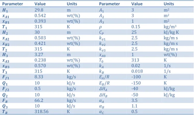
Refer to a rich plant modeling, taken from the article “Cooperative distributed model predictive control” by Stewart, Venkat, Rawlings, Wright and Pannocchia (2010); we consider in this thesis report, a plant consisting of two reactors and a separator. A stream of pure reactant A is added to each reactor and converted to the product B by a first-order reaction as illustrated in Figure 6. The product is lost by a parallel first-order reaction to side product C. The distillate of the separator is split and partially redirected to the first reactor.
The model for t 1 1 1 1 1 Figure the plant is 6: Two reactorss in series with s 1 separator and reecycle
1 1 1 1 1 1 1 1
In which for all ∈ :
exp exp
0.01 ̅ ̅ ̅ 1 Table 3: Steady state and parameters
Parameter Value Units Parameter Value Units
29.8 m 3 m2 0.542 wt % 3 m2 0.393 wt % 1 m2 315 K 0.15 kg/m3 30 m 25 kJ/kg K 0.503 wt % 2.5 kg/m s 0.421 wt % 2.5 kg/m s 315 K 2.5 kg/m s 3.27 m 1 wt % 0.238 wt % 313 K 0.570 wt % 0.02 1/s 315 K 0.018 1/s 8.33 kg/s / ‐100 K 10 kJ/s / ‐150 K 0.5 kg/s ‐40 kJ/kg 10 kJ/s ‐50 kJ/kg 66.2 kg/s 3.5 10 kJ/s 1.1 318.56 K 0.5
Chemical processes have been traditionally operated using linear controllers, although it is well recognized that a characteristic of chemical processes presenting a challenging control problem is the inherent nonlinearity of the process. Linear controllers can yield satisfactory performance, if the process is operated “close” to a nominal steady state or is fairly “linear”. Many times the process dynamic characteristics will change dramatically due to a large
disturbance or due to significant setpoint changes from an on-line optimization routine.
Consequently, chemical manufacturing processes present many challenging control problems, including nonlinear dynamic behavior. Other common process characteristics that cause control difficulty for linear and nonlinear systems alike are:
multivariable interactions between manipulated and controlled variables unmeasured state variables
unmeasured and frequent disturbances high-order and distributed processes uncertain and time-varying parameters
constraints on manipulated and state variables deadtime on inputs and measurements
3 Model Predictive Control
The only advanced control methodology which has made a significant impact on industrial control engineering is predictive control. It has so far been applied mainly in the petrochemical industry, but is currently being increasingly applied in other sectors of the process industry. The main reasons for its success in these applications are:
1. It handles multivariable control problems naturally. 2. It can take account of actuator limitations.
3. It allows operation closer to constraints (compared with conventional control), which frequently leads to more profitable operation. Remarkably short pay-back periods have been reported.
4. Control update rates are relatively low in these applications, so that there is plenty of time for the necessary on-line computations.
In addition to the “constraint-aware optimizing” variety of predictive control, there is an 'easy-to-tune, intuitive' variety, which puts less emphasis on constraints and optimization, but more emphasis on simplicity and speed of computation, and is particularly suitable for single-input, single-output (SISO) problems. This variety has been applied in high-bandwidth applications such as servomechanisms, as well as to relatively slow processes.
Model predictive control is an appropriately descriptive name for a class of model based control schemes that utilize a process model for two central tasks (i) explicit prediction of future process behavior, and (ii) computation of appropriate corrective control action required to drive the predicted output as close as possible to the desired target values. The overall objectives of an MPC may be summarized as:
• Prevent violations of input and output constraints.
• Drive some output variables to their optimal setpoints, while maintaining other outputs within specified ranges.
• Prevent excessive movement of the input variables.
• Control as many process variables as possible when a sensor or actuator is not available.
The ideas appearing to a greater or lesser degree, in all predictive controls are basically:
• dependence of the control law on predicted behavior,
• explicit use of models to predict the process output at future time instants, • calculation of control sequence minimizing an objective function, and
• receding horizon strategy, i.e., updating of input and shifting of the horizon towards the future at each time instant.
Predictive control is intuitive and used in our daily activities like walking, driving, studying and so on. Think about the course of studying in a school. Basically one has to do a set of things:
• Predict: When one sets a target for a “desired” grade, one has to plan and work towards the target. It may be too early to consider the final target at beginning of a term. Instead, one should think a few days or a few weeks ahead and predict what performance may be achieved over this shorter time window. The target within the shorter time period can be, for example, certain “desired” grades in the assignment, quiz, etc.
• Plan: Compare the predicted performance with the shorter time target. If a difference is to be expected, for example, lower than the target, then additional efforts should be considered, subject to constraints of course, such as there are only 24 hours a day.
• Act: If it is expected that the additional efforts likely make one meet the target, then the additional efforts will be put into action. Although a set of the additional efforts, for today, tomorrow, and so on, has been planned days or weeks ahead, only the effort planned for today can actually be materialized today. In the next day, the procedure of prediction and planning is repeated, and a new set of efforts is determined. Thus the next day’s action will be taken according to the new planning. This process proceeds continuously until the end of the term.
Other well-known daily-life analogies in MPC literature include crossing a road and playing chess. In chess, a good player predicts the game a few steps ahead based on the moves of the opponent, and plans a few future moves. However, only one move can actually be applied each time. Based on the following-up move of the opponent, a new set of predictions has to be made and a new set of future moves is determined as a result. This procedure is repeated throughout the game.
3.1 Historical issues on MPC in process control
When MPC was first advocated by Richalet, Rault, Testud and Papon (1976) for process control, several proposals for MPC had already been made, such as Lee and Markus (1967), and, even earlier, a proposal, by Propoi (1963), of a form of MPC, using linear programming, for linear systems with hard constraints on control. However, the early proponents of MPC for process control proceeded independently, addressing the needs and concerns of industry. Existing techniques for control design, such as linear quadratic control, were not widely used, perhaps because they were regarded as addressing inadequately the problems raised by constraints, nonlinearities and uncertainty. The applications envisaged were mainly in the petro-chemical and process industries, where economic considerations required operating points (determined by solving linear programs) situated on the boundary of the set of operating points satisfying all constraints. The dynamic controller therefore has to cope adequately with constraints that would otherwise be transgressed even with small disturbances. The plants were modeled in the early literature by step or impulse responses. These were easily understood by users and facilitated casting the optimal control and identification problems in a form suitable for existing software.
Thus, IDCOM (identification and command), the form of MPC proposed in Richalet et al. (1976,1978), employs a finite horizon pulse response (linear) model, a quadratic cost function, and input and output constraints. The model permits linear
estimation, using least squares. The algorithm for solving the open-loop optimal control problem is a “dual” of the estimation algorithm. As in dynamic matrix control (DMC; Cutler & Ramaker, 1980; Prett & Gillette, 1980), which employs a step response model but is, in other respects, similar, the treatment of control and output constraints is ad hoc. This limitation was overcome in the second-generation program, quadratic dynamic matrix control (QDMC; Garcia & Morshedi, 1986) where quadratic programming is employed to solve exactly the constrained open-loop optimal control problem that results when the system is linear, the cost quadratic, and the control and state constraints are defined by linear inequalities. QDMC also permits, if required, temporary violation of some output constraints, effectively enlarging the set of states that can be satisfactorily controlled. The third generation of MPC technology, introduced about a decade ago, distinguishes between several levels of constraints (hard, soft, ranked), provides some mechanism to recover from an infeasible solution, addresses the issues resulting from a control structure that changes in real time, and allows for a wider range of process dynamics and controller specifications (Qin & Badgwell, 1997). In particular, the Shell multivariable optimizing control (SMOC) algorithm allows for state-space models, general disturbance models and state estimation via Kalman filtering (Marquis & Broustail, 1988). The history of the three generations of MPC technology, and the subsequent evolution of commercial MPC, is well described in the last reference. The substantial impact that this technology has had on industry
is confirmed by the number of applications (probably exceeding 2000) that make it a multi-million dollar industry.
The industrial proponents of MPC did not address stability theoretically, but were obviously aware of its importance; their versions of MPC are not automatically stabilizing. However, by restricting attention to stable plants, and choosing a horizon large compared with the “settling” time of the plant, stability properties associated with an infinite horizon are achieved. Academic research, stimulated by the unparalleled success of MPC, commenced a theoretical investigation of stability. Because Lyapunov techniques were not employed initially, stability had to be addressed within the restrictive framework of linear analysis, confining attention to model predictive control of linear unconstrained systems. The original finite horizon formulation of the optimal control problem (without any modification to ensure stability) was employed. Researchers therefore studied the effect of control and cost horizons and cost parameters on stability when the system is linear, the cost is quadratic, and hard constraints are absent. A typical result establishes the existence of finite control and cost horizons such that the resultant model predictive controller is stabilizing.
3.2 Open loop optimal control problem
The system to be controlled is usually described, or approximated, by an ordinary differential equation, but since the control is normally piecewise constant, is usually modeled, in the MPC literature, by a difference equation.
Consider the system
1 , ,
where ∈ and ∈ are the state and input vector, respectively. We assume that the origin is an equilibrium point (f(0, 0) = 0).
We presumed the system to be specified in discrete time. One reason is that we are looking for solutions to engineering problems. In practice, the controller will always be implemented through a digital computer by sampling the variables of the system and transmitting the control action to the system at discrete time points. Another reason is that for the solution of the optimal control problems for discrete-time systems, we will be able to make ready use of powerful mathematical programming software. However, in many instances the discrete time model is an approximation of the continuous time model.
According to the optimal control theory, the problem is to minimize the performance index J (performance objective or cost function).
, , ,
with respect to the future control sequence of input u from the time to 1.
, 1 , … , 1
Generally the solution of the optimal control problem can be founded by solving the Hamilton-Jacobi-Bellman equation (HJB) as follow,
, min , , , 1
with the boundary condition , .
The plant model generally can be linearized around the operation point to yield the linearized plant formulation. By considering a linear system
1
where ∈ , ∈ and are calculated as
̅, , ̅,
Before introducing the quadratic cost function, it is restored to express some definitions. Expressions like and , where x, u are vectors, Q and R are symmetric matrices and indicate the transpose of vector x, are called quadratic forms, and are often written as ‖ ‖ and ‖ ‖ respectively. They are just compact representations of certain quadratic functions in several variables.
Considering a linear system and a quadratic cost function
, , 0, 0
, 0
where Q and S are state weighting or penalty and R is input weighting.
The problem is turned into Linear Quadratic Control (LQ), where the HJB approach reduced to , with .
The solution is Finite Horizon (FH) problem and completely defined by the control law
1 ′ ′ 1 ′
where ′ 1 ′ 1 1 ′ 1
Meant for continuous processes which are operating over a long time period, it would be interesting to solve the infinite horizon problem.
If we consider the Infinite Horizon (IH) cost function
, 0, 0
with the assumption of reachability of pair (A,B) and observablity of pair (A,C), where Q=C’C, then the optimal control law is With
′
such that is the unique positive definite solution of the Riccati equation, which equal to
′ ′ .
In order to consider the disturbances or unmeasurable states, Kalman predictor (KP) can be applied, where there are some equivalency of parameters in the formulation of LQ and KP. Moreover Linear Quadratic Gaussian (LQG) control can be considered where in the stochastic system, the disturbances and the initial state satisfy the assumption introduced for the KP, and the state is not measurable.
3.3 Closed‐loop _ open‐loop analysis
Through considering the system as 1 ∈ , ∈
and modifying the performance index as
, , ‖ ‖ ‖ ‖ ‖ ‖
Where 0, 0, 0 and outlining N as the so-called prediction horizon, the stated problem is formed to minimizing the above performance index J. Here we divide the general problem in three categories, and try to formulate the problem with some consideration on the stability:
1- IH-LQ:
2- FH optimal control 3- Receding Horizon (RH)
3.3.1 IH‐LQ
According to the previous result by the infinite horizon cost function and with the assumption of reachability and observability, the optimal control law is
such that is obtained by finding the P as the unique positive definite solution of the algebraic Riccati equation (ARE).
′ ′
Confined by these conditions for noted control law, the closed-loop system is asymptotically stable.
3.3.2 FH optimal control
The optimal solution is given by the state-feedback control law
, 0,1, … , 1
Where K(i) is 1 ′ 1
which is obtained by finding the P(i) as the solution of the difference Riccati equation (DRE)
1 ′ 1 1 ′ 1
with initial condition P(N)=S.
In order to find the open loop solution of FH optimal control, we recall the Lagrange equation
, 0
And define the related matrices , , , .
1 2 ⋮ 1 ⋮ 1 ⋮ 2 1 0 0 0 … … … … 0 0 … 0 0 … … … … 0 … where 0 is zero matrix.
Thus, the future state variables are given by following formula:
Moreover by defining augmented weighting matrices , with the following construction, 0 0 ⋯ 0 00 0 ⋮ ⋱ ⋮ 0 0 0 0 ⋯ 0 0 , 0 0 ⋯ 0 00 0 ⋮ ⋱ ⋮ 0 0 0 0 ⋯ 0 0
and minimizing the modified performance index ̅ with respect to U(k), the open loop solution is as follow:
, 0,1, … , 1
where depends on matrices , , and is calculated as follows.
The new modified performance index is
̅ , , ′
where with respect to the original cost function, the terms has been ignored, since it does not depend on U(k). By minimizing this new performance index which can be rewrite in the form of quadratic function of U(k), its minimum
turns out to be ′ .
Thus, by letting ′ , is obtainable.
Note1: in the nominal case, the closed-loop and the open-loop solutions coincide.
Note2: if there are constraints on the control and/or state variables, the closed-loop solution is not available, while the open-closed-loop one can be reformulated as a mathematical programming problem and can be easily solved by means of a QP (quadratic programming) method with reduced computational time.
3.3.3 In a whic law, the first over Thu beha each horiz 3 RH proble all above ca ch are defin the Reced optimizatio input uo (k) r the predic s, intuitively avior when h time step zon control m ases open-ned over a ding Horizo on problem k) of the opt ction horizo y, instead o we use a l , in effect m ). - or closed finite horiz on has bee over the p timal seque n [k+1,k+N of making th ong, but fin moving the -loop solut zon. In orde n defined i prediction h ence Uo(k). N+1] again a he horizon nite horizon horizon forw
tions are tim er to obtain n the way horizon [k,k At time k+ as shown in infinite we N, and rep ward (movi me varying n a time-inv that at any k+N] and a 1 repeat th n Figure 7. can get a s peat this op ing horizon g control la variant con y time k, so apply only he optimizat similar ptimization a or recedin aws, ntrol olve the tion at g
The RH principle allows one to obtain the state-feedback time-invariant control law.
ĸ
Intended for constrained systems, this control law is implicitly defined, while in the unconstrained case, it coincides with the first element of the open-loop solution and the first element of the closed-loop solution obtained by iterating the Riccati equation backwards from P(N)=S.
First element of the open-loop solution is:
0
First element of the closed-loop solution is:
0 , 0 1 ′ 1
Thus the receding horizon solution formed as
0 0
Noted that, it is not a-priori guaranteed that the RH control law stabilizes the closed-loop. In some cases, stability may be achieved only with the large prediction horizon.
From this point upward, the formulation of the MPC can be modified according to the applications, nevertheless the principle of receding horizon endure intrinsic in
all of these formulations. As a matter of fact that the subject of this report is setpoint tracking or in general terms, regulation problem to control some parameters within operation region in the chemical processes, the effect of introducing reference signals and disturbances with their considerations, are going to be discussed here after.
3.4 MPC formulation without integral action
Consider the system with disturbances
1
where ∈ , ∈ , ∈ , ∈ and
∈ , ∈ , ∈ .
The new cost function which is penalizing the tracking error with respect to the reference signal yo is
, ,
‖ ‖ ‖ ‖
‖ ‖
Again, we define the new matrices , , , , , with following constructions, 1 2 ⋮ 1 , 1 2 ⋮ 1 , ⋮
0 0 0 … … … … 0 0 … 0 0 … … … … 0 … , ⋮ 1 1 0 … … … … 0 0 … 0 0 … … … 00 0 … … 0
where 0 and I are zero and identity matrices.
Note here that matrices , , are time independent and they can be computed offline.
Then, the future outputs (output predictions) are formed as
By defining the future output, the problem is equivalent to minimize the modified cost function
̅ , , ° ° ′
°
which depends on the future reference signals Yo(k) and on the future
disturbances D(k). The optimal solution arise the motivation to state that, the model predictive control can “anticipate” future reference variations or the effect of known disturbances.
Note1: there is not any integral action which has been forced in the feedback control law, therefore with assumption of providing the closed-loop stability, for constant reference signal, steady state zero error regulation cannot be achieved.
Note2: In all above considered cases, the state x(k) has been assumed to be measurable. Otherwise an observer can be utilized. Likewise to estimate the disturbance d(k) when it is unmeasurable.
Note3: When the future disturbance is unknown, it is a common practice to set , 0 .
In the case of control regulation with the constant reference signals y0, by assuming that there exists a pair ̅, such that
̅ ̅
̅
, , ‖ ‖ ‖ ‖ ‖ ‖
This performance index penalizes the control deviation with respect to the desired equilibrium point.
Note 4: this performance index does not penalize the state, subsequently in this case proper observability or detectability assumption is advisable.
3.5 As t zero algo the As u inpu than algo conv and the d The the rega MPC form the aim of o error regu orithms bas inputs like F usual, the p ut u. but th n the input orithm will venient for the plant a discrete tim re are seve MPC plant arding the F mulation w setpoint tr ulation for c ed on impu Figure 8-1. plant model e before m variable th in fact pro many purp as having th me integratio eral techniq and all of Figure 8-1, with integra racking stra constant ref ulse or step Figure 8‐1: P l expresses mentioned c hemselves. oduce the poses to reg his signal as on from δu ques to inclu them involv is in which al action ategy is to ference sig p response Plugging the inte s the plant cost functio We shall s changes gard the co s input. Tha to u as bei uding this in ve augmen the integra driving the gnal, it is al models, to egral action state x in th on, penalize see in the δu, rather ontroller as at is, it is of ng included ntegration i nting the sta ators can be e system to so a comm plug an int he terms of es changes chapter 5 r than u. i producing ften conven d in the pla in a state-s ate vector. e formulate o steady st mon practice tegral action f the values s in δu, rat that the M it is theref the signal nient to reg nt dynamic pace mode The first w d as: tate e in n at s of ther MPC fore δu, gard c. el of way,
1
So the state-space form of the system plus integrators and by neglecting the disturbances is obtained:
1
1 0
0
While the Performance index with tracking error and control variation is
, ,
‖ ‖ ‖ ‖
‖ ‖
In unconstrained case, the RH control law is linear as follow
But in the block diagram view of this system, the integrator disappears due to the feedback term on signal v, as illustrated in Figure 8-2.
This aga s problem c in the enlar 1 Figure 8‐2: dis can be avoid rged system 1 appearing the in ded with an m: 1 1 → 1 1 1 1 1 ntegrator in aug n alternative 1 → 1 1 0 gmented state b e formulatio 1 block diagram on of MPC 1 → 1 and exploit 1 ting
The mat Fina whic cond Figu re is a hid rix). ally in uncon ch clearly h ditions whe ure 9. den integra nstrained c has an inte ere δx=0, s Figure al action in ase, the co gral action o that δu=0 9: Integral actio n this mode ontrol law ta on the err 0 only for t on in augmented el (indicate
akes the for
ror signal e he conditio d state block dia ed by in e rm e(k), and in on of e=0 a agram enlarged st n steady-st as illustrated tate tate d in
3.6 Extension to the basic formulation
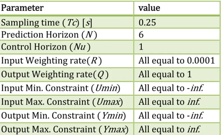
The main MPC algorithms are characterized by a number of “tricks” which make them very different from a classical LQ algorithm. Some of these tricks are Control horizon, Minimum prediction horizon, Reference filtering, Filtering of disturbances and High level optimization. Among them, we just take a short view on control horizon which will be used in the generation of MPC algorithm of chemical plants.
If the prediction horizon N is sufficiently large, the number of optimization variables (or the future control increments) can make the optimization problem difficult to solve. For this reason, and to obtain a slower control action, it is often assumed that the control variables remain constant after Nu<N time instants.
1 , , … , 1 or
0, , … , 1 In this case, the cost function can be written as follow
, ,
‖ ‖ ‖ ‖
‖ ‖
which is going to be used widely, by the advantages of easier optimization problem.
4 Stability
Early versions of MPC and generalized predictive control did not automatically ensure stability, thus requiring tuning. It is therefore not surprising that research in the 1990s devoted considerable attention to this topic. Indeed, concern for stability has been a major engine for generating different formulations of MPC. In time, differences between model predictive, generalized predictive, and receding horizon control became irrelevant; we therefore use MPC as a generic title in the consequence for that mode of control in which the current control action is determined by solving on-line an optimal control problem.
4.1 Stability analysis
Model predictive control of constrained systems is nonlinear necessitating the use of Lyapunov stability theory, that the value function (of a finite horizon optimal control problem) could be used as Lyapunov function to establish stability of receding horizon control of unconstrained systems when a terminal equality constraint is employed. These results extended that the value function as a Lyapunov function for establishing stability of model predictive control of time-varying, constrained, nonlinear, discrete-time systems (when a terminal equality constraint is employed); thereafter, the value function was almost universally employed as a natural Lyapunov function for stability analysis of model predictive control.
4.1.1 Definitions
While asymptotic convergence of the state x(k) in the form of lim → x k → 0 is a desirable property, it is generally not sufficient in practice. We would also like a system to stay in a small neighborhood of the origin when it is disturbed by a little. Formally this is expressed as Lyapunov stability.
Consider the system
1 , 0
Where is an arbitrary (discontinuous) function and ̅ is equilibrium point if ̅ ̅.
Letting ⊆ an open neighborhood of ̅ , then ̅ is stable, unstable, attractive, asymptotically stable and exponentially stable according to the following conditions:
Stable, if, for each 0, there is such that
‖ ̅‖ → ‖ ̅‖ for any 0. Unstable, if not stable.
lim → ‖ ̅‖ 0 for any ∈ . Asymptotically stable in , if it is stable and attractive in .
Exponentially stable in , if there exist 0, ∈ 0,1 such that
‖ ̅‖ ‖ ̅‖ for any 0.
The ε, δ requirement for stability definition takes a challenge-answer form. To demonstrate that the origin is stable, for any value of ε that a challenger may chose (however small), we must produce a value of δ such that a trajectory starting in a δ neighborhood of the origin will never leave the ε neighborhood of the origin.
Function : → is a K function if it is continuous, strictly increasing with 0 0.
Usually to show Lyapunov stability of the origin for a particular system, one constructs a so called Lyapunov function, i.e., a function satisfying the conditions of the following theorem.
Let ⊆ be a positively invariant set for the system
containing a neighborhood of the equilibrium x 0 .
Undertake that , , be the class K functions and assume that there exist a nonnegative scalar function : → , 0 0 such that
‖ ‖ , ∀ ∈ ‖ ‖ , ∀ ∈ ∆ ‖ ‖ , ∀ ∈
Then the origin is an asymptotically stable equilibrium in . Moreover, if ‖ ‖ ≔ ‖ ‖ , ‖ ‖ ≔ ‖ ‖ , ‖ ‖ ≔ ‖ ‖ for some , , , 0 and
, then the origin is exponentially stable in .
We use the extension of the Lyapunov theory by considering non continuous Lyapunov functions (the cost function in constrained MPC control) and refer to Figure10.
4.1.2 RH and IH‐LQ control
Considering linear system with measurable state
1
and its performance index