Computational homogenization of syntactic foams & material response subjected to extreme loads

(1)

POLITECNICO DI MILANO

Computational Homogenization of Syntactic Foams &

Material Response Subjected to Extreme Loads

School of Civil Engineering

Master of Science in Civil Engineering

Supervisor:

Prof. Stefano Mariani

Co-Advisor:

Prof. Marco Di prisco

Master of Science Thesis by:

Bahman Bahmani Ghajar

Matricola: 749454

(2)

1

Table of Figures

Figure 1- Three main classes of engineering materials, whose combination provides Composite Materials

[16] ... 10

Figure 2- Schematic representations of fibrous composites [16] ... 12

Figure 3- The spreading pattern of fibers in two different cylindrical samples ... 12

Figure 4- Schematic representation of particulate composites, a) flake composite, b) general particulate composite, c) filler composite [11] ... 13

Figure 5-Micrographs of syntactic foams [10] ... 14

Table 6 - Composite Phase Material Properties ... 15

Figure-7- Equivalent Pure Vinyl Ester RVE models ... 18

Figure 8- Equivalent Vinyl Ester RVE models with void ... 19

Table 9 - Pure Vinyl Ester RVE model results ... 20

Figure 10 - RVEs with various inclusion volume fraction ... 21

Diagram 11 – Single Inclusion RVE Young Modulus - MEMSYS ... 22

Diagram 12 - Single Inclusion RVE Young Modulus - ANALYTIC... 22

Diagram 13 – Single Inclusion RVE Poisson’s Ratio - MEMSYS ... 23

Diagram 14 – Single Inclusion RVE Poisson’s Ratio - ANALYTIC ... 23

Diagram 15 – Single Inclusion RVE Young Modulus – MEMSYS - ANALYTIC ... 24

Diagram 16 - Single Inclusion RVE Poisson’s Ratio – MEMSYS - ANALYTIC ... 24

Figure 17 – Composite Materials Tensile Modulus [9] ... 25

Table - 18 – 2D and 3D Equivalent RVE models ... 26

Table 19 – Microbaloons Properties used in Syntactic Foams ... 26

Table 20 – Microbaloons Dimensional Properties used in Syntactic Foams ... 27

Figure 21 - Asymmetric RVE models with constant length ... 28

Diagram 22 – Single Inclusion Rectangular RVE Young Modulus – Constant Length ... 29

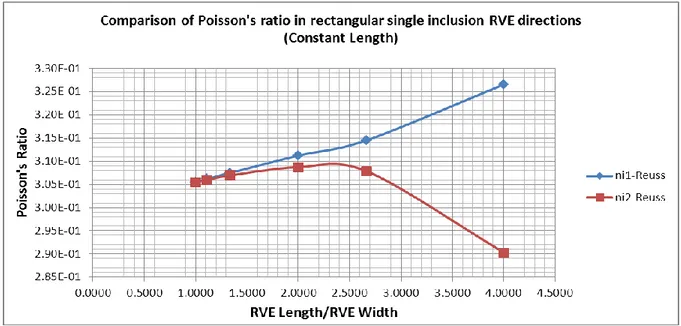
Diagram 23 - Single Inclusion Rectangular RVE Poisson’s Ratio – Constant Length ... 29

Diagram 24 - Single Inclusion Rectangular RVE Young Modulus – Constant Length... 30

Diagram 25 - Single Inclusion Rectangular RVE Poisson’s Ratio – Constant Length ... 30

Diagram 26 – Comparison of RVE Young Modulus in different directions – Voigt Bound ... 31

Diagram 27 - Comparison of RVE Poisson’s Ratio in different directions – Voigt Bound ... 31

Diagram - 28 - Comparison of RVE Young Modulus in different directions – Reuss Bound ... 32

Diagram - 29 - Comparison of RVE Poisson’s Ratio in different directions – Reuss Bound... 32

Figure 30 - Asymmetric RVEs with constant volume fraction ... 34

Diagram 31 – Single Inclusion Rectangular RVE Young Modulus – Constant Area Fraction ... 35

Diagram - 32 Single Inclusion Rectangular RVE Poisson’s Ratio – Constant Area Fraction ... 35

Diagram 33 - Single Inclusion Rectangular RVE Young Modulus – Constant Area Fraction ... 36

Diagram 34 - Single Inclusion Rectangular RVE Poisson’s Ratio – Constant Area Fraction ... 36

Diagram - 35 – Comparison of Asymmetric RVE Young Modulus – Constant Area Fraction – Voigt Bound ... 37

Diagram 36 - Comparison of Asymmetric RVE Young Modulus – Constant Area Fraction – Reuss Bound ... 37

(5)

4

Diagram 37 - Comparison of Asymmetric RVE Poisson’s Ratio – Constant Area Fraction – Voigt Bound

... 38

Diagram - 38 - Comparison of Asymmetric RVE Poisson’s Ratio – Constant Area Fraction ... 38

Figure 39 - Multi - Inclusion RVE Models ... 39

Table 40 - Multi Inclusion RVE overall properties ... 40

Table 41 - Multi Inclusion RVE overall Properties - Equivalent Models ... 40

Figure 42 - (a) Micrograph and (b) schematic representation of the microstructure of typical syntactic foam. In (b), the different phases are shown, including ‘a’ matrix, ‘b’ voids, ‘c’ particles, and ‘d’ porosity enclosed inside the particle shell [8] ... 42

Figure 43 - RVE with stochastic arrangement of inclusions in y-axis ... 43

Table 44 - Probabilistic Results of overall Properties of RVE Models with Stochastic Arrangement of Inclusions ... 44

Figure 45 - Group Codes of RVE models with Stochastic Inclusion Arrangement ... 44

Diagram 46 - RVE Young Modulus (E1) - Stochastic Results - Voigt Bound ... 45

Diagram 47 - RVE Young Modulus (E1) - Stochastic Results - Reuss Bound ... 45

Figure 48 - RVE with stochastic arrangement of inclusions - Volume Fraction 13% ... 47

Figure 50 -RVE with stochastic arrangement of inclusions - Volume Fraction 30% ... 49

Table 52 - Probabilistic results of RVE models with stochastic dispersion inclusions - Volume Fraction 0.5 ... 51

Diagram 56 – Young Modulus - Single Inclusion VS Stochastic Multi Inclusion RVE model ... 54

Diagram 57 – Poisson’s ratio - Single Inclusion VS Stochastic Multi Inclusion RVE model... 54

Diagram 58 - Young Modulus - Analytic VS Stochastic Multi Inclusion RVE model ... 55

Diagram 59 - Poisson’s Ratio - Analytic VS Stochastic Multi Inclusion RVE model ... 55

Diagram 60 – Poisson’s Ratio - Analytic VS Single Inclusion RVE model ... 56

Figure 61 – Young Modulus - Analytic VS Single Inclusion RVE model ... 56

Diagram 62 – Homogenized Young Modulus of Syntactic Foams as a Function of Inclusion Volume Fraction and Inclusion Type [28] ... 57

Diagram 63 – Average Values of Homogenization Bounds - Young Modulus – MEMSYS ... 58

Diagram 64 - Average Values Homogenization Bounds - Poisson’s Ratio Bounds – MEMSYS ... 58

Figure 65 - RVEs with different inclusion wall thickness - Volume Fraction 13% ... 62

Figure 66 - RVE with different inclusion wall thickness - Volume Fraction 3% ... 64

Figure 67 – RVE Young Modulus as a function Inclusion Membrane Thickness Ratio – Inclusion Area Fraction = 0.13 – MEMSYS results ... 65

(6)

5

Figure 68 - RVE Poisson’s Ratio as a function Inclusion Membrane Thickness Ratio – Inclusion Area

Fraction = 0.13 – MEMSYS results ... 65

Figure 69 - RVE Young Modulus as a function Inclusion Membrane Thickness Ratio – Inclusion Area Fraction = 0.13 – Analytic results ... 66

Figure 70 - RVE Poisson’s Ratio as a function Inclusion Membrane Thickness Ratio – Inclusion Area Fraction = 0.13 – MEMSYS results ... 66

Figure 71 - RVE Young Modulus as a function Inclusion Membrane Thickness Ratio – Inclusion Area Fraction = 0.13 – MEMSYS VS Analytic ... 67

Figure 72 - RVE Poisson’s ratio as a function Inclusion Membrane Thickness Ratio – Inclusion Area Fraction = 0.13 – MEMSYS VS Analytic ... 67

Figure 73 - RVE Average Young Modulus as a function Inclusion Membrane Thickness Ratio – Inclusion Area Fraction = 0.13 – MEMSYS VS Analytic ... 68

Figure 75 - RVE Young Modulus as a function Inclusion Membrane Thickness Ratio – Inclusion Area Fraction = 0.03 – MEMSYS results ... 69

Figure 76 - RVE Young Modulus as a function Inclusion Membrane Thickness Ratio – Inclusion Area Fraction = 0.03 – Analytic results ... 69

Figure 77 - RVE Poisson’s Ratio as a function Inclusion Membrane Thickness Ratio – Inclusion Area Fraction = 0.03 – Analytic results ... 70

Figure 78 - RVE Young Modulus as a function Inclusion Membrane Thickness Ratio – Inclusion Area Fraction = 0.03 – MEMSYS VS Analytic ... 70

Figure 79 - RVE Poisson’s ratio as a function Inclusion Membrane Thickness Ratio – Inclusion Area Fraction = 0.03 – MEMSYS VS Analytic ... 71

Figure 81- RVE Average Poisson’s Ratio as a function Inclusion Membrane Thickness Ratio – Inclusion Area Fraction = 0.03 – MEMSYS VS Analytic ... 72

Diagram 82 – Comparing Young Modulus and Poisson’s Ratios of RVE models with inclusion area fractions equal to 0.03 and 0.13 as a function of Inclusion Thickness Ratio - MEMSYS ... 73

Diagram 83- Comparing Young Modulus and Poisson’s Ratios of RVE models with inclusion area fractions equal to 0.03 and 0.13 as a function of Inclusion Thickness Ratio - Analytic ... 74

Diagrams 84 - Change in the Young Modulus with respect to the microballoon wall thickness [7]. ... 75

Diagram 85 - Change in the Poisson’s Ratio with respect to the microballoon wall thickness [7]. ... 75

Table - 86 – RVE models with different inclusion size distribution patterns ... 78

Figure 87 – Inclusion Pattern Type-1 ... 78

Figure 88– Inclusion Pattern Type-2 ... 79

Figure 92-Young Modulus of RVE models with different inclusion size distribution patterns ... 81

Figure 93- Poisson’s Ratio of RVE models with different inclusion size distribution patterns ... 81

(7)

6

Figure 95 – Schematic Pressure Impulse Diagram and Zones Response Behavior ... 90

Figure 96 – Pressure Impulse Diagram: P-I data inversion into pressure-time load diagram ... 92

Figure 97 - Ultimate Limit State of the Slab ... 93

Figure 98 – Simply Supported FRC slab P-I diagram (Slab thickness=100mm) [28] ... 95

Table 99 - FRC Material Properties ... 97

Diagram 100 – FRC Stress-Crack Mouth opening ... 97

Figure 101 –Constitutive Model of FRC ... 98

Figure 102 - Constitutive Model of FRC (Partial Safety Factors Applied) ... 99

Figure 103 – Characteristic Constitutive Model of FRC ... 100

Figure 104- Design Constitutive Model of FRC ... 100

Figure 105 – Pressure-Time relations of blast loads ... 103

Figure 106 - FRC slab P-I diagram selected points data ... 103

Figure 107 - Compressive Constitutive law [7] ... 113

Figure 108 - Tensile Constitutive law [7] ... 113

(8)

7

Part-1 – Computational Modeling of Syntactic Foams for Deriving the

Homogenized Properties

Abstract

Owing to the important role of Syntactic Foam composite materials in various industrial applications, having applicable information about its mechanical (constitutive) properties are of high level of efficiency for analysis and design purposes. This work aims at

deriving the bounds of the overall properties of a specific type of syntactic foam-hollow sphere glass-polymer resin- composite material. Focusing on the overall mechanical parameters of the composite material, such as; the Young modulus and the Poisson’s ratio, the investigation is centered on a computational homogenization scheme over a vast range of Representative Volume Elements (RVE) types. Several computational models of RVEs are created using a commercial code finite element analysis code, to investigate the effects of independent material manufacturing parameters, such as; inclusion particles-hollow sphere glass- membrane thickness, volume fraction and size and distribution patterns. The computational modeling procedure is arranged with a hierarchical trend, starting from simple ones, in order to assure results reliability. Furthermore, experimental results and analytic tools-MATLAB code for Voigt-Reuss bounds- are used as

(9)

8

1. Introduction and Research Outline

A great variety of Structural Engineering applications such as marine and aerospace ones strive for low density materials having high strength, modulus, and damage tolerance [1]. A class of closed-cell foams, synthesized by dispersing rigid hollow particles in a matrix material, has shown considerable promise for such applications [2][3][4]. These foams, called syntactic foams, possess considerably superior mechanical properties, making it possible to use them for load bearing structural applications. Additionally, the presence of porosity inside the hollow particles, called microballoons, leads to lower moisture

absorption and lower thermal expansion, resulting in better dimensional stability [2][3]. The size and distribution of porosity can be controlled in these foams by means of volume fraction and wall thickness of the microballoon [4][5] and other independent parameters, such as inclusions spread pattern in the matrix for one fabrication method and inclusions diameter distribution in a specific production category.

The research procedure has almost followed the same scientific trend of M.Profiri and N. Gupta [7-10]. In the research activities by M.Profiri et al. [7-10], apart from experimental studies, theoretical models that relate mechanical properties with composition of

syntactic foams are also available [7] [8]. A thorough overview of modeling efforts for particulate composites has been presented by Pal [11]. The Hashin’s technique [12] has been extended to syntactic foams by Lee and Westmann [13] to obtain a single equation for the bulk modulus and bounds for the shear modulus. Huang and Gibson estimated the elastic moduli by computing the change in strain energy due to a single hollow sphere in an infinite matrix material [14]. The differential scheme has been applied to derive expressions for Young’s modulus and Poisson’s ratio of syntactic foams containing high volume fraction of microballoons. [15] First, the elastic properties in the case of an infinitely dilute dispersion of hollow inclusions are determined. A differential scheme is then used to extrapolate the effective properties of syntactic foams for a broad range of microballoon volume fractions.

(10)

9

Having such experimental and analytic results, the current research adds computational models of every kind of composite material RVE with such characteristics. The concept of homogenization technique is explained in Chapter-3.

Other than introductory and concluding parts, the research body contains sessions on the independent input parameters which affect the RVE homogenization results, as follows:

1. Inclusion Area Fraction 2. Inclusion Volume Dispersion

3. Inclusion Membrane Thickness ratio 4. Inclusion Size Distribution pattern

Every input parameter with its domain and trend of influence is thoroughly explained through the relevant session and the results are compared with the available benchmarks. In general the target parameters are Young Modulus and Poisson’s ratio of different RVE models.

Analytic models are calculated using MATLAB code Voigt-Reuss bounds [15] with its concept explained in Appendix-A and its code text given in Appendix-B. These analytic results are benchmarks to validate computational ones of target parameters lest having solutions totally off the expected scale.

2. Composite Materials

Principles of Composite material are discussed in this chapter. In sections 2.1 an

introduction on composite materials and their features are presented. In sections 2.3.1 and 2.3.2 different types of composite materials and their constituting parts are briefly

(11)

10

2.1 Introduction

The “composite” concept is not a human invention. Wood is a natural composite material consisting of one type of polymer – cellulose fibers with good strength and stiffness- in a resinous matrix of another polymer, the polysaccharide lignin. Bone, teeth and mollusk shells are other natural composites, combining hard ceramic reinforcing phases in natural organic polymer matrices [16]. Although man was familiar with composite materials during the history, it is only in the last half century that science and technology of composite materials have developed to provide the engineering with a novel class of materials, and the necessary tools to enable us to use them properly

[16].

Figure-1 gives an idea of the most familiar composite materials. Within each group of materials- metallic, ceramic and polymeric- there are certain familiar materials which can be described as composites. Steels, ceramics and concrete all are classic examples of composite materials. These materials are well known and their mechanical properties are controlled by the form and the distribution of their micro-structures.

Figure 1- Three main classes of engineering materials, whose combination provides Composite Materials [16]

(12)

11

2.2 Properties of composite materials

These are the summary of advantages proposed by composite materials related to their mechanical properties and applications [16]:

 High resistance to fatigue and corrosion

 High strength or stiffness to weight ratio; Weight savings are significant respect to the weight of conventional metallic designs.

 Improved dent resistance.

 High resistance to impact damage

 Dimensional stability; Having low thermal conductivity and low coefficient of thermal expansion and can be tailored to comply with a broad range of thermal expansion design requirements to minimize thermal stresses.

 Less need of materials, since composite parts and structures are frequently built to shape rather than machined to the required configuration, as is common with metals.

 Excellent heat sink properties, especially carbon-carbon, combined with their lightweight have extended their use for aircraft brakes.

 Improved friction and wear properties

 Some of the disadvantages of composite materials are as follows:  High cost of raw materials and fabrication.

 Possible weak transverse properties, since usually composites expected to provide a high strength along a special direction like the direction of fibers.

 Reuse and disposal may be difficult.

 Difficult structural and health monitoring inspections

New technologies have provided a variety of reinforcing fibers and matrices that can be combined to form composites having a wide range of properties.

Since the composites are capable of providing structural efficiency at lower weight, as compared to equivalent metallic structures, they have emerged as the primary materials for future use such as marine and aerospace applications [17, 18].

2.3 Composite material classification

Composite materials can be classified according to the type of reinforcement used. Two broad classes of composites are the fibrous and the particulate ones.

Each one also can be subdivided into specific categories, as discussed below [20].

(13)

12

2.3.1. Fibrous composites

A fibrous composite consists of either continuous or chopped fibers, suspended in a matrix material. Schematics of both types of fibrous composites are shown in Figure-2

Figure 2- Schematic representations of fibrous composites [16]

Continuous fibers are characterized as having a very high length to diameter ratio. They are generally stronger and stiffer than bulk materials [19].

Composites, in which the reinforcements are discontinuous fibers, can be produced to have either random or biased orientation. The discontinuities can produce a material response that is anisotropic. Moreover, continuous fibers may be either single or multilayered ones. The single layer continuous fiber composites can be either unidirectional or woven and multilayered composites are generally referred to as laminates.

A very good example of fibrous composite materials could be Fiber Reinforced Concrete (FRC). In fact the fiber itself could be from a vast category of materials ranging from synthetic plastics to steel, etc. However the most common type is SFRC which stands for Steel Fiber Reinforced Concrete. This material has proven to have several advantages compared to traditional Reinforced Concrete and concrete paste. The addition of fibers to the concrete which is a particulate composite itself – due to presence of aggregates in the cement paste – gives an additional tensile stiffness and strength to the material in a rather homogeneous pattern with respect to its spread over the casting volume.

(14)

13

2.3.2 Particulate composites

A particulate composite is characterized as being composed of particles suspected in a matrix. Particles can have virtually any shape, size or configuration. An example of well-known particulate composites is concrete. A schematic of several types of particulate composites is shown in Figure -4. There are two categories of particulates: flake and filled/skeletal.

A flake composite is generally composed of flakes with large ratio of platform area to thickness, suspended in a matrix material. A filled/skeletal composite is composed of a continuous skeletal matrix filled by a second material. The response of a particulate composite can be either anisotropic or orthotropic.

Figure 4- Schematic representation of particulate composites, a) flake composite, b) general particulate composite, c) filler composite [11]

(15)

14

In fact Syntactic foams which are the subject of the current research are categorized as particulate composites which are synthesized by dispersing hollow microspheres, called microballoons, in a matrix material [21]. In the coming chapter the effects of several microbaloon properties on the overall properties of a particulate composite material – syntactic foam- is investigated by computational method.

(16)

15

3. Homogenization

3.1. Introduction

A composite is a heterogeneous material whose properties vary from point to point on a length scale ‘l’, called microscale, which is much smaller than both the scale of variation of the loading conditions and the overall body dimensions which are characterized by the length ‘L’ defining the macroscale. At the macroscale level the composite can be

regarded as a continuum medium characterized by uniform properties; such properties will be in the following equivalently referred to as effective, or homogenized, or overall, or macroscopic [23]. Any region occupied by material over which the composite

properties are constant at the microscale level will be called phase; therefore, a composite material is a continuum in which a number of discrete homogeneous continua are bonded together. Any region of the heterogeneous body characterized by a length scale ‘L’ such that l/L≪ 1, which is then macroscopically seen as homogeneous, is called

Representative Volume Element hereafter shortened in RVE [23].

One fundamental step in both the design and the analysis of syntactic foams concerns the evaluation of their linear elastic behavior. The computation of the so-called effective (i.e., macroscopic) elastic moduli of syntactic foams can be tackled by means of homogenization techniques [23].

In the current research, in order to estimate the overall properties of syntactic foams made of glass sphere (as inclusion) and vinyl ester (as matrix), computational models of various geometrical properties are created to represent each material RVE with its corresponding characteristics. On the other hand there are analytic methods which are introduced in the following.

In the following, the material properties of the Sphere-Glass and Matrix Vinyl Ester are assumed as Figure - 6:

Composite Phase Young Modulus (GPa) Poisson’s Ratio

Vinyl Ester 3.21 0.3

Sphere Glass 60 0.21

(17)

16

3.1.1 Analytic Procedure

There is a wide range of analytic methods which are in fact mathematical models with various assumptions based on the composite materials structure and properties. Eshelby solution [23][24], Dilute approximation[23][24], Voigt and Reuss bounds[25] and Hashin–Shtrikman bounds [26][27] as four methods in order to derive the overall properties of composite material RVE for a linear elastic constitutive behavior assumption [23]. While M.Profiri [7] takes a combination of the methods of Lee and Westmann [13] besides Dilute approximation [23][24] and Hashin’s technique as introduced by Torquato [12].

In this thesis a simple technique based on Voigt and Reuss Bounds is presented in order to set benchmarks as a comparing tool for the computational results, besides the

experimental results.

Voigt and Reuss approaches respectively assume the state of strain or stress to be uniform inside the RVE [22]. They are known to provide bilateral bounding for the elastic moduli of multiphase systems, even though bounds are not tight. Analytical results furnished by the two approaches are here used to validate the numerical results. The mathematical procedure is explained in Appendix-A and the MATLAB code is given in Appendix –B.

3.1.2 Computational Procedure

The computational procedure of the homogenization is a combination of finite element analysis and a numerical procedure which uses the outcomes. RVE is assumed a square shape with its phases of different materials. The RVE boundary condition is described under plane stress conditions. No assumption of an isotropic behavior is valid a prior to the homogenization. Considering the plane stress condition, the RVE is subjected to unit stresses on its boundary and afterwards strains over the area of RVE finite elements are derived and averaged. Having three different elements in a 2D stress vector, three equations are created which results in Young Modulus and the Poisson’s ratio in two directions. Applying the strains on boundary conditions and calculating the stress values over the RVE gives another set of results for Young Modulus and the Poisson’s ratio. The two sets of results provide the bounds by which the RVE overall constitutive properties are constrained.

(18)

17

3.2 Independent Parameters

The computational tool used for modeling the explained problem is a non-commercial code called MEMSYS. The following parameters effects have been investigated on the composite material overall mechanical parameters:

1. Inclusion Area Fraction: The Volume Fraction of Inclusion Particles that constitute the composite material. This means the volume ratio of present

inclusions with respect to the material overall volume. In this case as the analysis is done using 2D models, Inclusion Area Fraction is considered as the

independent parameter. Inclusion area corresponds to the inclusion circle area including the void and not merely to the solid part.

2. Inclusion Dispersion Model: This parameter explains the morphology of the

inclusions dispersion in matrix material with respect to each other. Considering a 2D plane, there might be one equal dispersion of the inclusions in the material resulting in equal distances between inclusion particles in longitudinal and

transverse directions or a kind of dispersion that results in larger distances between inclusion particles in longitudinal direction compared with transverse one or vice-the-versa.

3. Inclusion Membrane Thickness Ratio: Hollow spheres are used as inclusions in

the currently investigated material; the membrane thickness of these hollow spheres is a key parameter to the deriving Syntactic Foam overall mechanical properties. Considering the substitution of circles with spheres due to the 2D nature of the modeling tool.

4. Inclusion Size Distribution Pattern: In a real manufacturing procedure,

controlling a bulk mass of inclusion material (glass sphere), it can be seen that glass spheres don’t have a precise and unique size; rather there’s a distribution of sizes in the bulk mass of a product category with a defining nominal average and variance for the sphere diameter. Considering a discrete distribution to convert the problem for a computational modeling procedure, a series of inclusion distribution types are compared with each other to control the effect of the inclusion particles diameter size distribution on the overall mechanical properties of the

(19)

18

In the following ‘E’ stands for Young Modulus and ‘ni’ for Poisson’s Ratio. The indices “1” and “2” beside ‘E’ and ‘ni’ show the corresponding parameter in the horizontal and vertical directions of the RVE plane respectively.

3.2.1.1. Modeling tool (MEMSYS) validation; Homogenous RVE

In this section the capacity of MEMSYS code and the created models are checked for single material models by comparing physically equal models with mathematically and computationally different inputs.

The whole trial procedure is divided into four parts as follows:

1. Primarily a square RVE model (L=200 μm) is created, the material properties of Vinyl ester is assigned to the single part model.

2. The previous model is created with a single inclusion whose mechanical properties are the same of the matrix. (R=18 μm)

Figure-7- Equivalent Pure Vinyl Ester RVE models

*Models which are created in the third and fourth steps must have the same overall properties.

(20)

19

3. The model of the second step is created with a single difference of omitting the partitioned circle to create a hole instead of the circular part. (R=18 μm)

4. The model of third step is created with the only difference of partitioning a circular annulus around the circular hole. (Rext=20 μm)

Figure 8- Equivalent Vinyl Ester RVE models with void

*Models which are created in the third and fourth steps must have the same overall properties.

(21)

20

Results are as follows:

Table 9 - Pure Vinyl Ester RVE model results

As it’s evident in the Table-9 the corresponding values of Young Modulus and Poisson’s Ratio are very close to one another. Results model codes 1 and 2, which are representing a square volume element of the Vinyl Ester, could be considered as totally equal in two procedures. Comparing the results of the model codes 3 and 4, again the values match up to the forth decimal digit.

RVE size 200 μ.m

Model Model code E1(GPa) ni1 E2(GPa) ni2

Simple Rectangle 1 3.21 0.3 3.21 0.3

Rectangle with filled-in inclusion 2 3.21 0.3 3.21 0.299999999

Rectangle with hole inside (R hole = 18μ.m) 3 3.209422 0.3000079 3.209422 0.3000079

Rectangle with hollow inclusion (R int = 18μ.m) 4 3.209423 0.3000079 3.209423 0.3000079

Model

Simple Rectangle 1 3.21 0.3 3.21 0.3

Rectangle with filled-in inclusion 2 3.21 0.3 3.21 0.3

Rectangle with hole inside (R hole = 18μ.m) 3 2.984525 0.30087 2.984525 0.30087

Rectangle with hollow inclusion (R int = 18μ.m) 4 2.98451 0.3008729 2.98451 0.3008729

Reuss

(22)

21

3.2.1.2. Single Inclusion RVE Modeling with different Inclusion Area

Fractions

In this step, the real case RVE models are created using one single inclusion. The

inclusion area fraction of the composite material is modeled by assigning various values to the dimension length of the square shape RVE.

(23)

22

*As stated before an analytic method is used as a reference for the computational results. The following charts compare the Young modulus and Poisson’s ratio of RVE models with different inclusion volume fractions.

Diagram 11 – Single Inclusion RVE Young Modulus - MEMSYS

(24)

23

Diagram 13 – Single Inclusion RVE Poisson’s Ratio - MEMSYS

(25)

24

The average value of the MEMSYS bounds is calculated and shown in the diagram using the “avg” index.

Diagram 15 – Single Inclusion RVE Young Modulus – MEMSYS - ANALYTIC

Diagram 16 - Single Inclusion RVE Poisson’s Ratio – MEMSYS - ANALYTIC Referring to the results diagrams; for area fractions between 0 to 0.3, as a result of inclusions area fraction increase; all the charts show an increasing trend in the Young Modulus expect the MEMSYS Voigt bound which has a decreasing trend with a low inclination with respect to the other trends. While the average computational results

(26)

25

which are shown as E-avg shows an increasing trend again. For area Fraction equal to 0.5 the results show unpredictable divergences. This could be explained by the fact that in these models the ratio between phase material dimension and the RVE length is large so that the limits of an acceptable RVE is breached, this is well explained by Nemat-Nasser [22], where a ratio between is defined as, the maximum phase material entity size over the RVE length, this ratio shall be bound by a maximum value in order to have a meaningful volume which can represent the accepted concept of a RVE. This is the reason why Multi-Inclusion RVE models better function in homogenization procedure to result the overall values of RVEs with such inclusion fraction ratios.

Figure-17 shows the results of an investigation [9] where the inclusion volume fraction of the material has been changed and the tensile modulus of the material is investigated through a series of experiments. In the computational homogenization procedure by MEMSYS the applied unit stress and strains are positive, therefore the parameter to be compared with its results is the tensile modulus, while compressive modulus changing trend with respect to volume fraction variation is shown in the referred article [9].

Figure 17 – Composite Materials Tensile Modulus [9]

The results in figure-17 are for area fractions which this thesis does not include a specific range of them. In fact the current research is based on 2D RVE models with a circular inclusion which could also be considered as 3D RVE models with a cylindrical inclusion. For a 2D computational model geometry of a particulate single-inclusion composite material RVE, there is a physical allowance of maximum inclusion diameter equal or less

(27)

26

than the RVE size, which leads to a maximum area or volume fraction of 78%. While in the numerical results [9] volume fraction refers to ratio which consists of the volume of spherical inclusions divided to the overall volume (3D RVE with spherical inclusion). In order to find the equivalent geometries between 2D and 3D RVEs, considering equal volumes of inclusion material between a 3D RVE with a spherical inclusion and a 3D RVE with a cylindrical inclusion, Table-18 is created. The external radius of the 3D RVE with spherical inclusion is the dependent parameter which is derived as a result of RVE parameters:

Table - 18 – 2D and 3D Equivalent RVE models

The Alphanumeric codes VE220, VE320, VE370, VE460 stands for different composite materials with respect to the inclusion type density. This parameter is in fact a function of the hollow inclusion membrane thickness which varies from 5 μm to 25 μm in practic.

Table 19 – Microbaloons Properties used in Syntactic Foams L Rext Volume Fraction L Rext Volume Fraction

50.00 24.65 0.50 50.00 20.00 0.50 65.00 26.91 0.30 65.00 20.00 0.30 75.00 28.22 0.22 75.00 20.00 0.22 100.00 31.06 0.13 100.00 20.00 0.13 150.00 35.56 0.06 150.00 20.00 0.06 200.00 39.13 0.03 200.00 20.00 0.03 400.00 49.31 0.01 400.00 20.00 0.01

RVE 3D - Spherical Inclusion RVE 2D - Cylindric Inclusion Equivalent RVE Models

(28)

27

Including the theoretically used inclusion type which is used in the current chapter, with a VE710 code, the following table is created:

Table 20 – Microbaloons Dimensional Properties used in Syntactic Foams

Considering the volume (area) fraction range from 0.3 to 0.5; the experimental results [9] in the figure-17 and the MEMSYS results shown in Figure - 12 could be compared. All the results vary within an acceptable meaningful range, while there’s an absolute

mismatch between their variation trend; the trend in the experimental results of the Figure-14 show a decreasing inclination while the average MEMSYS bounds results show an increase. This could be due to the fact that the MEMSYS models for area fractions over 30% shall not be reliable as explained before based on Nemat Nasser [22] indications about the ratio between phase size with respect to RVE size and also because of the assumed constitutive model in the homogenization procedure which does not consider fractal and plastic behaviors. It is noteworthy that for volume fractions over 40%, the probability of direct contact between inclusions are relatively high and this might also change the modeling basic assumptions completely considers a complete interaction between inclusions and matrix. In the coming chapter where the stochastic dispersion of inclusions through Multi-Inclusion RVE models is described, a corrected version of the diagrams investigating the effect of the inclusion area fraction is rendered. This correction is specifically applied for the range between 30% and 50% inclusion area fraction.

3.2.1.3. Asymmetric Rectangular RVE Modeling

In this step rectangular RVE models are created instead of former square models, in case of an uneven dispersion of the inclusions in the matrix in a regular way, such

arrangements of RVE models could be resulted in the real case manufactured material.

On the other hand, by comparing the overall parameters (Young modulus and Poisson’s ratio) of these models with the corresponding square ones the validity of the models and the computational tool (MEMSYS) could be certified.

Rext (μm) Thickness(μm) Real Density (kg/cm3) Nominal Density (kg/cm3)

35 0.521 219.978 220

40 0.878 322.076 320

40 1.052 384.216 370

40 1.289 467.966 460

(29)

28

Two different categories of models are created for this case: 1. Rectangular RVE models with constant length

2. Rectangular RVE models with constact inclusion area fraction

3.2.1.3.1-Constant Length RVE Models

In these models, the RVE width is changing in every model and the effect of uneven dispersion of the inclusion particles in main perpendicular axes are investigated, regardless of the composite material inclusion particles area fraction.

(30)

29

The results are as follows:

Diagram 22 – Single Inclusion Rectangular RVE Young Modulus – Constant Length

(31)

30

Diagram 24 - Single Inclusion Rectangular RVE Young Modulus – Constant Length

(32)

31

Diagram 26 – Comparison of RVE Young Modulus in different directions – Voigt Bound

(33)

32

Diagram - 28 - Comparison of RVE Young Modulus in different directions – Reuss Bound

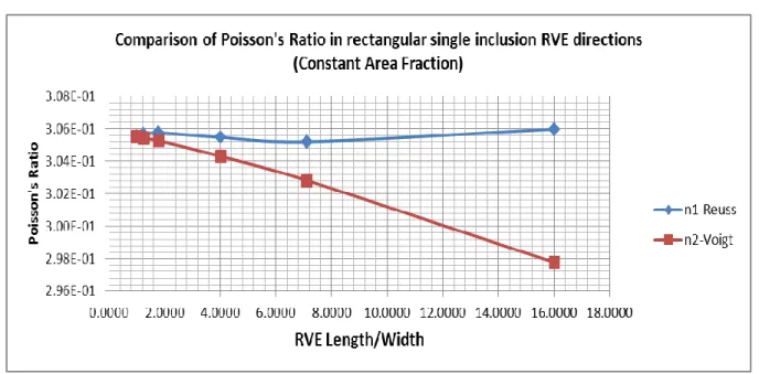
Diagram - 29 - Comparison of RVE Poisson’s Ratio in different directions – Reuss Bound

The increase of the ratio of RVE length to its width means the decrease of inclusion area fraction which its results are already obtained, while the constant length of the RVE model gives the opportunity to investigate the effects of an uneven dispersion of the inclusions.

(34)

33

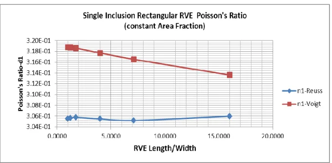
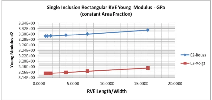
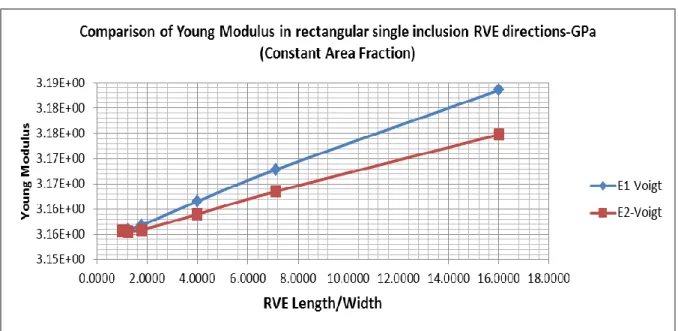
3.2.1.3.2. Constant Area Fraction RVE models

In these models the effect of uneven dispersion of the inclusion particles are investigated, considering a unique inclusion particle area fraction for every model, in other words the area fraction of models are set to be unchanged and the rectangular model width and length are changed to maintain the RVE area.

(35)

34

Figure 30 - Asymmetric RVEs with constant volume fraction

Diagrams 31 to 38 compare the Young modulus and Poisson’s ratio of various models of the same main direction which are shown using d-1 and d-2 on the chart vertical axis; d-1 refers to the longitudinal axis and d-2 to the transverse one.

(36)

35

Diagram 31 – Single Inclusion Rectangular RVE Young Modulus – Constant Area Fraction

(37)

36

Diagram 33 - Single Inclusion Rectangular RVE Young Modulus – Constant Area Fraction

(38)

37

Diagram - 35 – Comparison of Asymmetric RVE Young Modulus – Constant Area Fraction – Voigt Bound

Diagram 36 - Comparison of Asymmetric RVE Young Modulus – Constant Area Fraction – Reuss Bound

(39)

38

Diagram 37 - Comparison of Asymmetric RVE Poisson’s Ratio – Constant Area Fraction – Voigt Bound

Diagram - 38 - Comparison of Asymmetric RVE Poisson’s Ratio – Constant Area Fraction

The results show that, for a constant volume (area) fraction of inclusions, having larger ratios of RVE length to width or in practice larger distances between inclusions in their spreading model, the Young Modulus of the material is increased in both directions and the Poisson’s Ratio is decreased in both directions. However the difference is quite negligible.

(40)

39

3.2.1.4. Multi-Inclusion RVE modeling

In this step RVE models are created with two or more inclusions. The RVE shape is squared and the inclusions spacing with respect to each other is precisely equal. Two models are created, using two and four inclusions in a horizontal row.

Figure 39 - Multi - Inclusion RVE Models

The results are given and used in the next step to validate the code results in case of multi material models.

3.2.1.5. Modeling tool (MEMSYS) validation; Multi-inclusion RVE -

Asymmetric RVE

In the Tables 40 and 41 two groups of RVE models – each consisting of two RVE models – overall mechanical properties are shown. Each color shows one RVE group and every row of the Table 40 and 41 corresponds to the properties of one composite material. It can be seen that the area fraction of RVE models of the same group are equal. Based on the fundamental analytic definition of the overall mechanical properties of an RVE

(41)

40

model, the validity of MEMSYS results and the code functionality is verified up to a precise extent, in the next paragraph.

Table 40 - Multi Inclusion RVE overall properties

Considering the geometries of RVE models, the overall properties of the Multi-inclusion RVE in direction-2 (Vertical axis of RVE) should be equal to the overall properties of the asymmetric Single-inclusion RVE in direction-1 (Horizontal axis of RVE). The

corresponding values are given below:

Table 41 - Multi Inclusion RVE overall Properties - Equivalent Models Length Width/Length Number of inclusions E1 E2 ni1 ni2

200 1 4 3.0500E+00 3.0828E+00 3.5991E-01 3.5605E-01

200 0.25 1 3.0954E+00 3.0613E+00 3.5431E-01 3.5828E-01

200 1 2 3.1063E+00 3.1104E+00 3.3599E-01 3.3555E-01

200 0.5 1 3.1112E+00 3.1068E+00 3.3542E-01 3.3591E-01

MEMSYS Voigt RVE

Length Width/Length Number of inclusions E1 E2 ni1 ni2

200 1 4 3.5380E+00 3.5548E+00 3.3034E-01 3.1883E-01

200 0.25 1 3.5722E+00 3.6709E+00 3.2653E-01 2.9035E-01

200 1 2 3.3789E+00 3.3775E+00 3.1077E-01 3.1134E-01

200 0.5 1 3.3803E+00 3.3856E+00 3.1122E-01 3.0875E-01

RVE MEMSYS Reuss

200 1 4 3.0500E+00 3.0828E+00 3.5991E-01 3.5605E-01

200 0.25 1 3.0954E+00 3.0613E+00 3.5431E-01 3.5828E-01

200 1 2 3.1063E+00 3.1104E+00 3.3599E-01 3.3555E-01

200 0.5 1 3.1112E+00 3.1068E+00 3.3542E-01 3.3591E-01

MEMSYS Voigt RVE

200 1 4 3.5380E+00 3.5548E+00 3.3034E-01 3.1883E-01

200 0.25 1 3.5722E+00 3.6709E+00 3.2653E-01 2.9035E-01

200 1 2 3.3789E+00 3.3775E+00 3.1077E-01 3.1134E-01

200 0.5 1 3.3803E+00 3.3856E+00 3.1122E-01 3.0875E-01

(42)

41

In each table the results shown in the same color must match, as it is evident the Voigt results match perfectly while there are some minor differences for some of the Reuss bound results. This mismatch could be explained based on the error due to small ratio between the RVE length (width) and phase material element size as explained before. In the RVE model with its length equal to 200 μm and its width equal to 50 μm, this ratio is large and this results in results without desired precision. The remedy to avoid such results from these types of models is using Multi-Inclusion RVE models, in fact RVE length is increased and the geometry of such RVE models includes inclusions with their rather smaller sizes with respect to the RVE length. Thus the target ratio between the phase material size and the RVE length is reduced. To elaborate the concept more thoroughly, referring to the explanations regarding the computational procedure of homogenization [23] a composite material is a continuum in which a number of discrete homogeneous continua are bonded together. Considering length scale ‘l’ as microscale and any region of the heterogeneous body characterized by a length scale ‘L’ such that l/L≪ 1, which is then macroscopically seen as homogeneous [23]. The RVE length in investigated models in figure-39 stand for the length ‘L’ and the phase material size correspond to ‘l’. The smaller is l/L ratio, the homogeneity of the macroscopic scale is more preserved and thus the homogenization results are expected to be more precise.

3.2.2. Models Inclusion Dispersion

Syntactic foams are fabricated by dispersing hollow microspheres in a matrix material with a twofold purpose: to embed closed cell porosity in the matrix, thus reducing the material density while controlling the size and distribution of the porosity; and to

reinforce the matrix phase by using particles of a material stiffer than the matrix [8]. The “dispersion” of the inclusions in the matrix for manufacturing purposes gives a stochastic nature to the inclusions arrangement at its RVE scale level.

In this section such a stochastic dispersion is modeled in the computational approach using multi-Inclusion RVEs.

Figure-42 shows the stated randomness. The micrographs [9] show the presence of entrapped air or voids which are not considered in the current computational models by MEMSYS.

(43)

42

Figure 42 - (a) Micrograph and (b) schematic representation of the microstructure of typical syntactic foam. In (b), the different phases are shown, including ‘a’ matrix, ‘b’ voids, ‘c’ particles, and ‘d’ porosity enclosed inside the particle shell [8]

3.2.2.1 Multi-Inclusion RVE modeling with stochastic arrangement of

inclusions

In this section, in order to represent a more realistic model of the composite material the arrangement of inclusion particle is assumed to be randomly chosen.

Considering the 4 inclusion model which was discussed the previous chapter, the coordination of each inclusion particle is randomly assigned by computational code. In the first step, the vertical coordinate is a random number and the horizontal one of the inclusion particle is as same as the 4 inclusion model shown in figure-38.

(44)

43

Figure 43 - RVE with stochastic arrangement of inclusions in y-axis

For sake of having an acceptable random field, 100 stochastic models are created and the results are categorized in 4 groups of 25 models, in order to compare the probabilistic values of each group instead of 100 models results and facilitate making conclusions. The overall properties of each model are derived using MEMSYS. Applying the probabilistic

(45)

44

calculations over the overall mechanical results of each group of 25 models, the average and standard deviation of every group is calculated, comparing the results of four groups in the Table-44 and Diagrams 46 and 47; it can be deduced the random dispersion of inclusions in the matrix doesn’t affect its overall mechanical properties significantly.

Table 44 - Probabilistic Results of overall Properties of RVE Models with Stochastic Arrangement of Inclusions

*All the models have the same area fraction and inclusion properties, the changing parameters are the inclusions coordination in vertical direction.

The models are categorized in groups with numeric codes as shown the Table –

Figure 45 - Group Codes of RVE models with Stochastic Inclusion Arrangement Voigt

N Average STdv Average STdv Average STdv Average STdv

1--25 3.01199 0.009325 3.027173 0.012336 0.368851 0.002031 0.36699 0.002402 26--50 3.007553 0.008359 3.020688 0.010297 0.369882 0.001766 0.368263 0.002012 51--75 3.011085 0.012123 3.023448 0.016823 0.369173 0.002731 0.367659 0.003293 75--100 3.012803 0.009662 3.025059 0.013604 0.368825 0.002122 0.367323 0.002608 Total 3.010858 0.010017 3.024092 0.013481 0.369183 0.0022 0.367558 0.002623 E1 E2 ni12 ni21 Reuss

1--25 3.586401 0.011111 3.58069 0.007866 0.317655 0.002906 0.317967 0.001723 26--50 3.591666 0.009259 3.582789 0.006296 0.31617 0.002526 0.318095 0.001193 51--75 3.589919 0.015406 3.582681 0.010056 0.316713 0.004021 0.317933 0.001667 75--100 3.589019 0.010077 3.58118 0.006891 0.316722 0.002766 0.31825 0.001884 Total 3.589251 0.011684 3.581835 0.007841 0.316815 0.003107 0.318061 0.001617 ni21 E1 E2 ni12 Group N 1 1--25 2 26--50 3 51--75 4 75--100

(46)

45

The following diagrams show the overall Young Modulus of the RVE in the horizontal direction (d1).

Diagram 46 - RVE Young Modulus (E1) - Stochastic Results - Voigt Bound

(47)

46

In the next step both vertical and horizontal coordinates are randomly assigned. This latter case is an RVE model which can represent the real case manufactured material micro-scale so precisely, from the point of view that is related to the inclusions dispersion in the composite matrix.

In this step, the former procedure is done for 4 groups of 100 models. Having a more number of models increases the level of certainty in the probabilistic model. Every group represents an RVE model with a different area fraction.

The area fractions 0.13, 0.22, 0.3 and 0.5 are chosen to represent wide range of the composite material diluteness. As it is evident in the Figure-48 the inclusions are present in the RVE with a low volume fraction with respect to the matrix with a large remaining area to accept more inclusions, while Figure-51 shows that there’s no space to add any more inclusions due to the dense population of the inclusions in the RVE.

(48)

47 Inclusion Area Fraction=0.13

(49)

(50)

(51)

Figure 51 - RVE with stochastic arrangement of inclusions - Volume Fraction 50% In fact there are 100 models for every “Area Fraction” of inclusions in the composite material. The models are categorized into 4 groups of 25. After deriving the results of the

(52)

51

overall mechanical parameters, the average and standard deviation values of each group of 25 models are calculated and compared to check the influence of the inclusions

random. Then the average value of 100 models overall mechanical parameters is assumed as the representative value for that area fraction from a stochastic computational

modeling procedure.

The probabilistic results of each volume fraction group of 100 models are shown below:

Area fraction = 0.5

Table 52 - Probabilistic results of RVE models with stochastic dispersion inclusions - Volume Fraction 0.5

Area fraction = 0.3

Reuss

1--25 5.414 0.036 5.417 0.034 0.403 0.010 0.402 0.010 26--50 5.436 0.030 5.420 0.041 0.399 0.008 0.404 0.010 51--75 5.425 0.032 5.419 0.036 0.401 0.008 0.403 0.009 75--100 5.426 0.045 5.440 0.032 0.403 0.011 0.399 0.009 Total 5.425 0.036 5.424 0.037 0.401 0.009 0.402 0.009 E1 E2 ni12 ni21 Voigt

1--25 2.6906E+00 6.2896E-03 2.6903E+00 6.4225E-03 5.0314E-01 1.1452E-03 5.0318E-01 1.1718E-03

26--50 2.6867E+00 6.9657E-03 2.6868E+00 6.9923E-03 5.0384E-01 1.2851E-03 5.0384E-01 1.2898E-03

51--75 2.6881E+00 7.4923E-03 2.6881E+00 7.1950E-03 5.0359E-01 1.3763E-03 5.0358E-01 1.3177E-03

75--100 2.6866E+00 5.6166E-03 2.6867E+00 5.6729E-03 5.0386E-01 1.0256E-03 5.0384E-01 1.0367E-03

Total 2.6880E+00 6.7211E-03 2.6880E+00 6.6611E-03 5.0361E-01 1.2323E-03 5.0361E-01 1.2206E-03

E1 E2 ni12 ni21

Reuss

1--25 4.3270E+00 9.3371E-02 4.3325E+00 9.3846E-02 3.3747E-01 1.5925E-02 3.3605E-01 1.5370E-02

26--50 4.3212E+00 8.0289E-02 4.3101E+00 8.3189E-02 3.3689E-01 1.3510E-02 3.4107E-01 1.4608E-02

51--75 4.3123E+00 8.4799E-02 4.3195E+00 8.8168E-02 3.3974E-01 1.4764E-02 3.3776E-01 1.5448E-02

75--100 4.3011E+00 8.4590E-02 4.3081E+00 7.6982E-02 3.4212E-01 1.5257E-02 3.3946E-01 1.2847E-02

Total 4.3154E+00 8.5150E-02 4.3175E+00 8.5015E-02 3.3906E-01 1.4809E-02 3.3859E-01 1.4506E-02

E1 E2 ni12 ni21

Voigt

1--25 2.7740E+00 4.4497E-02 2.7694E+00 4.8365E-02 4.5124E-01 8.8158E-03 4.5201E-01 9.4883E-03

26--50 2.7801E+00 4.1275E-02 2.7810E+00 3.9331E-02 4.4996E-01 8.1271E-03 4.4980E-01 7.7951E-03

51--75 2.7843E+00 4.1866E-02 2.7800E+00 4.3827E-02 4.4923E-01 8.2854E-03 4.4994E-01 8.6251E-03

75--100 2.7862E+00 4.3298E-02 2.7844E+00 4.1979E-02 4.4880E-01 8.5690E-03 4.4909E-01 8.3080E-03

Total 2.7811E+00 4.2364E-02 2.7787E+00 4.3204E-02 4.4981E-01 8.3763E-03 4.5021E-01 8.5158E-03

(53)

52

Area fraction = 0.22

Area fraction = 0.13

Reuss

1--25 3.9672E+00 4.1592E-02 3.9697E+00 4.3776E-02 3.3003E-01 8.3869E-03 3.2878E-01 8.6955E-03

26--50 3.9497E+00 3.5104E-02 3.9556E+00 3.4968E-02 3.3361E-01 7.0861E-03 3.3082E-01 7.3536E-03

51--75 3.9640E+00 4.4332E-02 3.9600E+00 3.8245E-02 3.2970E-01 9.2282E-03 3.3105E-01 7.3099E-03

75--100 3.9748E+00 3.2038E-02 3.9799E+00 3.3822E-02 3.2886E-01 6.8534E-03 3.2691E-01 7.2695E-03

Total 3.9639E+00 3.9077E-02 3.9663E+00 3.8490E-02 3.3055E-01 8.0371E-03 3.2939E-01 7.7498E-03

E1 E2 ni12 ni21

Voigt

1--25 2.8652E+00 3.3295E-02 2.8670E+00 3.6073E-02 4.1902E-01 6.7745E-03 4.1877E-01 7.1921E-03

26--50 2.8733E+00 2.9678E-02 2.8759E+00 2.8174E-02 4.1734E-01 5.9189E-03 4.1695E-01 5.6785E-03

51--75 2.8747E+00 3.4656E-02 2.8750E+00 3.4927E-02 4.1714E-01 6.9732E-03 4.1710E-01 7.0045E-03

75--100 2.8579E+00 2.7680E-02 2.8561E+00 2.7534E-02 4.2061E-01 5.5591E-03 4.2088E-01 5.5459E-03

Total 2.8678E+00 3.1707E-02 2.8685E+00 3.2430E-02 4.1853E-01 6.3942E-03 4.1842E-01 6.4995E-03

E1 E2 ni12 ni21

Reuss

1--25 3.5832E+00 1.2283E-02 3.5807E+00 9.1042E-03 3.1817E-01 3.6213E-03 3.1943E-01 2.2867E-03

26--50 3.5819E+00 1.3829E-02 3.5830E+00 1.2014E-02 3.1902E-01 3.6167E-03 3.1842E-01 2.9559E-03

51--75 3.5825E+00 1.1291E-02 3.5780E+00 1.3907E-02 3.1810E-01 2.5261E-03 3.2028E-01 3.5907E-03

75--100 3.5775E+00 1.0946E-02 3.5782E+00 1.2075E-02 3.1965E-01 3.1043E-03 3.1955E-01 3.5637E-03

Total 3.5813E+00 1.2161E-02 3.5800E+00 1.1897E-02 3.1873E-01 3.2631E-03 3.1942E-01 3.1673E-03

E1 E2 ni12 ni21

Voigt

1--25 3.0088E+00 1.2578E-02 3.0065E+00 1.4325E-02 3.7018E-01 2.6182E-03 3.7047E-01 2.8522E-03

26--50 3.0073E+00 1.7168E-02 3.0073E+00 1.8781E-02 3.7038E-01 3.5431E-03 3.7038E-01 3.7474E-03

51--75 3.0096E+00 2.0549E-02 3.0084E+00 1.7526E-02 3.6997E-01 4.1079E-03 3.7010E-01 3.7186E-03

75--100 3.0139E+00 1.3036E-02 3.0121E+00 1.3488E-02 3.6909E-01 2.6876E-03 3.6931E-01 2.7463E-03

Total 3.0099E+00 1.6109E-02 3.0086E+00 1.6077E-02 3.6991E-01 3.2853E-03 3.7007E-01 3.2813E-03

(54)

53

Checking the average values of four groups in the Tables 52, 53, 54 and 55 it is evident that the composite material (RVE) Young Modulus and Poisson’s Ratio don’t change considerably as a result of the inclusions arrangement change over the RVE. This leads to the Statistical Homogeneity of composite introduced overall properties (Young Modulus and Poisson’s Ratio) with respect to the inclusions arrangement.

*If any possible RVE of a composite material has the same properties then the composite material is Statistically Homogeneous. [23]

(55)

54

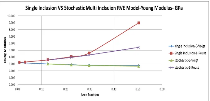
The diagrams 56 and 57 compare the results which were obtained from single inclusion models and the stochastic models of the same area fraction.

Diagram 56 – Young Modulus - Single Inclusion VS Stochastic Multi Inclusion RVE model

(56)

55

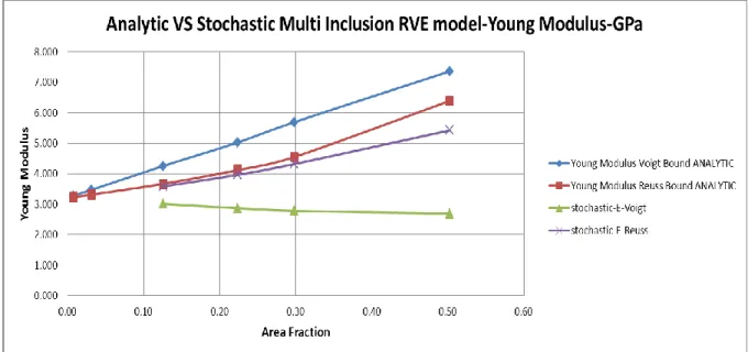
Diagrams 58 and 59 compare the results which were obtained from analytic estimation of overall properties and the stochastic models of the same area fraction.

Diagram 58 - Young Modulus - Analytic VS Stochastic Multi Inclusion RVE model

(57)

56

Diagrams 60 and 61 compare the results which were obtained from single inclusion models and the analytic bounds.

Diagram 60 – Poisson’s Ratio - Analytic VS Single Inclusion RVE model

(58)

57

Diagram-62 [28] which shows Homogenized analytic and numerical values of Young Modulus of syntactic composite made of different inclusion types which are introduced in Figure-19 is used as a benchmark to compare the MEMSYS homogenization results. The comments and concluding remarks are given at the end of this section.

Diagram 62 – Homogenized Young Modulus of Syntactic Foams as a Function of Inclusion Volume Fraction and Inclusion Type [28]

(59)

58

Diagrams 63 and 64 compare the average results which were obtained from single inclusion models and the average results of the stochastic models of the same area fraction.

Diagram 63 – Average Values of Homogenization Bounds - Young Modulus – MEMSYS

Diagram 64 - Average Values Homogenization Bounds - Poisson’s Ratio Bounds – MEMSYS

(60)

59

Reviewing the Diagrams 56 and 57, the significant change with respect to the Single-Inclusion model results which were given in chapter 3.2.1 is the correction of the Reuss bound results by using multi-inclusion results. In multi-inclusion RVE models results, the visible deviation of results due to area fraction transgress over 30% is not visible anymore and the results follow the expected path. This is in fact a result of resolving the problem of largeness of the ratio between the phase material size over the RVE length (width). Using Multi-Inclusion RVE, the RVE length becomes larger with respect to the phase material specific size (i.e. inclusion membrane thickness) and the ratio falls within an acceptable range. This issue is well-explained in 3.2.1.5.

Diagram-64 shows the average of Young Modulus Voigt and Reuss bounds for multi-inclusion RVEs. The multi-inclusion used in these models has a nominal density of 710 kg/cm3 as stated in Table-20. Diagram-62 shows the numerical results of homogenization of syntactic foams made of standard inclusions – Table-19. Comparing the inclusion used in the MEMSYS models with the ones used in models with their Young Moduli stated in Diagram-62, the most similar inclusion to the one used in MEMSYS models with nominal density of 710 kg/cm3 is K37.

Comparing the MEMSYS results in Diagram 64, with numerical results of the syntactic foam made of inclusion code K37 in Diagram 62, the increasing trend of the Young Modulus as a result of inclusion volume fraction increase, is evident in both models. The values of Young Modulus resulted from MEMSYS models, with inclusions having a nominal density of 710 kg/cm3 are around 10% more than those of K37 numerical results. This could be explained based on the thicker membrane –Table-20- of MEMSYS models inclusions with respect to K37 which makes the composite stiffer. The effect of

(61)

60

3.2.3. Inclusion membrane thickness ratio

Overall mechanical properties of Syntactic Foams also depend on the hollow particulate inclusion membrane thickness. In industrial forms the common values of the inclusion thickness ranges between 5 μm to 25 μm [8]. While in theory there could be inclusions even without any inner void part. Thus, the effect of inclusion membrane thickness on the overall properties of syntactic foam RVEs is investigated in the following [7].

3.2.3.1. Single Inclusion RVE Modeling with different Inclusion Thickness

Ratio Inclusion

As it was explained, other than inclusion volume (area) fraction, the other key parameter in the overall parameters of a composite material is the wall (membrane) thickness of the inclusions [7]. This issue is investigated by creating single inclusion models for

inclusions with different wall thickness. A series of inclusions with different wall thicknesses are adopted for two RVE sizes which result in two composite models with inclusion area fractions equal to 0.13 and 0.03. The inclusion area fraction equal to 0.13 is adopted as a common value and the area fraction equal to 0.03 is a rather comparable model to the infinitely dilute RVE model explained by Mariani et al. [7]. The concept of infinitely dilute RVE model in theory is a single particle in an infinite matrix medium [7]. The infinite matrix medium in this thesis is approximately substituted with a RVE size 200 μm and a common inclusion with a diameter equal to 40 μm, which corresponds to the composite material model with area fraction equal to 0.03.

Inclusion thickness ratio is the independent parameter which stands for:

In the article by Porfiri et al. [7] the wall thickness ratio is considered the same while the diagrams are set as a function of the independent parameter (1-η).

Therefore, the evolution of η from 0 towards 1, means a transition from a non-hollow fully filled inclusion towards a void of 40 μm diameter. Referring to Table-19 and 20, it is noteworthy to highlight that the diameter of a common particulate inclusion is 40 μm.

(62)

61

Analytic results are calculated using the MATLAB code which is given in the Appendix - B, the diagrams of the stated results are rendered in order to be used as a benchmark for the computational results.

(63)

62

(64)

(65)

64

(66)

65

The results are shown in the Diagrams 67 to 83.

RVE model-1: RVE length = 100 Volume fraction = 0.13

Figure 67 – RVE Young Modulus as a function Inclusion Membrane Thickness Ratio – Inclusion Area Fraction = 0.13 – MEMSYS results

Figure 68 - RVE Poisson’s Ratio as a function Inclusion Membrane Thickness Ratio – Inclusion Area Fraction = 0.13 – MEMSYS results

(67)

66

Figure 69 - RVE Young Modulus as a function Inclusion Membrane Thickness Ratio – Inclusion Area Fraction = 0.13 – Analytic results

Figure 70 - RVE Poisson’s Ratio as a function Inclusion Membrane Thickness Ratio – Inclusion Area Fraction = 0.13 – MEMSYS results

(68)

67

Figure 71 - RVE Young Modulus as a function Inclusion Membrane Thickness Ratio – Inclusion Area Fraction = 0.13 – MEMSYS VS Analytic

Figure 72 - RVE Poisson’s ratio as a function Inclusion Membrane Thickness Ratio – Inclusion Area Fraction = 0.13 – MEMSYS VS Analytic

(69)

68

Figure 73 - RVE Average Young Modulus as a function Inclusion Membrane Thickness Ratio – Inclusion Area Fraction = 0.13 – MEMSYS VS Analytic

Figure 74 - RVE Average Young Modulus as a function Inclusion Membrane Thickness Ratio – Inclusion Area Fraction = 0.13 – MEMSYS VS Analytic

Computational homogenization of syntactic foams & material response subjected to extreme loads

POLITECNICO DI MILANO