A beam finite element model including warping. Application to the dynamic and static analysis of bridge decks

A BEAM FINITE ELEMENT MODEL INCLUDING WARPING

Application to the dynamic and static analysis of bridge decks

Diego Lisi

Tesi di laurea in Ingegneria Civile

Relatore:

Prof. Pier Giorgio Malerba

iii

RIASSUNTO

Questa tesi si propone come obiettivo lo studio degli effetti dinamici e statici in travi continue con sezioni a parete sottile attraverso lo sviluppo di un modello a elementi finiti.

Quando una sezione in parete sottile soggetta a torsione è aperta la sua deformabilità è considerevolmente maggiore di quella di sezioni compatte e chiuse, per effetto della maggiore deformazione sezionale dovuta a questo tipo di sollecitazione, che ne determina un maggiore ingobbimento.

L’analisi esatta di travi a parete sottile considerando il fenomeno di ingobbimento è di complessa implementazione numerica, a causa dell’ elevata esigenza computazionale delle soluzioni matematiche.

Le teorie classiche di travi sono analizzate inizialmente di modo che possa essere ottenuta una formulazione di equazioni governative in termini di spostamenti generalizzati. Si sono utilizzati i principi variazionali per determinare un modello approssimato e per caratterizzare un elemento finito di trave per l’analisi di sezioni in parete sottile.

In ambito statico, travi continue con asse rettilineo sono analizzate, mentre in dinamica le vibrazioni flesso-torsionali di questi elementi sono investigate sia in regime libero sia forzato da un carico mobile concentrato. I risultati di queste analisi sono comparati con le soluzioni teoriche ottenute per elementi di trave.

L’obiettivo di questo elaborato è di proporre un modello generalizzato di trave per profili in parete sottile, utile per il progetto di ponti ferroviari realizzati nelle reti ad alta velocità. Un caso di studio di ponte a varie campate è illustrato per valutare il comportamento dinamica di differenti sezioni.

PAROLE CHIAVE: sezioni a parete sottile, impalcato da ponte, metodo degli elementi finiti, ingobbamento, elemento di trave, analisi dinamica, carichi mobili.

v

ABSTRACT

The present dissertation deals with the study of the dynamic and static effects on continuous beams of thin-walled cross-sections through the formulation of a finite element.

When a thin-walled cross-section of a beam structure has open profile the deformability greatly exceeds that of a compact section, because of to the out-of-plane deformations of this type of shapes when acted by torsion, being this effect due to the warping of the cross-section.

The exact analysis of thin walled beams considering the warping phenomena is usually difficult in its implementation by numerical codes for their mathematical solutions that are too complicated for routine calculations.

The classic beam theories are analyzed to obtain the set of equations governing the problem. The variational principles are used in order to obtain an approximation model and purpose a finite beam element for the analysis of thin-walled beams.

In static, straight and generally supported structures are analyzed, while in dynamic the torsional and lateral free-vibration and forced vibration is investigated. The results of the analysis and the compliance with the classic beam theory are discussed.

The aim of the work is to propose a generalized thin-walled beam model for the railway high-velocity bridge analysis and design. A simple numerical example of multi-span bridge is illustrated in order to evaluate the performance of different types of cross-sections when dynamic effects are considered.

KEYWORDS: thin-walled beams, bridge deck, finite element method, warping, beam element, dynamic analysis, moving load.

vii

ACKNOWLEDGEMENTS

I would like to express my gratitude for all who contributed in a way or another in the accomplishment of this work.

Most importantly, I would like to thank my supervisors Pr. Francisco Virtuoso and Pr. Ricardo Vieira. Their helpful comments, advices, suggestions and contributions regarding all the critical aspects of my thesis have been very profitable over the last year.

I would thank all the colleagues of the Civil Engineering (DECivil) department for being extremely helpful and for creating a comfortable working environment. Their friendship has provided a real support.

Many thanks for my family: they made it possible for me to come to Lisbon.

Ringrazio in modo particolare la disponibilità e gentilezza del Prof. Pier Giorgio Malerba del Dipartimento di Ingegneria Strutturale, relatore al Politecnico di Milano del seguente elaborato.

ix

INDEX

1.2. Objectives of the work ... 17

1.3. Layout of the work... 18

1.4. Original contributions of the present work ... 19

2. LITERATURE REVIEW AND BACKGROUND INFORMATION ... 21

2.1. Historical evolution of thin walled beam theories ... 21

2.2. Methods of analysis for thin walled beam structures ... 22

2.3. Lateral-torsional forced vibrations of thin walled beam structures ... 23

3. THIN-WALLED BEAMS EQUATIONS ... 25

3.1. Cross-section analysis ... 25

3.1.1. Kinematics and strains ... 25

3.1.2. Potential energy formulation ... 32

3.1.3. Elastic center and shear center ... 35

3.1.3. The direct method for the warping properties evaluation ... 37

3.1.4. A generalized method for the section properties evaluation ... 39

3.1.5. Kinetic energy formulation ... 53

3.2. Static analysis ... 54

3.2.1. Equilibrium and stresses ... 55

3.2.3. Basic load cases ... 60

3.3. Dynamic analysis ... 69

3.3.1. Equations of motion ... 69

3.3.2. Analysis of torsional free vibrations on thin-walled beams ... 73

4. FINITE ELEMENT APROXIMATION ... 77

4.1. Beam displacements discretization ... 78

4.1.1. Continuity ... 78

4.1.2. Approximation functions ... 79

4.2. The static formulation of the finite element ... 81

x

4.2.2. The thin-walled beam element considering an additional DOF of warping ... 85

4.2.3. Selected load cases ... 93

4.3. The dynamic formulation of the finite element ... 110

4.3.1. The formulation of a weak form for the uncoupled torsion ... 110

4.3.2. The element mass matrix considering an additional DOF of warping ... 112

4.3.3. The undamped free-vibration ... 119

4.3.4. Examples ... 122

5. ANALYSIS OF DYNAMIC RESPONSE TO MOVING LOADS ... 133

5.1. The procedure of mode superposition ... 133

5.1.1. Uncoupled equations of motion with damping ... 134

5.1.2. Modal response to loading ... 135

5.2.Numerical modeling of dynamical response ... 136

5.2.1.Element property matrices... 136

5.2.2.Time-stepping Newmark’s method ... 138

5.3. Numerical example... 139

5.3.1.Actions on the bridge and structural properties ... 139

5.3.2.Undamped free-vibration analysis ... 141

5.3.3.Forced-vibrations analysis and mode-superposition procedure ... 143

6. CONCLUSIONS AND FINITE DEVELOPMENTS ... 155

6.1. General remarks ... 155

6.1. Conclusions ... 155

6.2. Future developments ... 156

7. References ... 159

xi

INDEX OF FIGURES

Figure 3.1 - Principal displacements and system coordinates of the beam. ... 26

Figure 3.2 - Rotation of a I-Section around a general point P. ... 26

Figure 3.3- Axial displacements of an I-Beam due to axial effect and bending for planes (x,y) and (x,z). ... 27

Figure 3.4 - Vanishing of the shear strain of mid-surface (left) and distribution along the wall thickness for open cross-sections (right). ... 27

Figure 3.5 - Rotation of open cross-section. ... 28

Figure 3.6 – Geometric interpretation of the sectorial coordinate. ... 29

Figure 3.7 – Geometric interpretation of h(s) and hs(s). ... 31

Figure 3.8 – Open cross-section with N elements. ... 37

Figure 3.9 – Global reference axis and local axis of the element. ... 40

Figure 3.10 - Example of two-celled cross-section. ... 42

Figure 3.11 – Sketch of the three-branches open section. ... 45

Figure 3.12 - Warping function distribution. ... 46

Figure 3.13 – Sketch of the double-T bridge deck section. ... 47

Figure 3.14 – Warping function distribution. ... 48

Figure 3.15 – Box section of a bridge deck [m]. ... 49

Figure 3.16 - Warping function distribution. ... 50

Figure 3.17 – Two-cells section of a bridge deck [m]. ... 51

Figure 3.18 - Warping function distribution. ... 53

Figure 3.19 – Generalized displacements of a C cross-section beam. ... 59

Figure 3.20 – Forces in a C cross-section beam. ... 59

Figure 3.21 – S-S beam (L=2m) acted upon uniform torque. ... 62

Figure 3.22 - 𝜑 value of a S-S beam acted by uniform torque (analytical solution). ... 63

Figure 3.23 – 𝜑′ value of a S-S beam acted by uniform torque (analytical solution). ... 63

Figure 3.24 - 𝑀𝜔 of a S-S beam acted by uniform torque (analytical solution). ... 63

Figure 3.25 – Distribution of the torsion 𝑇𝑆 and 𝑇 of a S-S beam acted by uniform torque (analytical solution). ... 64

Figure 3.26 – S-S beam (L=2m) acted upon concentrated torque at midspan. ... 64

Figure 3.27 – 𝜑 value of a S-S beam acted by concentrated torque (analytical solution). ... 65

Figure 3.28 – 𝜑′ value of a S-S beam acted by concentrated torque (analytical solution). ... 65

Figure 3.29 – 𝑀𝜔 of a S-S beam acted by concentrated torque (analytical solution). ... 65

Figure 3.30 - Distribution of the torsion 𝑇𝑆 and 𝑇 of a S-S beam acted by concentrated torque (anal. solution). ... 65

Figure 3.31 – Three continuous span beam acted by uniform torque at midspan. ... 66

Figure 3.32 – 𝜑 value of a continuous three spans beam acted by uniform torque (analytical solution). ... 67

Figure 3.33 – 𝜑′ value of a continuous three spans beam acted by uniform torque (analytical solution). ... 67

Figure 3.34– 𝑀𝜔of a continuous three spans beam acted by uniform torque (analytical solution). ... 67

Figure 3.35 - Distribution of the torsion 𝑇𝑆 and 𝑇 of a continuous three spans beam acted by uniform torque (analytical solution). ... 68

xii

Figure 3.36 – Distribution of the torsion 𝑇𝜔 and 𝑇 of a continuous three spans beam acted by uniform

torque (analytical solution). ... 68

Figure 3.37 – Coupling between torsion and bending displacements for a C-beam. ... 73

Figure 3.38 – Simply supported beam analyzed by (Gere, 1954). ... 74

Figure 3.39 – Values of the ratio r for the first 8 torsional vibration modes. ... 75

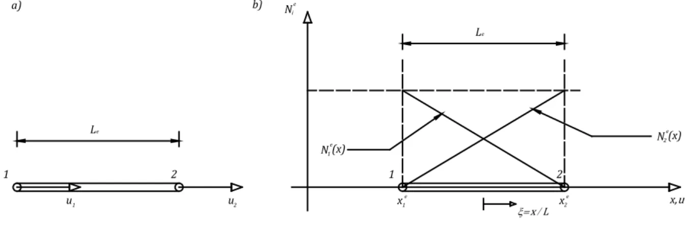
Figure 4.1 – Degrees of freedom and shape functions of the two node elements. ... 79

Figure 4.2 - Two-node Euler-Bernoulli element. ... 80

Figure 4.3 –Thin walled beam element subject to uncoupled torsion. ... 84

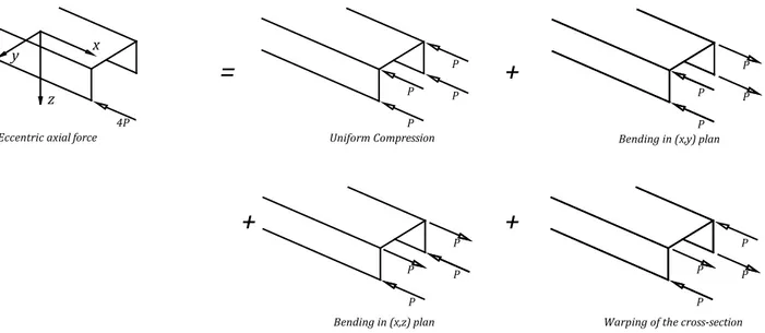
Figure 4.4 – Effects of the application of a general axial force on a thin walled beam (Cedolin, 1996). ... 87

Figure 4.5 – Thin-walled C-beam element displacement referred to two axis. ... 91

Figure 4.6 –Thin-walled C-beam element displacements described by the elastic center axis. ... 93

Figure 4.7 – Non-dimensional coordinate system. ... 94

Figure 4.8 – 𝜑 value of a S-S beam acted by uniform torque (FEM solution). ... 95

Figure 4.9 – 𝜑′ value of a S-S beam acted by uniform torque (FEM solution). ... 95

Figure 4.10 - 𝑀𝜔 of a S-S beam acted by uniform torque (FEM solution). ... 95

Figure 4.11 – Torsion 𝑇 of a S-S beam acted by uniform torque (FEM solution). ... 95

Figure 4.12 – 𝜑 value of a S-S beam acted by concentrated torque (FEM solution). ... 96

Figure 4.13 – 𝜑′ value of a S-S beam acted by concentrated torque (FEM solution). ... 96

Figure 4.14- 𝑀𝜔 of a S-S beam acted by concentrated torque (FEM solution). ... 96

Figure 4.15 - Torsion 𝑇 of a S-S beam acted by concentrated torque (FEM solution). ... 97

Figure 4.16 – Coordinate system of the three continuous spans beam. ... 97

Figure 4.17 - 𝜑 value of a T-C-S beam acted by uniform torque (FEM solution). ... 98

Figure 4.18 - 𝜑′ value of a T-C-S beam acted by uniform torque (FEM solution). ... 98

Figure 4.19 - 𝑀𝜔 of a T-C-S beam acted by uniform torque (FEM solution). ... 98

Figure 4.20 – Tosion 𝑇 of a T-C-S beam acted by uniform torque (FEM solution). ... 99

Figure 4.21 – Convergence of the 𝑀𝜔 value as function of the mesh refinement. ... 100

Figure 4.22 – ABAQUS element B310S and integration points for I-beam section. ... 100

Figure 4.23 - Longitudinal model of a bridge numerical example. ... 102

Figure 4.24 – Box-section of the bridge deck. ... 102

Figure 4.25 – Double-T section of the bridge deck. ... 102

Figure 4.26 – Lane model for general types of vertical loads. ... 103

Figure 4.27 – Loading in the cross-section plane. ... 105

Figure 4.28 –Loading in the longitudinal direction. ... 105

Figure 4.29 – Coupling effect between torsion and transversal displacement. ... 105

Figure 4.30 – Displacements and rotation of the bridge model with double-T section (FEM model). ... 106

Figure 4.31 – Shear force 𝑉𝑧 and bending moment 𝑀𝑧 along the elastic center axis. ... 107

Figure 4.32 – Torsion moment 𝑀𝑡 and warping moment 𝑀𝜔 along the elastic center axis. ... 107

Figure 4.33 - Twist values along the beam axis for the double-T section and for the Box section. ... 108

Figure 4.34 – Saint Venant torsion contribution for the double-T section and for the Box section. ... 108

xiii

Figure 4.36 –Thin-walled C-beam element and uncoupled kinematic field. ... 116

Figure 4.37 - Thin-walled C-beam element and coupled kinematic field. ... 119

Figure 4.38 - Ratio r for 8 vibration modes in a S-S beam. Solution obtained by the presented model. ... 124

Figure 4.39 - Ratio r for 8 vibration modes in a C-S beam. Solution obtained by the presented model. ... 124

Figure 4.40 - Ratio r for 8 vibration modes in a C-C beam. Solution obtained by the presented model. ... 124

Figure 4.41 - Influence of boundary conditions on the 1st _{mode frequency. ... 125}

Figure 4.42 - Influence of boundary conditions on the 2nd mode frequency. ... 126

Figure 4.43- Influence of boundary conditions on the 3rd mode frequency. ... 126

Figure 4.44 - Influence of boundary conditions on the 4th mode frequency. ... 126

Figure 5.1 – Example of supported beam element acted by a constant and eccentric moving load. ... 135

Figure 5.2 – Experimental values of the damping coefficient for different bridge spans. (Cunha, 2007). ... 137

Figure 5.3 – Applied loads on a supported beam along 𝑥-direction. ... 137

Figure 5.4 – Linear interpolation for the time intensity at time t... 138

Figure 5.5 – Bridge layout of the cross-section and sketch of the actions considered. ... 140

Figure 5.6 – Damping coefficients variation for the double-T bridge section. ... 144

Figure 5.7 – Damping coefficients variation for the box girder bridge section. ... 144

Figure 5.8 – Layout of the simply supported beam and moving load... 145

Figure 5.9 – Mid-span dimensionless displacement comparison (𝛼 = 0.5). ... 146

Figure 5.10 – Mid-span dimensionless displacement comparison (𝛼 = 1). ... 146

Figure 5.11 – Mid-span dimensionless displacement comparison (𝛼 = 2). ... 146

Figure 5.12 - Mid-span dimensionless displacement comparison (𝛼 = 0.5, 𝛽 = 0.1). ... 147

Figure 5.13 - Mid-span dimensionless displacement comparison (𝛼 = 1, 𝛽 = 0.1). ... 147

Figure 5.14 - Mid-span dimensionless displacement comparison (𝛼 = 2, 𝛽 = 0.1). ... 147

Figure 5.15 – Longitudinal beam-like model (a) and layout of the cross-section analyzed (b). ... 148

Figure 5.16 – Dynamic influence lines of the displacement uz at the section AA’ (double-T section). ... 149

Figure 5.17 - Dynamic influence lines of the twist φ at the section AA’ (double-T section). ... 149

Figure 5.18 - Dynamic influence lines of the displacement uy at the section AA’ (double-T section). ... 150

Figure 5.19 - Dynamic influence lines of the displacement uz at the section AA’(box girder section).. ... 150

Figure 5.20 - Dynamic influence lines of the twist φ at the section AA’ (box girder section). ... 151

Figure 5.21 - Dynamic influence lines of the displacement uy at the section AA’ (box girder section). ... 151

Figure 5.22 – Displacement 𝑢𝑧 for the two bridge sections analyzed (load speed: 420 km/h). ... 151

Figure 5.23 – Horizontal displacements of the bridge cross-section(load speed: 420 km/h). ... 152

Figure 5.24 - Twist of the bridge sections (load speed: 420 km/h). ... 152

Figure 5.25 – Maximum vertical deflection of the section AA’ for various speed values. ... 153

Figure 5.26 – Maximum twist rotation of the section AA’ for various speed values. ... 153

Figure 5.27 – Displacement of the point P of the double-T section. ... 154

Figure 5.28 – Dynamic influence line of the displacement 𝑢𝑧𝑃. ... 154

Figure A.0.1 – Cross-section layouts ... 161

Figure A.0.2 – Sectorial coordinate for the open and closed cross-sections. ... 162

xv

INDEX OF TABLES

Table 2.1 – Analogy between the theories of Vlasov and Bernoulli. ... 21

Table 3.1 - Cross-Section parameters. ... 33

Table 3.2 – Beam loads per unit length. ... 34

Table 3.3 - Section data input of the code assembled. ... 45

Table 3.4 – Section data output of the code assembled. ... 46

Table 3.5 - Section data input of the code assembled. ... 47

Table 3.6 – Section data output of the code assembled. ... 48

Table 3.7 - Section data input of the code assembled. ... 49

Table 3.8 – Section data output of the code assembled. ... 50

Table 3.9 - Section data input of the code assembled. ... 51

Table 3.10 – Section data output of the code assembled. ... 52

Table 3.11 – Equilibrium equations and boundary conditions. ... 58

Table 3.12 - Cross-section layouts and position of the elastic and shear center. ... 61

Table 3.13 – Boundary conditions for the three continuous spans beam. ... 66

Table 3.14 – Dimensionless warping moment at supports. ... 68

Table 3.15 – Characteristics of the beam element analyzed by (Gere, 1954). ... 74

Table 4.1 – Smoothness of functions (Fish & Belytschko, 2007). ... 78

Table 4.2 – Displacement field and approximation functions. ... 85

Table 4.3 – Beam element displacements and corresponding axis of reference ... 90

Table 4.4 – Cross-section layout characteristics. ... 94

Table 4.5 – Boundary conditions of the beam. ... 94

Table 4.6 – FEM discretization for the continuous three spans beam. ... 97

Table 4.7 – Boundary conditions of the three continuous spans beam. ... 97

Table 4.8 – Decrease of the relative error of 𝑀𝜔/𝑚𝐿2 for different finite element meshes. ... 99

Table 4.9 – Characteristics of the beam Elements loaded. ... 101

Table 4.10 – Comparison of results between current model and ABAQUS element. ... 101

Table 4.11 – Flexural characteristics of the bridge deck cross-sections. ... 103

Table 4.12 – Section properties of the bridge cross-sections. ... 104

Table 4.13 – Cross-section properties and torsion parameters. ... 104

Table 4.14 – Boundary displacement fixed at nodes. ... 106

Table 4.15 – Boundary conditions of the bar (S-S,C-S,C-C). ... 123

Table 4.16 – Characteristics of the steel beam cross-section layout and bar length. ... 127

Table 4.17 – Torsional vibration modes for a simply supported I-beam. ... 128

Table 4.18 - Characteristics of the cross-section layout and span lengths. ... 129

Table 4.19 - Torsional vibration modes for a three continuous spans I-beam. ... 129

Table 4.20 – Characteristics of the cross-sections and structural systems compared. ... 130

Table 4.21 – Mode vibration frequencies for the S-S beam and relative errors compared with ABAQUS. ... 130

xvi

Table 5.1 – General actions of the railway bridge. ... 140

Table 5.2 – Undamped vibration modes and respective modal frequencies for the double-T bridge section. ... 141

Table 5.3 – Vibration modes for the double-T bridge section (frequencies in [Hz]). ... 142

Table 5.4 – Undamped vibration modes and respective modal frequencies for the box bridge section. ... 143

Table 5.5 – Rayleigh coefficients for the bridge cross-sections considered. ... 144

Table 5.6 – Properties of the simply supported beam-like bridge discretization. ... 145

Table 5.7 – Set of train velocities considered. ... 148

Table 5.8 – Parameters considered for the numerical simulation of the current analysis. ... 149

Table 5.9 – Maximum displacement values for some characteristic velocities... 153

17

1. INTRODUCTION

1.1. General introduction

Throughout history, thin walled structures become common construction elements. The reason for their extensive use is probably due to the trend of reducing the structural weight and to minimize building materials. This very natural optimization strategy constituted an important design principle for the realization of any type of structure.

For the large use of thin walled sections their behavior have been widely studied from many authors and the simplest way to consider these elements, when involved in frame structures analysis, is the adoption of longitudinal beam elements. This is possible whenever the response of slender elements is investigated, such as the analysis of steel structures, buildings, bridges or other complex structures.

The thin walled cross-sections appear in different forms, from simple hot rolled steel beams to the complex hull of a ship or the bridge deck shape. In all these cases the knowledge of flexural, axial and torsional response is essential for the analysis of the internal forces and the stress field acting on the sections.

The present analysis considers railway bridges with a cross-section that can be considered thin-walled. For these structures, the torsion has a very important role to investigate their structural response. It is well known that the torsional response of a thin-walled open section is very different from that of a compact or closed shaft. When the section of a bridge has an open profile the out-of-plane longitudinal deformations greatly exceed those of a closed section, either in a multicellular or in a monocellular type. This happens because of the physical behavior of this kind of shapes in their response to torsion solicitations: for this reason, in the field of bridges and advanced constructions, torsion is an important aspect to be considered in the design and the warping of the open sections cannot be neglected.

Warping introduces longitudinal strains as the section twists and significantly affects the torsional stiffness. In the case of thin-walled beams with open cross-section, the constraint of the axial warping strains provides the primary source of torsional stiffness.

1.2. Objectives of the work

The dynamic study of railway bridges has been greatly enhanced during the recent years: the means of transport are faster and heavier, while the structure over which they move are more slender and generally constituted by thin-walled cross sections.

This study presents a generalized beam model based on the FEM1 _{technology for the static and dynamic} analysis of thin-walled beams. According to the Euler-Bernoulli theory, six degrees of freedom for each end of the finite element are considered. A 7th _{degree of freedom will be considered in the finite element developed in order} to describe the warping displacements.

1 _{Finite element method}

18

The consideration of the cross section warping is based on the Vlasov beam theory for thin walled open sections and extended to the closed thin-walled section by introducing a modified warping parameter according to the Benscoter theory.

In statics, straight and generally supported structures are analyzed, while in dynamics the torsional and lateral free and forced vibration analysis is presented. In the last part of the work an example of moving force acting eccentrically is presented, in order to evaluate the performance of this type of elements in bridge design.

The focus of the work is the analysis of double-T bridge open sections and box girder sections. An uncoupled flexural motion in the vertical plane and a coupled lateral-torsional vibration are studied showing the effect of the sectional properties on the mode frequencies. When forced vibration are considered, this work obtains dynamic influence lines for the twist rotation, the horizontal and vertical displacement of the midspan point for different train velocities, load magnitudes and eccentricity. The purpose is the formulation of a simple tool that enables the basic analysis of multi-span bridges through adequate beam models that consider the thin-walled open or closed section effects.

1.3. Layout of the work

In chapter 1 a general introduction to the current work is presented. The motivations and developments needed are illustrated considering the contribution of the thin walled beam elements to the civil engineering applications.

The chapter 2 proposes a general review of the thin-walled beam theories with particular attention to the torsion problem considering the different cross-section behaviors. A general survey summarizes also the application in dynamic analysis of these studies and the results obtained with the theoretical approach.

The chapter 3 presents the theory of thin-walled beams in statics and dynamics. Starting from the description of the beam element kinematics, the governing differential equations for thin-walled cross-sections are deduced by using the energetic approach. Several load cases are presented in static analysis considering the exact results, while in dynamics a torsional vibration analysis is presented.

The chapter 4 deals with the assembling of a finite beam element for the extensional, lateral and torsional analysis. The element property matrices are formulated from the thin-walled beam governing equations. The static analysis for some load cases are presented and the convergence of the element discretization is discussed. In dynamic the free-torsional vibration modes are presented for practical problems.

In chapter 5 a practical load case is developed. The aim of the study is the analysis of the bridge deck response to moving forces acting eccentrically along a multi-span longitudinal layout. The results obtained with the approximated method are compared with those of the theoretical analysis.

19

1.4. Original contributions of the present work

Thin-walled structures have gained a growing importance due to their efficiency in strength and cost and for this reason several applications in the high-speed railway bridges design have been recently developed. Many studies of bridge dynamic behavior have been performed using a so-called macro-approach. In this technique, the bridge system is discretized into a number of beam-column or grid elements and the focus is on forces rather than on stresses. The elements can be straight or curved and an analysis example is given by (Okeil & S., 2004). The method of analysis presented in this work is the space frame approach, which falls under the macromodel category.

The aim of this work is to develop a model for the static and dynamic analysis of one-dimensional straight beam structures with thin-walled cross-sections, extended for general conditions of supports and generalized applied loads. This type of element is suitable for the computer simulation of the results by the classic principles of the FEM technology.

The Vlasov’s beam theory is adopted for the formulation, through the variational principles of a finite beam element with open cross-section. The polynomial Hermite’s interpolation is used to obtain approximated results in static and dynamic analysis, using only one element type for open or closed cross-section. The only difference is that for the closed sections a warping function according to Benscoter’s theory is considered.

In statics, examples of commonly loaded beams are studied and the exact solutions are approximated by means of an h refinement type of the element mesh.

In dynamics, the problem of free vibration is approached by modal analysis criteria for generally supported beams and a forced vibration numerical example is developed by using the mode superposition method (Clough & Penzien, 1982). The equation of motion are then integrated by the Newmark’s step-by step method. The maximum values of displacement and rotation are found for common bridge deck cross-sections as a function of the train velocity and a series of dynamic influence lines are derived.

This kind of analysis, especially in dynamics, is useful for modeling straight beam structures and the consideration of thin-walled beam elements theory for illustrating open-section’s response is a research field still in development, where the civil engineering recent means of analysis, such as the computer simulation of results, could develop a powerful contribution.

21

2. LITERATURE REVIEW AND BACKGROUND INFORMATION

The aim of this chapter is to synthesize and discuss the accredited knowledge established from the literature, related to the main concepts of the present work. The theory of thin-walled beam elements is presented in 2.1 with all the developments made. Then a survey of the FEM approximations studied for solving the static and dynamic problem of beam structures is also presented in 2.2 and 2.3. The chapter concludes with section 2.4 by highlighting the original contribution of this work to the overviewed research fields.

2.1. Historical evolution of thin walled beam theories

The behavior of thin-walled elements has been extensively studied by the theories of elastic beams. For arbitrary profiles, loading cases and boundary conditions, an important non uniform torsional warping occurs, hence the Saint Venant torsional theory, which is strictly restricted to uniform torsion with free warping of the cross-section, is no longer sufficient. A thin walled member resists to non uniform warping by both normal and shear stresses. If these stresses are important, an extended theory for non-homogeneous torsion is needed.

The general theory of thin-walled open cross-sections was developed in its final form by (Vlasov, 1961) where the non-uniform warping deformation effect is considered through the definition of a sectorial coordinate, while the transverse shear strain is neglected.

Thus, the sectorial coordinate is obtained by neglecting the transverse shear deformations through the wall thickness. The exact stress distribution is found by using Saint-Venant theory, but the beam equilibrium is ensured by introducing Vlasov bimoment. This is admissible for open cross-section but the theory becomes more complex when closed thin-walled section are considered, because the shear stresses are statically indeterminate.

In table 2.1 is shown the analogy between Vlasov theory and Bernoulli beam theory. Table 2.1 – Analogy between the theories of Vlasov and Bernoulli.

Vlasov theory of non-uniform torsion Correspondent of the Bernoulli beam theory

Warping moment Bending moment

Warping torsion Shear

Twist angle Transversal displacement in the flexural plan Twist gradient along the beam axis Gradient of the transversal displacement

Warping function Displacement distribution over the cross-section area

(Benscoter, 1954) introduced a new sectorial coordinate, where the shear transverse strains are no longer neglected and a fictitious shear deformation is introduced. Benscoter theory characterizes the warping degree of freedom by an independent function which is different from the gradient of the torsional angle.

All the cases in which uniform and non-uniform torsion are present represent the so called “mixed torsion problems”. Many other authors studied this kind of problem and with different approaches. When the hypothesis of cross section non-deformability is relaxed, additional modes called distortional modes are added to the classic ones describing the behavior of a thin-walled beams: tension/compression, bending and torsion. These additional modes are related to the in-plane deformation of a thin-walled cross section.

22

Important progress has been recently made by using different numerical methods: beam elements are defined using beam theory with a single warping function valid for arbitrary geometry of cross sections, without any distinction between open or closed profiles and without using sectorial coordinates. The results obtained have been compared for stability analysis of beams (Saadé, Espion, & Warzée, 2003).

2.2. Methods of analysis for thin walled beam structures

The analysis of thin-walled beam with arbitrary section are recently approached considering either the principle of virtual displacements or using variational principles. These methods are suitable for automatic computation of three-dimensional straight beam elements.

Different stiffness methods have been presented for closed cross-sections considering the Benscoter’s assumption in the static (Prokić, 2002) and in dynamic (Prokić & Lukić, 2007) structural analysis. In this theory the function that defines warping intensity represents a new unknown that may be derived as a function of the angle of rotation of the profile. (Shakourzadeh, Guo, & Batoz, 1993) formulate a finite element for the static analysis of open and closed thin-walled sections, using the same initial assumptions. An exact hybrid element is formulated accounting the exact solution by non-polynomial interpolation functions.

In static analysis, the theories of bending and torsion are often compared in the literature by pointing out an analogy between Bernoulli bending theory and Vlasov torsional theory for open cross sections. (Kollbrunner & Basler, 1969) shows this analogy by analyzing commonly supported beams examples. All the internal forces in terms of warping moments refers to different cross-section types and the results are illustrated for different load cases, in order to establish a classification for some profiles and bridge sections.

In dynamics, one of the first works approaching the effect of warping on the mode frequency of vibration of I-beams have been performed by (Gere, 1954). This simple analysis dealt with the free-torsional vibrations of bars of thin-walled open sections for which the shear center and the elastic center coincide. The author, considering the Vlasov’s assumptions, found the principal torsional frequencies and derived the mode shapes by solving exactly the differential equations for uncoupled mixed torsion.

Models treating the triply coupled vibration of open cross-sections have been considered: (Friberg, 1985) developed a numerical procedure which generates an exact dynamic stiffness matrix from the differential equations given by Vlasov. A static stiffness matrix, the associated consistent mass and geometric stiffness matrices may be established from the exact matrices. This work approach considers a model in which bending, torsion and axial effect are coupled and the shear axis does not coincide with the elastic center, as happens for arbitrary shape of cross-sections.

It may be said that these theories of thin-walled beams are labeled as exact and the solutions presented yield also exact results.

The computer simulation of results has an important rule today in defining approximated solutions. Starting from the variational principles, a general system of differential equations can be discretized directly by using the Galerkin method, based on the deflected shape. The displacement modes in bending and torsion are approximated by analytical functions and the solution depends on this choice.

23

2.3. Lateral-torsional forced vibrations of thin walled beam structures

Moving loads acting on elastic elements have a great effect in such structures composed by these elements, especially at high velocities. Their peculiar feature is that load functions generally vary in both time and space. This represents probably one of the original problems of structural dynamics in general.

In the present work, generally supported beam elements will be analyzed and only the case in which the load mass is small against the beam mass is considered. This problem have been studied from many authors, but the simple load case considered for the present study is a moving force with constant magnitude. (Fryba, 1999) shows the basic results obtained through the application of the method of integral transformations and then extends them to all cases of speed and viscous damping.

The number of works dealing with the combined lateral-torsional vibrations of beams under moving loads is relatively limited; although generally supported bridges with open monosymmetric cross-sections with two lanes are commonly used in the national road network of many countries, and are quite sensitive to the above type of motions. (Michaltos, Sarantithou, & Sophianopoulos, 2003) solved the coupled equations of motion derived from the application of an eccentric moving vertical load. The separation of variables method and harmonic functions for shape and amplitude are used as in the classic solutions of the problem.

25

3. THIN-WALLED BEAMS EQUATIONS

The thin-walled beam governing equations are derived in this chapter. The beam section can have a generic cross-section geometry, being adopted the most common layouts for civil engineering applications.

The properties of the cross-section are analyzed in section 3.1 with particular interest in define a displacement field for a beam element. The potential and kinetic energy of the beam will be obtained for this kind of elements in order to apply a variational approach for the complete formulation of the governing equations and the boundary conditions. The Euler-Bernoulli assumptions are taken into account and the contribution of the longitudinal displacement derived from the cross-section warping is considered.

Energy expressions for this kind of element are summarized in section 3.2 and 3.3 where a static and a dynamic analysis are followed by practical examples on load case studies, with particular attention in mixed torsion. In solving this practical problems the general solution for the mathematical problem is extended to a finite length bar and relative warping influence is set by means of different types of cross-section analyzed.

3.1. Cross-section analysis

The definition of the beam kinematics when subjected to axial effect, bending and torsion is essential to obtain the complete form of potential and kinetic energy of the beam. The expression of a displacement field will be totally described in section 3.1.1 where the generalized displacements are introduced for a one-dimensional beam element.

All the types of loading and boundary conditions are taken into account in order to obtain a complete formulation of the potential energy for each degree of freedom in 3.1.2.

The equations of section 3.2. are obtained considering as assumption that the displacement field depends from two special axes: the shear center axis and the elastic center axis, respectively. The position of these two points in the cross-section plan will be deduced in 3.1.3 for all general types of open and closed thin-walled section beams.

In 3.1.4 the kinetic energy is defined for the beam element in its complete form for all the generalized displacements.

3.1.1. Kinematics and strains

Prismatic thin-walled beams are considered straight and of constant cross-section. For convenience of notation a x-axis is defined parallel to the longitudinal direction of the beam, while the y-axis and z-axis describe the transversal plane of the cross-section. The corresponding displacement field adopted for the axial direction is ux, while uy and uz are used for the cross-section’s plane. Two dimensions are associated with the cross-section plane and a single dimension is used to describe the beam behavior along its axis. As shown in figure 3.1 for an I-beam, the whole element is represented by its generator line.

26

z,uz

x,ux

y,uy

Figure 3.1 - Principal displacements and system coordinates of the beam. In-plane displacements due to bending and torsion of the cross-section

The transverse displacement of a cross-section is described by two body translations 𝜉𝑦 and 𝜉𝑧 and a twist

rotation 𝜑 around a generic point 𝑃 = (𝑦𝑃, 𝑧𝑃) as illustrated in figure 3.2. The displacement components are

given by 𝑢𝑦 = 𝜉𝑦− (𝑧 − 𝑧𝑃)𝜑 (3.1) uz = ξz+ (𝑦 − 𝑦𝑃)φ (3.2)

P(y

,z

)

ϕ

y

z

(u

,u

)

(y,z)

C(y

,z

)

27 Axial displacements of the cross-section due to bending and axial translation

The axial displacement 𝑢𝑥 is obtained from the linear combination of four components, one from a rigid body

translation 𝜂 (figure 3.3), two from rotation around lines such as the 𝑦 and 𝑧- axis in the cross-section and finally one from warping.

The rotations of the cross-section, 𝜗𝑦 and 𝜗𝑧, associated with the beam bending can be obtained according to

the Bernoulli hypothesis as follows

𝜗𝑦= 𝜉𝑦′ (3.3) 𝜗𝑧= −𝜉𝑧′ (3.4) x y θy ux x y ux η y=yc z=zc y=yc ux z=zc (x,y) (x,y) x x (x,z) ux z (x,z) z η θz ξy ξz

Figure 3.3- Axial displacements of an I-Beam due to axial effect and bending for planes (x,y) and (x,z). Torsion and warping of the cross-section

The warping of the cross-section introduces longitudinal out-of-plan displacements. In obtaining these displacements the Vlasov hypothesis that warping does not introduce any shear strain in the mid surface of the beam will be considered. This statement is illustrated in figure 3.4 showing the mid surface of an I-beam.

γ τ

Figure 3.4 - Vanishing of the shear strain of mid-surface (left) and distribution along the wall thickness for open cross-sections (right).

28

This condition does not interfere with Saint Venant homogeneous torsion problem, that assume linear variation of stress 𝜏𝑠 and strain 𝛾𝑠 over the thickness (figure 3.4).

The vanishing shear strain condition in the mid-surface of the beam enables a direct determination of the cross-section warping function. When cross-sections twist, they are assumed to remain non-deformed in their own plane, so their displacements can be described by the axial component 𝑢𝑥(𝑠, 𝑥) and a rotation 𝜑(𝑥) around a

point P. The position on the centerline is described by the arc length𝑠, shown in figure 3.5, and the center of rotation is assumed to be known.

P

h(s)

s us(x,s)

ϕ( x)

Figure 3.5 - Rotation of open cross-section. The in-plane displacement 𝑢𝑠 along the tangent at 𝑠 can be written as

𝑢𝑠(𝑠, 𝑥) = ℎ(𝑠)𝜑(𝑥) (3.5)

The condition of no shear deformation is

𝛾(𝑠, 𝑥) =𝜕𝑢_{𝜕𝑥 +}𝑠 𝜕𝑢_{𝜕𝑠 = 0} 𝑥 (3.6)

That yields, substituting 𝑢𝑠 ,followed by integration with respect to 𝑠

𝑢𝑥(𝑠, 𝑥) = −𝜕𝜑(𝑥)_{𝜕𝑥 � ℎ(𝑠)}

𝑠 𝑑𝑠 (3.7)

Starting from the equation (3.7) a new quantity can be defined as sectorial coordinate and is � ℎ(𝑠)

𝑠 𝑑𝑠 = 𝜓(𝑠) (3.8)

The interpretation of this function is discussed in the next two sections for an open and a closed cross-section, respectively.

29 Sectorial coordinate of an open cross-section

The sectorial coordinate ∫ ℎ(𝑠)_𝑠 𝑑𝑠 = 𝜓(𝑠) defined by the equation (3.8) has a geometric interpretation for an open section. As shown in figure 3.6 it represents twice the area swept by a line from the center of rotation 𝑃 to the generic point 𝑠 on the midline of the section wall. Upon the integration on the total length of the arc 𝜓(𝑠) = 2𝐴𝑠.

P

u

(x,s)

ds

A(s)

Figure 3.6 – Geometric interpretation of the sectorial coordinate.

Later will be discussed how to calculate the position of the center of rotation by means of its particular properties with respect to bending and axial displacements.

Sectorial coordinate for a closed thin-walled section

Vlasov theory is stated as applicable for closed cross-sections by combining the assumption of neglecting shear warping at midwalls for the calculation of profile warping function with Benscoter independent warping degree of freedom. Usually for a closed section the integral of the equation (3.8), extended to the entire perimeter, is most known in the following form

� ℎ(𝑠) 𝑑𝑠 = 𝜓(𝑠) = 2𝐴𝑠= Ω (3.9)

The shear distortion of the equation (3.6), if calculated for a closed section yields 𝛾(𝑠, 𝑥) =𝜕𝑢𝑠

𝜕𝑥 + 𝜕𝑢𝑥

𝜕𝑠 = 𝛾𝑡 (3.10)

The value of the shear distorsion is given by Bredt’s formulae and gives

𝛾𝑡=_Ω𝐺𝑡 𝑇 (3.11)

Substituting equations (3.5), (3.7) and (3.11) in equation (3.10) follows that 𝑢𝑥(𝑥 = 𝑠) = 𝑢𝑥(𝑥 = 0) + � _{Ω𝐺𝑡 𝑑𝑠}𝑇

𝑠

0 − 𝜑

′_{� ℎ(𝑠)𝑑𝑠}𝑠

0 (3.12)

If the totality of the closed perimeter is considered in the integrals, it leads to

�_{Ω𝐺𝑡 𝑑𝑠 = 𝜑}𝑇 ′_{� ℎ(𝑠)𝑑𝑠 = 𝜑}′_{Ω (3.13)}

Where Ω has been defined in (3.9). From(3.13) the rate of twist and the torsional stiffness modulus can be obtained as follows

30

𝜑′₌ 𝑇

𝐺𝐾 (3.14)

𝐾 = Ω2

∮𝑑𝑠_𝑡 (3.15)

Now a new sectorial coordinate can be calculated from (3.12) that leads to

𝑢𝑥(𝑥 = 𝑠) = −𝜑′𝜓(𝑠) (3.16)

where 𝜓(𝑠) is the coordinate defined as

𝜔(𝑠) = 𝜓(𝑠) − Ω ∮𝑑𝑠_𝑡 � 𝑑𝑠 𝑡 𝑠 0 + 𝑐1 (3.17)

in which 𝑐1 can be obtained imposing as zero the axial virtual work ∮ 𝜔(𝑠) 𝑡(𝑠)𝑑𝑠 = 0. Note that this coordinate

has been defined for the shear center but the same formulae obtained in the next are valid, because of the validity of the Vlasov theory.

Total axial displacements of the cross section

With all the contributions of the general displacements, the axial displacement of a thin-walled beam of open cross section is represented in the form

𝑢𝑥(𝑠, 𝑥) = 𝜂(𝑥) − (𝑦 − 𝑦𝑐)𝜉𝑦′(𝑥) − (𝑧 − 𝑧𝑐)𝜉𝑧′(𝑥) − 𝜔(𝑠)𝜑′(𝑥) (3.18)

The variation of 𝑢𝑥 over the section is described by the classical Euler-Bernoulli assumption by means of

𝜂(𝑥), 𝜉𝑦(𝑥), 𝜉𝑧(𝑥), while the last term, composed by 𝜑(𝑥), represents the displacement due to the warping of

section. The equation (3.18) can be considered as an axial effect of the classic beam theory in which torsion is incorporated in a systematic way, including its non-homogeneous part.

Tangential shear strain over the cross-section

The complete form of the warping function can be found by imposing the shear strain value at the mid-surface of the beam wall. The displacement components of the equations (3.18) have been derived directly from the assumption of Vlasov’s theory and implying

𝛾𝑦=𝜕𝑢_{𝜕𝑥 +}𝑦 𝜕𝑢_{𝜕𝑦 = �−}𝑥 (𝑧 − 𝑧𝑃) −𝜕𝜔_{𝜕𝑦� 𝜑}′= 0 ⟹𝜕𝜔_{𝜕𝑦 = −}(𝑧 − 𝑧𝑃) (3.19)

𝛾𝑧=𝜕𝑢_{𝜕𝑥 +}𝑧 𝜕𝑢_{𝜕𝑧 = �}𝑥 (𝑦 − 𝑦𝑃) −𝜕𝜔_{𝜕𝑧 � 𝜑}′= 0 ⇒𝜕𝜔_{𝜕𝑧 =}(𝑦 − 𝑦𝑃) (3.20)

Taking into account the definition of the tangent vector as

𝒕 = �𝑡1 𝑡2�=� 𝑑𝑦 𝑑𝑠 𝑑𝑧 𝑑𝑠 � (3.21)

the displacement derivatives relatively to the arc length 𝑠 can now be calculated as follows 𝜕𝜔 𝜕𝑠 = 𝜕𝜔 𝜕𝑦 𝑡1+𝜕𝜔_{𝜕𝑧 𝑡}2=𝜕𝜔_𝜕𝑦𝑑𝑦_{𝑑𝑠 +}𝜕𝜔_𝜕𝑧𝑑𝑧_{𝑑𝑠 = −}(𝑧 − 𝑧𝑃)𝑑𝑦_{𝑑𝑠 +}(𝑦 − 𝑦𝑃)𝑑𝑧_𝑑𝑠 (3.22)

31 where the components 𝑡1, 𝑡2 describe the tangent vector in the plane as shown in equation (3.21).

Considering the definition of the normal to the thin wall as

𝒏 = �𝑛_𝑛1 2�=� −𝑑𝑧_𝑑𝑠 𝑑𝑦_𝑑𝑠� (3.23)

the projection ℎ of the vector of coordinates [(𝑧 − 𝑧𝑃), (𝑦 − 𝑦𝑃)] on the local normal (figure 3.7) can be identified

in the equation (3.22). The relations obtained can be written as follows 𝜕𝜔 𝜕𝑠 = ℎ(𝑠) (3.24) 𝜕𝜔 𝜕𝑛 = 𝜕𝜔 𝜕𝑦 𝑛1+ 𝜕𝜔 𝜕𝑧 𝑛2= 𝜕𝜔 𝜕𝑧 𝑑𝑦 𝑑𝑠 − 𝜕𝜔 𝜕𝑦 𝑑𝑧 𝑑𝑠 =(𝑦 − 𝑦𝑃) 𝑑𝑦 𝑑𝑠 +(𝑧 − 𝑧𝑃) 𝑑𝑧 𝑑𝑠 (3.25)

The parameter ℎ𝑠identified in figure 3.7 is defined by the equation (3.25). In fact it leads to

ℎ𝑠= (𝑦 − 𝑦𝑃)𝑑𝑦_{𝑑𝑠 +}(𝑧 − 𝑧𝑃)𝑑𝑧_{𝑑𝑠 =}𝜕𝜔_𝜕𝑛 (3.26)

which represents a linear variation of 𝜔 across the wall thickness, i.e.

𝜔(𝑠, 𝑛) = 𝜔𝑛=0(𝑠) + ℎ𝑠(𝑠)𝑛 (3.27)

P

Figure 3.7 – Geometric interpretation of h(s) and hs(s).

The distribution of the tangential shear strain component over the wall thickness can then be obtained as follows

𝛾 =𝜕𝑢_{𝜕𝑥 +}𝑠 𝜕𝑢_{𝜕𝑠 =}𝑥 _𝜕𝑥𝜕 ((ℎ + 𝑛)𝜑) +_𝜕𝑠𝜕 (−𝜔𝜑′_{) = 2𝑛𝜑}′ _(3.28)

which corresponds to the linear variation of the Saint Venant shear strain for open thin-walled sections. Axial strain over the cross-section

The strain component 𝜀 along the beam axis is obtained from the derivative of the axial displacement (3.18) as follows

𝜀 = 𝜂′_{(𝑥) − (𝑦 − 𝑦}

32

3.1.2. Potential energy formulation

The potential energy is defined by two parts, the strain energy and the external work produced by the load. Two strain components are present in the current analysis, the normal axial strain 𝜀 and the Saint Venant shear strain 𝛾. By applying Hooke’s law is possible to obtain the corresponding axial and shear stresses

Axial stress: 𝜎 = 𝐸𝜀 (3.30)

Shear stress: 𝜏 = 𝐺𝛾 (3.31)

where 𝐸 is the module of elasticity and 𝐺 is the shear modulus of the prescribed material, given by 𝐺 =_2(1+𝜈)𝐸 . These two quantities are assumed to be constant along the bar length.

The elastic strain energy density per unit volume is obtained from the two components as follows 𝑈 =1₂𝐸𝜀2₊1

2𝐺𝛾2 (3.32)

The load is given in terms of volume forces, so the external work per unit volume can be expressed as follows

𝑊 = 𝑝𝑥𝑢𝑥+ 𝑝𝑦𝑢𝑦+ 𝑝𝑧𝑢𝑧= 𝒑 ∙ 𝒖 (3.33)

being 𝒑 = �𝑝𝑝𝑦𝑥

𝑝𝑧

� the vector of volume forces and 𝒖 = �𝑢𝑢𝑥𝑦

𝑢𝑧

� the displacements vector considered.

Axial strain energy per unit length

The strain energy per unit length is obtained by integration of the equation (3.32) over the cross section area. The integration of the axial strain (3.29) gives the contribution

1 2 � 𝐸𝜀𝐴 2𝑑𝐴 = 1 2 𝐸 � �𝜂′(𝑥) − (𝑦 − 𝑦𝑐)𝜉𝑦′′(𝑥) − (𝑧 − 𝑧𝑐)𝜉𝑧′′(𝑥) − 𝜔(𝑠)𝜑′′(𝑥)� 2 𝐴 𝑑𝐴 = =1_{2 𝐸�}𝜂′ _−𝜉 𝑦′′ −𝜉𝑧′′ −𝜑′′� ⎣ ⎢ ⎢ ⎢ ⎡_𝑆𝐴 𝑆𝑦 𝑦 𝐼𝑦𝑦 𝑆𝑧 𝑆𝜔 𝐼𝑦𝑧 𝐼𝑦𝜔 𝑆𝑧 𝐼𝑧𝑦 𝑆𝜔 𝐼𝜔𝑦 𝐼 𝑧𝑧 𝐼𝑧𝜔 𝐼𝜔𝑧 𝐼𝜔𝜔⎦⎥ ⎥ ⎥ ⎤ ⎣ ⎢ ⎢ ⎢ ⎡_−𝜉𝜂′ 𝑦′′ −𝜉𝑧′′ −𝜑′′_⎦⎥ ⎥ ⎥ ⎤ (3.34)

This is the expression of the quadratic and symmetric mathematical energy density after integration over the transverse area. The vector �𝜂′ _−𝜉

𝑦′′ −𝜉𝑧′′ −𝜑′′� represents the generalized strains, including axial, flexural

and warping components. The terms in the matrix are obtained from integration over the area and represent the cross-section geometrical parameters. It is useful to specify that all the sectorial moments refers to the point P, which is generic. All these quantities are represented in the table 3.1.

Tangential strain energy per unit length

The Saint Venant shear strain energy contribution is obtained by the following integration 1

2 � 𝐺𝛾2𝑑𝐴 = 1

2 𝜑′𝐺𝐾𝜑′ (3.35)

33 Table 3.1 - Cross-Section parameters.

Quantities _{Open Section Closed Section}

Area: 𝐴 = � 𝑑𝐴 𝐴 𝐴 = � 𝑑𝐴𝐴 Static moment: 𝑆𝑦= � (𝑦 − 𝑦𝑐) 𝐴 𝑑𝐴 𝑆𝑦= � (𝑦 − 𝑦𝐴 𝑐)𝑑𝐴 𝑆𝑧= � (𝑧 − 𝑧𝑐) 𝐴 𝑑𝐴 𝑆𝑧= � (𝑧 − 𝑧𝐴 𝑐)𝑑𝐴 Moments of inertia: 𝐼𝑦= � (𝑦 − 𝑦𝑐)2 𝐴 𝑑𝐴 𝐼𝑦= � (𝑦 − 𝑦𝑐) 2 𝐴 𝑑𝐴 𝐼𝑧= � (𝑧 − 𝑧𝑐) 2 𝐴 𝑑𝐴 𝐼𝑧= � (𝑧 − 𝑧𝑐) 2 𝐴 𝑑𝐴 𝐼𝑦𝑧= � (𝑧 − 𝑧𝑐) (𝑦 − 𝑦𝑐) 𝐴 𝑑𝐴 = 𝐼𝑧𝑦 𝐼𝑦𝑧 = � (𝑧 − 𝑧𝐴 𝑐) (𝑦 − 𝑦𝑐) 𝑑𝐴 = 𝐼𝑧𝑦 Sectorial moments: 𝑆𝜔= � 𝜔(𝑠)𝑑𝐴 𝐴 𝑆𝜓= � 𝜓(𝑠)𝑑𝐴𝐴 𝐼𝑦𝜔= � (𝑦 − 𝑦𝑐) 𝜔(𝑠) 𝐴 𝑑𝐴 𝐼𝑦𝜓= � (𝑦 − 𝑦𝐴 𝑐) 𝜓(𝑠)𝑑𝐴 𝐼𝑧𝜔= � (𝑧 − 𝑧𝑐) 𝜔(𝑠) 𝐴 𝑑𝐴 𝐼𝑧𝜓= � (𝑧 − 𝑧𝐴 𝑐) 𝜓(𝑠)𝑑𝐴 Warping constants 𝐼𝜔𝜔= � 𝜔(𝑠)2 𝐴 𝑑𝐴 𝐼𝜓𝜓= � 𝜓(𝑠) 2 𝐴 𝑑𝐴 Torsion parameter: 𝐾 =1_{3 � 𝑡}3_𝑑𝑠 𝐾 = Ω 2 ∮𝑑𝑠_𝑡

34

External work per unit length

Integrating the equation (3.33) over the cross-section area the following expression is obtained � �𝑝𝑥𝑢𝑥+ 𝑝𝑦𝑢𝑦+ 𝑝𝑧𝑢𝑧�𝑑𝐴

𝐴 = 𝑞𝑥𝜂 + 𝑞𝑦𝜉𝑦+ 𝑞𝑧𝜉𝑧+ 𝑚𝜑𝜑 − 𝑚𝑦𝜉 ′

𝑦− 𝑚𝑧𝜉′𝑧− 𝑏𝜑′ (3.36)

where the load is considerate in terms of volume forces by means of 𝑝𝑥, 𝑝𝑦, 𝑝𝑧. Surface tractions and

concentrated loads can be considered as limiting forms of volume forces.

All the beam loads are defined in table 3.2. Notice that for each generalized displacement 𝜂, 𝜉𝑦, 𝜉𝑧, 𝜑, 𝜉′𝑦, 𝜉′𝑧, 𝜑′ there is a beam load, as the boundary conditions imposed. This 7 displacement components

are thee degrees of freedom of thin-walled beam elements, so warping can be considered as an aditional d.o.f. to the 6 of a simply one-dimensional beam in space.

Table 3.2 – Beam loads per unit length.

Quantities Open Section Closed Section

Axial load: _{𝑞𝑥= � 𝑝𝑥𝑑𝐴} 𝐴 𝑞𝑥= � 𝑝𝐴 𝑥𝑑𝐴 Transverse load: 𝑞𝑦= � 𝑝𝑦𝑑𝐴 𝐴 𝑞𝑦= � 𝑝𝐴 𝑦𝑑𝐴 𝑞𝑧= � 𝑝𝑧𝑑𝐴 𝐴 𝑞𝑧= � 𝑝𝐴 𝑧𝑑𝐴

Bending moment loads:

𝑚𝑦= � 𝑝𝑥(𝑦 − 𝑦𝑐)

𝐴 𝑑𝐴 𝑚𝑦= � 𝑝𝐴 𝑥(𝑦 − 𝑦𝑐) 𝑑𝐴

𝑚𝑧= � 𝑝𝑥(𝑧 − 𝑧𝑐)

𝐴 𝑑𝐴 𝑚𝑧= � 𝑝𝐴 𝑥(𝑧 − 𝑧𝑐) 𝑑𝐴

Torsion moment load: _{𝑚𝜑= � 𝑝𝑧(𝑦 − 𝑦𝑃) − 𝑝𝑦(𝑧 − 𝑧𝑃})

𝐴 𝑑𝐴 𝑚𝜑= � 𝑝𝐴 𝑧(𝑦 − 𝑦𝑃) − 𝑝𝑦(𝑧 − 𝑧𝑃) 𝑑𝐴

Bimoment load: 𝑏 = � 𝑝𝑥

𝐴 𝜔(𝑠)𝑑𝐴 𝑏 = � 𝑝𝐴 𝑥𝜓(𝑠)𝑑𝐴

Total potential energy

The total potential energy of the beam element can now be defined by the total quantity 𝑉 or by the unit length energy 𝐹, after the integration over the cross-section area. The strain energy component is composed by quadratic terms, while the applied load part is represented by linear terms. Thus, the following expressions are obtained 𝑇𝑜𝑡𝑎𝑙 𝑝𝑜𝑡𝑒𝑛𝑡𝑖𝑎𝑙 𝑒𝑛𝑒𝑟𝑔𝑦: 𝑉 = � (𝑈 − 𝑊)𝑑𝑉 𝑉 = � � 1 2 𝐸𝜀2+ 1 2 𝐺𝛾2− (𝑝𝑥𝑢𝑥+ 𝑝𝑦𝑢𝑦+ 𝑝𝑧𝑢𝑧)� 𝑑𝑉 𝑉 (3.37) 𝑃𝑜𝑡𝑒𝑛𝑡𝑖𝑎𝑙 𝑒𝑛𝑒𝑟𝑔𝑦 𝑝𝑒𝑟 𝑢𝑛𝑖𝑡 𝑙𝑒𝑛𝑔𝑡ℎ: 𝑉 = � 𝐹 �𝜂, 𝜂′_{, 𝜑, 𝜑}′_{, 𝜑}′′_{, 𝜉𝑦, 𝜉𝑧, 𝜉}′ 𝑦, 𝜉′𝑧, 𝜉′′𝑦, 𝜉′′𝑧� 𝑑𝑥 𝐿 (3.38)

35 where the functional 𝐹 is defined by

𝐹 �𝜂, 𝜂′_{, 𝜑, 𝜑}′_{, 𝜑}′′_{, 𝜉} 𝑦, 𝜉𝑧, 𝜉′𝑦, 𝜉′𝑧, 𝜉′′𝑦, 𝜉′′𝑧� = =1_{2 𝐸(𝜂}′_𝐴𝜂′_{− 𝜂}′_𝑆 𝑦𝜉′′_𝑦− 𝜂′𝑆𝑧𝜉′′_𝑧− 𝜂′𝑆𝜔𝜑′′ −𝜉′′ 𝑦𝑆𝑦𝜂′+ 𝜉′′𝑦𝐼𝑦𝜉′′𝑦+ 𝜉′′𝑦𝐼𝑦𝑧𝜉′′𝑧+ 𝜉′′𝑦𝐼𝑦𝜔𝜑′′ −𝜉′′ 𝑧𝑆𝑧𝜂′+ 𝜉′′𝑧𝐼𝑧𝑦𝜉′′𝑦+ 𝜉′′𝑧𝐼𝑧𝜉′′𝑧+ 𝜉′′𝑧𝐼𝑧𝜔𝜑′′ −𝜑′′_𝑆 𝜔𝜂′+ 𝜑′′𝐼𝑦𝜔𝜉′′_𝑦+ 𝜑′′𝐼𝜔𝑧𝜉′′_𝑧+ 𝜑′′𝐼𝜔𝜔𝜑′′) +1_{2 𝜑}′_𝐺𝐾𝜑′_{− �𝑞} 𝑥𝜂 + 𝑞𝑦𝜉𝑦+ 𝑞𝑧𝜉𝑧+ 𝑚𝜑𝜑 − 𝑚𝑦𝜉′_𝑦− 𝑚𝑧𝜉′_𝑧− 𝑏𝜑′� (3.39)

In the next part will be specified a suitable choice of the elastic center (𝑥𝑐, 𝑦𝑐) and of the center of

rotation (𝑥𝑃, 𝑦𝑃) in order to obtain considerable simplifications of the equation (3.39) in coupling terms outside

the diagonal of matrix of (3.34).

3.1.3. Elastic center and shear center

The coupled terms that appear in the energy density 𝐹 take into account the contribution of the different generalized displacements and represent the coupling between axial effect, bending and torsion, which implies, for example, that a solution involving flexural displacements will also activate torsion and extension of the beam. The coupling between extension and bending is eliminated for 𝑆𝑦, 𝑆𝑧= 0, while coupled effects in extension and

bending with respect to torsion displacements are cancelled if 𝑆𝜔, 𝐼𝑦𝜔, 𝐼𝑧𝜔= 0.

The elimination of the static moments of Table 3.1 follows from the choice of the point (𝑦𝑐, 𝑧𝑐) as defined

below

𝑦𝑐 =_{𝐴 � 𝑦 𝑑𝐴}1

𝐴 (3.40)

𝑧𝑐=1_{𝐴 � 𝑧 𝑑𝐴}

𝐴 (3.41)

This defines the elastic center of the cross-section for homogeneous cross-section of the beam.

In a similar way, the condition 𝑆𝜔, 𝐼𝑦𝜔, 𝐼𝑧𝜔= 0 implies no bending or axial effect when the cross-section

twists. The shear center is defined by the property 𝐼𝑦𝜔, 𝐼𝑧𝜔= 0, while 𝑆𝜔 = 0 is satisfied by including a suitable

constant in the definition of the sectorial coordinate (3.8). The coordinates (𝑦𝑎, 𝑧𝑎) of this point will be defined

neglecting the shear strain at the mid surface and evaluating the difference between sectorial coordinates 𝜔𝑎 and

𝜔𝑃 as follows

𝜕(𝜔𝑎− 𝜔𝑃)

𝜕𝑦 = −(𝑧𝑃− 𝑧𝑎) (3.42)

𝜕(𝜔𝑎− 𝜔𝑃)

𝜕𝑧 = (𝑦𝑃− 𝑦𝑎) (3.43)

36

The assumption have been done considering open sections. For compact and hollow section the distortion is present because of the elastic shearing of the cross section and has to be accounted for its effect in the warping parameter. In the next an adapted warping coordinate 𝜓(𝑠) will be considered for closed sections according to (Benscoter, 1954).

Integration of the relations (3.42) and (3.43) gives the expression of 𝜔𝑎

𝜔𝑎(𝑠) = 𝜔𝑃(𝑠) + (𝑧𝑎− 𝑧𝑃)(𝑦 − 𝑦𝑐) − (𝑦𝑎− 𝑦𝑃)(𝑧 − 𝑧𝑐) − 𝑐 (3.44)

where the unknown constant 𝑐 is obtained by substitution of the expression of 𝜔𝑎 into the condition 𝑆𝜔𝑎 = 0. The value of the constant is

𝑐 =1_{𝐴 � 𝜔}𝑃(𝑠)

𝐴 𝑑𝐴 =

𝑆𝜔𝑃

𝐴 (3.45)

The expression of 𝜔𝑎(𝑠) can now be substituted in the orthogonality conditions 𝐼𝑦𝜔, 𝐼𝑧𝜔= 0, allowing to

obtain the following equations

𝐼𝑦𝜔𝑃+ (𝑧𝑎− 𝑧𝑃)𝐼𝑦− (𝑦𝑎− 𝑦𝑃)𝐼𝑧𝑦= 0 (3.46) 𝐼𝑧𝜔𝑃+ (𝑧𝑎− 𝑧𝑃)𝐼𝑦𝑧− (𝑦𝑎− 𝑦𝑃)𝐼𝑧= 0 (3.47) Considering the equations (3.46) and (3.47) the coordinates of the shear center (𝑦𝑎, 𝑧𝑎) are obtained as

follows �𝑦_𝑧𝑎 𝑎� = � 𝑦𝑃 𝑧𝑃� + 1 𝐼𝑧𝐼𝑦− 𝐼𝑦𝑧2� 𝐼𝑦 𝐼𝑦𝑧 𝐼𝑧𝑦 𝐼𝑧� � 𝐼𝑧𝜔𝑃 −𝐼𝑦𝜔𝑃� (3.48)

The torsion problem is uncoupled between the axial effect and the bending of the beam when (𝑦𝑐, 𝑧𝑐) are the

coordinates of the elastic center and (𝑦𝑎, 𝑧𝑎) define the shear center. This uncoupling is convenient from the

point of view of analysis and useful to describe the non-homogeneous torsion mechanics. Transformation of sectorial coordinates

The warping coefficient of the generic cross-section may be obtained either from integration of the sectorial coordinate 𝜔𝑎 or by transformation of the sectorial coordinate in relation to the generic sectorial coordinate 𝜔𝑃.

The substitution of (3.44) and (3.45) in the definition of 𝐼𝜔𝜔𝑎 leads to the following transformation formula:

𝐼𝜔𝜔𝑎 = 𝐼𝜔𝜔𝑃 −𝑆𝜔𝑃 2 𝐴 +[𝑦𝑎− 𝑦𝑃 𝑧𝑎− 𝑧𝑃] � 𝐼𝑧 −𝐼𝑧𝑦 −𝐼𝑦𝑧 𝐼𝑦 � � 𝑦𝑎− 𝑦𝑃 𝑧𝑎− 𝑧𝑃� (3.49)

Notice that the sectorial parameter for a generic point 𝑃 of the cross-section is always more than 𝐼𝜔𝜔𝑎 , which

37

3.1.4. The direct method for the warping properties evaluation

The method seen above for evaluating the warping properties of the cross-section involves a large number of steps in their calculation. Separate techniques are required for open, single-celled and multi-celled profiles, and arithmetical values are difficult to avoid. The aim of this section is to describe a method that allows to obtain the warping function and the location of the shear center in one step: for this reason the method is called “direct”. The warping constant is then easily evaluated by using the warping function distribution along the section profile. The method was developed by (Attard, 1987) and is independent of the choice of axes and it does not require the calculation of the location of the elastic center and the principal axes.

Open profiles

An open profile is considered, whose 𝑁 elements and 𝑁 + 1 nodes are numbered. An arrow in each element indicates which is the first joint 𝑖 and the second joint 𝑘, and is known as connectivity of the element; an arbitrary set of coordinate can be set as shown in figure 3.8. The values of the warping function at the nodes and the shear center location are the unknown values required. Two sets of unknowns are now introduced, the

global set and the element set , respectively, as follows:

𝝎𝒆= [𝜔𝑖1, 𝜔𝑘1, 𝜔𝑖2, 𝜔𝑘2, … , 𝜔𝑖5, 𝜔𝑘5, 𝑥𝑀, 𝑦𝑀] (3.50) 𝝎𝒈= [𝜔1, 𝜔2, 𝜔3, … , 𝜔6, 𝑥𝑀, 𝑦𝑀] (3.51)

y

z

1

2

4

3

5

1

2

3

4

Figure 3.8 – Open cross-section with N elements.

Taking the pole at the shear center 𝐴(𝑦𝑎, 𝑧𝑎) the difference between 𝜔𝑖𝑛 and 𝜔𝑘𝑛of the element n is given by

the Leibnitz formula (3.44), which is rearranged as follows for the generic element:

− 𝜔𝑖𝑛+ 𝜔𝑘𝑛+ 𝑦𝑎(𝑧𝑘𝑛− 𝑧𝑖𝑛) − 𝑧𝑎(𝑦𝑘𝑛− 𝑦𝑖𝑛) = 𝑦𝑖𝑛(𝑧𝑘𝑛− 𝑧𝑖𝑛) − 𝑧𝑖𝑛(𝑦𝑘𝑛− 𝑦𝑖𝑛) (3.52)

In an open profile with N elements this equation can be used for each element. Together they form the

element equation set.

A further three equations are obtained because 𝑆𝜔= 0 and also 𝐼𝑦𝜔, 𝐼𝑧𝜔= 0 if the pole is located at the

shear center A. These equations can be written in terms of the element unknowns which for the nth element are 𝜔𝑖𝑛 and 𝜔𝑘𝑛, in fact the elements are straight lines and therefore the warping function varies linearly between

38

adjacent nodal points. Thus, in addition to the set of element equation there is the following set of property

equations: � 𝑙𝑛𝑡𝑛( 𝜔𝑖𝑛+ 𝜔𝑘𝑛) 𝑁 𝑛=1 = 0 (3.53) � 𝑙𝑛𝑡𝑛[𝜔𝑖𝑛(2𝑦𝑖𝑛+ 𝑦𝑘𝑛) + 𝜔𝑘𝑛(𝑦𝑖𝑛− 2𝑦𝑘𝑛) ] 𝑁 𝑛=1 = 0 (3.54) � 𝑙𝑛𝑡𝑛[𝜔𝑖𝑛(2𝑧𝑖𝑛+ 𝑧𝑘𝑛) + 𝜔𝑘𝑛(𝑧𝑖𝑛− 2𝑧𝑘𝑛) ] 𝑁 𝑛=1 = 0 (3.55)

where 𝑙𝑛 and 𝑡𝑛 are respectively the legth and the thickness of the element.

The equations (3.52), (3.53), (3.54), (3.55) are therefore (𝑁 + 3) equations in (2𝑁 + 2) unknowns and can be written in a matrix form:

𝑨 {𝝎𝒆} = {𝑹} (3.56)

where the 𝑨 matrix, with dimensions (𝑁 + 3)𝑥(2𝑁 + 2), and the 𝑹 vector, with (𝑁 + 3) elements are written in the equation (3.57) for the cross-section in figure 3.8:

⎣ ⎢ ⎢ ⎢ ⎢ ⎢ ⎢ ⎡−1 +1 (𝑧𝑘1− 𝑧𝑖1) −(𝑦𝑘1− 𝑦𝑖1) −1 +1 (𝑧𝑘2− 𝑧𝑖2) −(𝑦𝑘2− 𝑦𝑖2) −1 +1 (𝑧𝑘3− 𝑧𝑖3) −(𝑦𝑘3− 𝑦𝑖3) −1 +1 (𝑧𝑘4− 𝑧𝑖4) −(𝑦𝑘4− 𝑦𝑖4) 𝑙1𝑡1 𝑙1𝑡1 𝑙2𝑡2 𝑙2𝑡2 𝑙3𝑡3 𝑙3𝑡3 𝑙4𝑡4 𝑙4𝑡4 0 0 𝐴1 𝐵1 𝐴2 𝐵2 𝐴3 𝐵3 𝐴4 𝐵4 0 0 𝐶1 𝐷1 𝐶2 𝐷2 𝐶3 𝐷3 𝐶4 𝐷4 0 0 ⎦ ⎥ ⎥ ⎥ ⎥ ⎥ ⎥ ⎤ ⎣ ⎢ ⎢ ⎢ ⎢ ⎢ ⎢ ⎢ ⎢ ⎡_𝜔𝜔_𝑘1𝑖1 𝜔𝑖2 𝜔𝑘2 𝜔𝑖3 𝜔𝑘3 𝜔𝑖4 𝜔𝑘4 𝑦𝑎 𝑧𝑎⎦ ⎥ ⎥ ⎥ ⎥ ⎥ ⎥ ⎥ ⎥ ⎤ = ⎣ ⎢ ⎢ ⎢ ⎢ ⎢ ⎡𝑦𝑖1(𝑧𝑘1− 𝑧𝑖1) − 𝑧𝑖1(𝑦𝑘1− 𝑦𝑖1) 𝑦𝑖2(𝑧𝑘2− 𝑧𝑖2) − 𝑧𝑖2(𝑦𝑘2− 𝑦𝑖2) 𝑦𝑖3(𝑧𝑘3− 𝑧𝑖3) − 𝑧𝑖3(𝑦𝑘3− 𝑦𝑖3) 𝑦𝑖4(𝑧𝑘4− 𝑧𝑖4) − 𝑧𝑖4(𝑦𝑘4− 𝑦𝑖4) 0 0 0 ⎦⎥ ⎥ ⎥ ⎥ ⎥ ⎤ (3.57) where: 𝐴𝑛= 𝑙𝑛𝑡𝑛(2𝑦𝑖𝑛+ 𝑦𝑘𝑛) (3.58) 𝐵𝑛= 𝑙𝑛𝑡𝑛(𝑦𝑖𝑛+ 2𝑦𝑘𝑛) (3.59) 𝐶𝑛= 𝑙𝑛𝑡𝑛(2𝑧𝑖𝑛+ 𝑧𝑘𝑛) (3.60) 𝐷𝑛= 𝑙𝑛𝑡𝑛(𝑧𝑖𝑛+ 2𝑧𝑘𝑛) (3.61)

In order to convert to global unknowns as in equation (3.51) a connectivity matrix 𝑪 can be used. Thus:

{𝝎𝒆} = 𝑪 �𝝎𝒈� (3.62)

It has dimension (2𝑁 + 2)𝑥(𝑁 + 3) and shows that 𝜔𝑖1= 𝜔1, 𝜔𝑘1 = 𝜔2,etc. For the example of figure 3.8 it