Kinetics of nucleation and aggregation in a [alpha]-crystallin suspensions

Dipartimento di Fisica “E. Amaldi”

Università degli Studi Roma Tre

Dottorato in Fisica XX ciclo

KINETICS OF NUCLEATION AND AGGREGATION IN

α-CRYSTALLIN SUSPENSIONS Chairperson of the Ph.D. School prof. G. Altarelli Supervisor(s) prof. G. Arcovito prof.ssa M.A. Ricci

Index

1. INTRODUCTION

1.1. Cataract 6

1.2 Aim of this work 9

2. STRUCTURE AND FUNCTION OF CRYSTALLINS

2.1. Lens differentiation: structuring a tissue for transparency 11

2.2. the crystallins 13

2.3. the α-crystallins 15

2.3.1 Primary, secondary and tertiary structure 15

2.3.2 Quaternary structure 17

2.3.3 Lens α-crystallins and chaperone function 19

2.4 the β- and γ-crystallins 20

3. MODELING NUCLEATION-AGGREGATION KINETICS

3.1. Colloidal systems and protein systems 23

3.2. Aggregation kinetics in colloidal systems 27

3.2.1. Populations balance equations 27

3.2.2. Numerical reconstruction of the CMD 28

3.2.3. Characteristics of aggregate populations 31

3.2.4. Forms of the aggregation Kernel 36

3.2.4.1 DLCA kernel 37

3.3. Extension of the model to protein systems: Nucleation 38

3.3.1. The classical Nucleation Theory(CNT) 39

3.4. Nucleation-Aggregation kinetics 40

3.4.1. Modeling the effect of nucleation 40

4. KINETICS OF NUCLEATION-AGGREGATION IN α-CRYSTALLIN SUSPENSIONS

4.1. Introduction 46

4.2. Experimental section 47

4.2.1. Experimental techniques 47

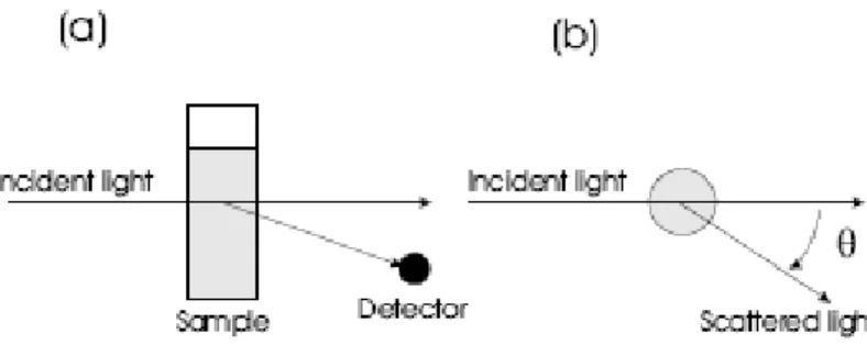
4.2.1.1. Static Light scattering 49

4.2.1.2. Dynamic light scattering 50

4.2.2. Experimental procedures 52

4.2.2.1 Light scattering 52

4.2.2.2 Preparation of α-crystallin suspensions 53

4.3. Experimental Results 53

4.3.1. Temperature dependence of nucleation and aggregation

kinetics 53

4.3.2. Ca2+ dependence of nucleation and aggregation

kinetics 59

4.3.3. Concentration dependence of nucleation and aggregation

kinetics 60

4.4. Discussion 61

4.4.1. Determination of nucleation and aggregation rates 61 4.4.2. Thermodynamic behaviour of nucleation and aggregation

Rates: evidence of a self-chaperone behaviour 65

5. CONCLUSIONS 77

Bibliography 81

1.Introduction

1.1.

Cataract

The eye and its architecture, at the macroscopic, microscopic and molecular level, is a nature’s masterpiece. Most impressive is the optical quality of the lens: the cones in the retina are visible through the intact optics of animal and human eyes (Hughes, 1996). The lens is a cellular organ and its transparency is due to its complex architecture and unique protein composition. Unfortunately, the delicate balance required for transparency is easily disturbed with lens opacity, cataract, as a result.

Cataract is the most common cause of blindness, and, therefore, of enormous medical and economical relevance worldwide. Ultimately, the only way to restore sight is cataract surgery. Current levels of surgery remain too low to tackle the backlog of cataract blind, estimated to be 16–20 million worldwide, and to reduce the rising world incidence due to the ageing population. The social impact and economic cost of cataract have motivated extensive research on the lens and an enormous amount of knowledge has been accumulated.

From the physicochemical point of view, the main cause for lens opacification is the condensation of eye lens proteins into randomly distributed aggregates with

average molecular masses beyond 50 MDa (Benedek, 1971, 1997). Unfortunately, the main cause of protein lens aggregation is still unknown. The causes of aggregation can be several: point mutations, disulfide bond formation, post-translational modifications leading to altered protein interactions, like deamidation and methylation (Hleon et al., 1999; Kmoch et al., 2000). An increasing number of diseases are believed to result from the aggregation of

misfolded proteins: a failure in the physical process by which a polypeptide folds

into its characteristic three-dimensional structure (protein folding), usually produces proteins with altered interactions that can lead to their multimerization into insoluble, extracellular aggregates and/or intracellular inclusions (Carrel, 1997; Dobson, 1999; Soto, 2001). Among these protein-misfolding diseases there are the Alzheimer’s disease (AD), Parkinson’s disease (PD), Huntington’s disease (HD) (and related polyglutamine disorders including several forms of spinocerebellar ataxia or SCA), transmissible spongiform encephalopathies (TSEs, which include several human and animal diseases) and amyotrophic lateral sclerosis (ALS). Despite their obvious differences in clinical symptoms and disease progression, they share some common features: kinetic studies have shown that the aggregation of A , PrP, huntingtin, -synuclein and other proteins involved in these diseases follows a nucleation mechanism (Jarret, 1993; Scherzinger, 1999; Wood, 1999) which resembles a crystallization process. The critical event is the formation of protein oligomers that act as a nucleus to direct further growth of aggregates. Nucleation-dependent aggregation is characterized by a slow lag phase in which a series of unfavourable interactions forms an oligomeric nucleus, which then rapidly grows to form larger polymers. The lag phase can be minimized or removed by addition of seeds (Dobson, 1999). Several studies showed how cataract could be considered among the protein misfolding diseases because, in stressful conditions, heat and Ca2+ decrease both secondary and tertiary–quaternary structure stability of the lenticular structural protein

α−

crystallin, having the

effect of a partial unfolding (Del Valle, 2001). But detailed characterizations of lens proteins aggregation kinetics are still lacking, although they are an important tool to distinguish whether cataract can be considered among the protein misfolding diseases, or among diseases involving altered protein interactions with native proteins.

Another important aspect being debated pertains the main cause of misfolding diseases. Environmental factors that might catalyse protein misfolding and the related pathologies include changes in ions like Ca2+, pH or oxidative stress, thermal stress, macromolecular crowding and increases in the concentration of the misfolded protein (Teplow, 1998). Among these, the prevalent hypothesis for protein folding diseases is that they result from an insufficiency in the protein chaperoning system of the cell: to ensure that cells and organisms function properly, the unfolding of cytoplasmic proteins evokes stress induced systems (heat shock responses) that inhibit general protein synthesis, and switch the resources of the cell to synthesizing protein chaperones, thus giving cells time and means to deal with the unfolded protein stress. The disease starts when the unfolded protein accumulates faster than the chaperoning system can deal with aggregating protein (Dobson, 1999; Csermely, 2001). It should be noted that among the most prominent cytoplasmic chaperones synthesized, like Hsp90, Hsp70 and the small heat shock proteins (sHsps), there is also α−crystallin. This should have an important protective role, because the lens cell lacks protein synthetic capacity and thus cannot increase its protein chaperone content when non-native protein starts aggregating. Therefore, in analogy with the protein misfolding diseases, the main cause for cataract could be that, with time, as lenticular proteins unfold, the chaperone capacity of α−crystallin will be exhausted and protein aggregates will be formed (Horwitz, 1992; Derham and Harding, 1999; Clark and Muchowski, 2000). Investigations on aggregation kinetics of α-crystallins in hyperthermic

and stressful conditions can be a valuable tool in searching if a protective mechanism exists, how it works, why and when it ceases to work .

1.2 Aim of this work

We have seen how a detailed characterization of the aggregation kinetics of the lens proteins allows to distinguish among the different molecular mechanisms responsible for their condensation.

Therefore, in this thesis we will report the aggregation kinetics of the lens structural protein α-crystallin followed in vitro, under physiological and paraphysiological conditions. Next, we will develop a quantitative kinetic model of the process that leads to the condensation of eye lens proteins into randomly distributed aggregates by means of population balance equations (PBE), combined with an extensive experimental investigation using light scattering in order to compute experimentally measured quantities.

The model describes the growth kinetics as a two step-process, a nucleation phase followed by an aggregation phase. This mechanism is a further evidence that cataract can be considered among the protein misfolding disease and is not an aggregation process due to altered native protein interactions.

Furthermore, for the first time we will verify how condensation of misfolded proteins does lead also to randomly distributed aggregates, and not only to fibrillization, through a nucleation mechanism, as hipotized by Dobson (Dobson, 1999). This means that nucleation, rather than fibrillization, is a common feature of the misfolding diseases.

Last, but not least, we will find evidence that the α-crystallin exhibits a temperature-dependent protective effect towards self-aggregation, which preserves the lens from a premature opacification by delaying the aggregation of denatured crystallins in hypertermic and stressful conditions. A possible mechanism explaining this effect will be given on the basis of the available

experimental data. This peculiar response to external insults it has been investigated in vitro and it could be directly related to the response expressed in

vivo, because the lens fibre cell represents a special case of aged cells,

characterized by a complete lack of an heat shock system except for one component, α-crystallin.

2. Structure of crystallins

2.1 Lens differentiation: structuring a tissue for

transparency

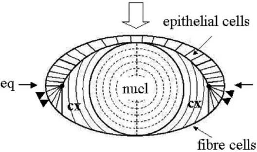
The lens is a focusing device that allows images to be formed on the retina. To serve this function, the eye lens has to fulfil two requirements; it has to provide transparency and a high refractive index, i.e. low light scattering and high solubility of its cytoplasmic proteins, the crystallins. From the physical point of view, transparency is limited by absorption and scattering of visible light. In the cataract-free lens, absorption in the visible wavelength range is negligible. The cellular structure of the lens can meet these biophysical requirements because of its unique morphology and composition. In the mature lens, hexagonally packed, long ribbon-like fibre cells, which in man are up to 10 mm long, are arranged in concentric shells, with the oldest cells at the centre and the youngest on the outside (Fig. 1). The shape of the fibre cells is determined and maintained by an extensive cytoskeleton. The lens fibre cells have an unusually high protein content: the soft ovoid human lens has a protein concentration around 0.32 g/ml. The abundant water-soluble crystallins account for most of the lens fibre cell protein.

Light scattering may originate from the differing refractive indices of the membrane and the cytoplasm of the fibre cells, particularly in the cortex (Michael et al., 2003). The experimental evidence for this refractive index difference is clearly seen in the diffraction peaks recorded when laser light is passed through a thin peripheral section of the lens (Benedek, 1979). The absence of diffraction when light is directed along the optical axis is presumably a consequence of the continuous gradual change in orientation between layers of cells along this axis. In the centre of the lens, the refractive index of the membranes is the same as that of the cytoplasm and the orientation of the membrane is of lesser importance (Michael et al., 2003). The lens is determined during early embryonic development (Grainger, 1992) and derives from the ectoderm overlaying the optic cup. The surface ectoderm cells invaginate to form the lens vesicle with cells on the posterior side elongating to primary lens fibre cells filling the vesicle space. Cells on the anterior side remain a monolayer of epithelial cells, with their basal side facing outward and the apical side facing towards the lens fibre cells (Fig. 1).

FIGURE 1. Schematic drawing of a sagittal section through a vertebrate lens. The monolayer of epithelial cells and the fibre cell mass are indicated. The direction of incident light and the optical axis is represented by the open arrow; the equatorial plane by the two single arrows. The arrowheads show the region where the epithelial cells differentiate to secondary fibre cells. nucl: the nuclear region; cx: the cortical region, eq: the equatorial region.

Lens epithelial cells divide in a region just anterior to the equator, the cells at the equatorial zone elongate to form secondary fibre cells which form a continuous layer overlaying the primary fibres (Bron, 2000). During differentiation of the fibre cells, the different classes of crystallin genes are expressed in a strict temporal and spatial order. Furthermore, the expression of the crystallin genes is regulated in a developmental manner, with some of the crystallins being expressed primarily in the foetal lens, others only later. Crystallins synthesized during early development will be located in the core of the mature lens; crystallins expressed during later development will abound in the cortex. The design principle of vertebrate lenses is thus one of deposition of complex mixtures of crystallins that vary in their relative proportions along the optical axis and the equatorial plane, put in place by differential gene activity during development. As the last step in differentiation, fibre cells lose their nuclei, mitochondria and ribosomes in a process resembling the early steps of apoptosis (Bassnett, 2002). This loss of cellular organelles is required for transparency but has as consequence that the terminally differentiated fibre cell can no longer synthesize or degrade proteins. Hence, lens proteins that are located at the centre of the lens, and synthesized during foetal development, cannot be replaced and must last for the whole lifetime of the organism.

2.2. The crystallins

The abundant soluble proteins of the vertebrate eye lens are collectively known as the crystallins (Table 1). All vertebrate lenses examined contain three classes of crystallins, the α-, β- and γ-crystallins, also known as the ubiquitous crystallins, although in widely varying ratios. Using a mixture of different sized protein assemblies to fill the lens fibre cells insures polydispersity and prevents crystallization.

In order to fulfil their optical function, crystallins have to be first and foremost soluble. As they have to last the whole life span of the organism they must also be stable.

ARTICLE IN PRES

2.3

The

α-crystallins

2.3.1 Primary, secondary and tertiary structure

There are two α−crystallin genes, αA and αB, encoding proteins that share around 60% sequence identity (Bloemendal and de Jong, 1991). αΑ−crystallin is the lens-specific member of the family. In fact, only traces of it are found in some other tissues (Srinivasan, 1992). On the other hand, αΒ−crystallin is more widely expressed, and particularly abundant in brain, heart and muscle (Iwaki, 1990). In man, the ratio of αA- to αB-crystallin in the foetal lens is about 2:1 and the ratio decreases to about 3:2 in the water-soluble fraction of a lens from a 54/55 year old (Ma, 1998). The α-crystallins are presumed to function both as structural proteins and as chaperones in the lens (see section 2.3.3)

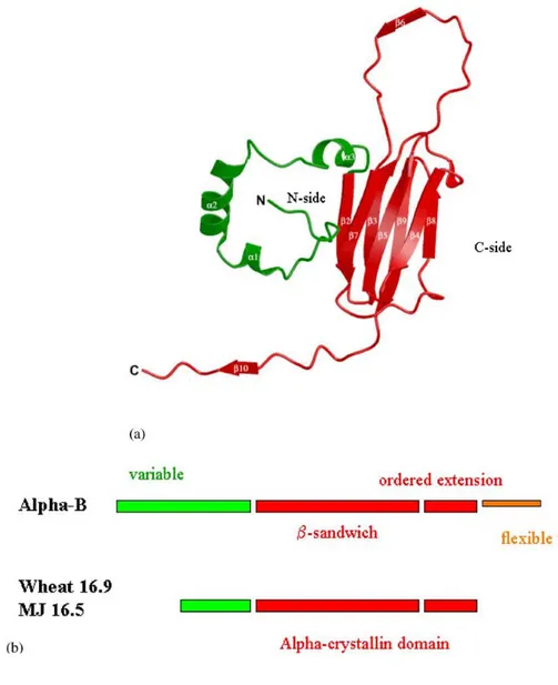
CD- and IR-based secondary structure predictions for the α-crystallin subunit suggested predominantly β-sheet and less than 20% helix content. Due to the polydisperse size distribution of both the natural and recombinant protein, crystallization of vertebrate α−crystallin has been unsuccessful so far. Thus, neither the detailed 3D structure of the subunit nor the topology of the subunit assembly is presently known. It is only known from their primary structure that both α-crystallins contain a particular amino-acid sequence called the ‘‘α-crystallin domain’’ shared by all the members of the sHsps (de Jong, 1998): sHsp sequences are characterized by a C-terminal ‘‘α−crystallin domain’’ linked to a variable N-terminal region (de Jong, 1998). It was proposed that the ‘‘α−crystallin domain’’ might resemble an Ig fold (Mornon, 1998). This hypothesis was confirmed when the 2.7 Å X-ray structure of an ‘‘α−crystallin domain’’ was solved from an the first sHsp assembly from a higher organism, wheat (van Montfort, 2001).

FIGURE 2. Structure of a wheat small heat shock protein (based on Fig. 2 from van Montfort et al., 2001). (a) Ribbon diagram of the protein with the N-terminal arm shown in green, the α-crystallin domain and C-terminal extension in red with the N- and C-termini, and secondary structure elements labelled. (b) The conserved α-crystallin domain as recognized by sequence profile searches is shown in red. It comprises two structural modules, the β-sandwich and the ordered extension. The hinge connecting these two modules is flexible allowing different assemblies. The flexible tail is shown in orange and corresponds to the regions classed as mobile when the assembly is investigated by NMR spectroscopy. The N-terminal regions (green) are variable in length and sequence.

Looking in detail at one monomer of this sHsp (Fig. 2a), the domain fold is seen to be composed of a two sheet β−sandwich structure surrounded by ‘‘loose ends’’, in contrast with the neat arrangement of strands in the βγ−crystallin domain (see section 2.4). This is considered to represent an ‘‘unfinished domain’’, as the edges of both sheets on the two sides of the sandwich (labelled

domain’’ in the α−crystallins is likely to have the β−sandwich fold in which the C-side protection is provided by an ordered extension of a partner subunit. The α−crystallins also have an additional C-terminal tail for which there is evidence of conformational flexibility (Fig. 2b).

2.3.2 Quaternary Structure

Vertebrate α-crystallins, like many sHsps, form polydisperse multimers (MacRae, 2000). α−Crystallins have molecular masses between 300 and 1200 kDa, depending on the solvent conditions and other variables. These multimers contain about 40 subunits of αΑ− and αΒ−crystallin in a ratio of 3 to 1 (for review, see Horwitz, 2003). α−Crystallin can be readily denatured by heat and Ca2+, following pathways that include both changes in the secondary structure and the state of assembly (Doss-Pepe, 1998; Putilina, 2003).

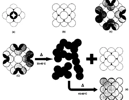
To monitor the heat-induced changes that occur in the structural domain of lens α-crystallin diverse techniques like circular dichroism, fluorescence, differential scanning calorimetry, were used (Tardieu, 1986; Walsh, 1991). Based on these results a model is proposed by Tardieu (Tardieu, 1986) and extended by Walsh (Walsh, 1991). The proposed model of native α-crystallin has a three-layer structure in which the inner layer (core) is a micelle containing 12 subunits arranged as a cuboctahedral symmetry (fig. 3a). The apolar region is directed inward constituting a hydrophobic core similar to a micelle and adding structural stability. A second layer of six subunits has similar but not identical structure to the first layer, directing its apolar face toward the hydrophobic core (fig. 3b). Thus, these two layers constitute a micelle-like structure with octahedral symmetry. The third layer adds more subunits for a total of not more than 42 (Fig.3c). The inner two-layer structure of molecular mass 360 kDa is highly stable called αΜ. The three-layer structure of the native protein, instead,

layers, and at higher temperatures (45-60°C) rapidly reassociates to a slightly modified two-layer structure with a stability similar to that of αΜ (Fig. 3d). The

proposed model does not require any specific assembly of the αA and αB subunits in each layer, but the fluorescence results suggest that the native inner two layers probably contain mostly αA.

FIGURE 3. Schematic representation of the proposed model. (a) the first, innermost layer consists of 12 subunits (b) first and second layers comprise a total of 18 subunits, arranged as a cuboctahedral symmetry. (c) first, second, and third layers comprise a total of 42 subunits, cuboctahedron type. The hydrophobic portion is shown in black. (d) a two-layer structure, similar but not identical to (b), formed upon heating the original three-layer structure (c).

Also Ca2+ alters the structural stability of α-crystallin leading to the formation of aggregates. Ca2+-induced aggregation of lens α-crystallin was initially studied by sedimentation analysis (Jedziniak, 1972) and the possible role for Ca2+ in the cataractogenesis process was discussed (Jedziniak, 1983; Duncan, 1984). Indeed, In human lenses with dense, highly localised opacities, Ca2+ distribution is not uniform and is highest in regions that scatter most light (Duncan, 1977). Recently, it was found that γ−crystallin from bovine lenses shows significant calcium-binding ability (Rajini, 2001), the greek key βγ−crystallin fold (see section 2.4) being the calcium-binding motif. The effect of Ca2+ on the thermal stability of α−crystallin by UV and Fourier-transform

cases, a Ca2+ -induced decrease in the midpoint of the thermal transition is detected. The presence of high [Ca2+ ] results also in a marked decrease of its chaperone activity in an insulin-aggregation assay. The results obtained from the spectroscopic analysis, and confirmed by circular dichroism (CD) measurements, indicate that Ca2+ decreases both secondary and tertiary– quaternary structure stability of α−crystallin. It is concluded that Ca2+ _{alters the}

structural stability of α-crystallin, resulting in impaired chaperone function and a lower protective ability towards other lens proteins, playing in that sense a role in the progressive loss of transparency of the eye lens in the cataractogenic process.

2.3.3 Lens α-crystallins and chaperone function

Like the α-crystallin, the other sHsps usually associate into high molecular weight monodisperse or polydisperse oligomers, able to protect against stress through the binding of a variety of partially unfolded substrates. α−Crystallin was demonstrated by Horwitz (Horwitz, 1992) to exhibit such chaperone properties in vitro. On the basis of these results, Horwitz proposed that α−crystallin would bind β−crystallin or γ−crystallin at the onset of their denaturation, thus preventing further precipitation and lens opacity.

The chaperone-like activity of α-crystallin depends on temperature (Raman and Rao, 1997). It is less pronounced below 30 °C and is enhanced above this temperature. The transition above at nearly 45 °C already investigated by Walsh, involving a quaternary structural transition and an enhanced or reorganized hydrophobic surfaces of α-crystallin, probably forms a part of the general mechanism of the chaperone function that is required more effectively in hypertermic and stressful conditions for the lens cell.

2.4

The

β- and γ-crystallins

The β−crystallins are a family of basic (βΒ1, βΒ2, βΒ3) and acidic (βΑ1, βΑ2, βΑ3 and βΑ4) polypeptides (Herbrink et al., 1975; Berbers et al., 1984). The sequences of their corresponding globular domains exhibit between 45 and 60% identity with each other, and about 30% with γ−crystallins.

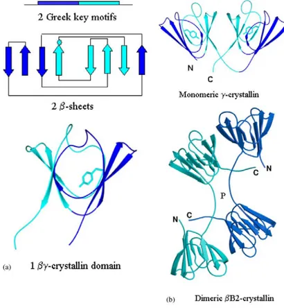
The oligomeric β− and the monomeric γ−crystallins are both built up out of four “Greek key” motifs organized into two domains. This common secondary structural motif has the typical shape of Attic vases (Fig. 4a).

FIGURE 4. The modular structure of the βγ-crystallins. (a) Each βγ-crystallin domain is made from two linear sequence related Greek key motifs that intercalate on folding to form two β-sheets. The second motif (shown in turquoise) is more sequence conserved among family members and contains a tyrosine corner positioned between the 3rd and 4th β−strands (indicated by the turquoise filled circle). The two sheets form a compact and pseudo-symmetric βγ-crystallin domain. (b) All lens βγ-crystallins comprise two domains. In the monomeric γ-crystallins the N-and C-terminal domains pair in a symmetrical manner about an approximate dyad using mainly residues from motifs 2 and 4. In the dimeric βB2-crystallin, the N-terminal domain pairs with the C-terminal domain of the partner subunit, in a process known as domain swapping.

The two consecutive Greek key motifs comprising eight β−strands intercalate to formtwo β−sheets that pack together to form a β−sandwich domain.

Although β−sandwich domains are common in proteins, in βγ−crystallins they are characterized by an high internal conformational symmetry and by a conserved folded hairpin structure for each motif. Sequence–structure alignment of all the Greek key motifs shows that two quite distal residues, a glycine and a serine, are the most conserved and are involved in stabilizing the supersecondary fold by packing this β−hairpin over the β−sheet (Blundell et al., 1981).

FIGURE 5. Structural polydispersity in the lens crystallins. The lens αβγ-crystallins constitute an array of differently sized proteins. Although the γ-crystallin family members are individually monodisperse, the oligomeric crystallins have the potential of greater polydispersity. In the case of dimeric β-crystallins, not only is there a potential combinatorial diversity due to the identity of monomer components, but also the possibility of conformational diversity generated through use of interface selection in subunit pairing. This diversity can then only be increased in the higher order β-crystallin assemblies, although little precise information is available about them. In the case of α-crystallin, not only is there the potential for diversity in the location of the αA- and αB-crystallin subunits in the assembly, there is also evidence for variation in the number of assembly subunits. The α-crystallin cartoon is based on the model of heteromeric lens α-crystallin by Tardieu and colleagues (Tardieu et al., 1986).

The main sequence difference between monomeric γ-crystallins and oligomeric β-crystallins is the presence of sequence extensions in the oligomers which permits the linkage between monomers (Fig. 4b). The βγ−crystallin domain system is thus certainly versatile in terms of domain assembly and may well have evolved to generate conformational and combinatorial diversity in the oligomeric β−crystallins. Not only might this be a device for inhibiting crystallization at the high protein concentration of the lens, but it could also contribute to forming a range of oligomeric sizes. In turn these contribute to an even protein distribution and refractive index (Fig. 5). Although higher assemblies of β−crystallins can be made in vitro, the size reached is not yet as large as the in vivo assemblies.

I

3. Modeling nucleation-aggregation

kinetics

3.1 Colloidal systems and protein systems

Colloidal science has advanced to a great extent over the last forty years being inspired by and inspiring applications. The large variety of colloidal systems that can be prepared or found in nature provide rich possibilities to gain insight into phenomena and processes of interest to physicists, chemists, biologists, material and environmental scientists, and engineers. This explains the broad spectrum of papers published on the various aspects of colloidal science.

The kinetics of aggregation has been a topic of scientific efforts since the pioneering work of Marian von Smoluchowsky at the beginning of the previous century (von Smoluchowky, 1917). He derived the first aggregation rate constants for systems where only Brownian forces cause the motion of the particles and the collisions between them. He considered the case where the particles are completely destabilized and their interactions are dominated only by attractive forces, resulting in the formation of a new cluster upon any

collision between two particles. This constitutes the fastest aggregation rate possible. The aggregation kinetics of particles that are not fully destabilized but retain some repulsive forces in addition to the attractive ones, has been described by Fuchs almost 20 years later (Fuchs, 1934). He introduced the concept of a relative aggregation rate, given as the ratio of the fastest aggregation rate derived by Smoluchowsky to the one observed in only partially destabilized systems. This important parameter for colloidal science is called the

Fuchs stability ratio. Later the Derjaguin-Landau-Verwey-Oveerbek theory

(DLVO) has been overly successful in providing a qualitative and to some extent even quantitative framework to calculate the stability ratio (Verwey, 1948; Derjaguin, 1989; Bostrom, 2001). Their work breeded the concept of population balance equations which has been used in many applications in order to model distributed particulate populations and the changes they undergo as a function of time or other system variables (Ramkrishna, 2000). The population balance equations (PBE) for aggregation form the basis of the investigations presented in this thesis.

Besides the colloidal stability, the structure of aggregates evolving in colloidal dispersions of small particles has long puzzled scientists due to its seemingly complex nature. Mandelbrot, with his breakthrough concept of fractal geometry (Mandelbrot, 1982), sparked renewed interest in colloidal aggregation by providing a framework which allowed to characterize the random structure of an aggregate in an average way by a simple power-law relation between its mass and radius, i R∼ df , where i is the number of particles in a cluster and R its radius (Forrest, 1979; Witten, 1981).

The exponent df, the fractal dimension, can be used to describe how open or

dense a certain aggregate is. This exponents takes values smaller than three and therefore fractal aggregates are characterized by a density decreasing with increasing number of particles in the cluster.

Later, in a series of hallmark papers, Lin et al. (Lin, 1989; Lin, 1990) have shown by using dynamic and static light scattering that colloidal aggregation exhibits two universal limits: these are diffusion limited colloid aggregation (DLCA), characterized by a complete destabilization of the colloidal particles with aggregation taking place upon every collision, and reaction limited colloid aggregation (RLCA), where some remaining repulsive electrostatic forces allow only a small fraction of collisions to result in the formation of a new aggregate. The structure of the aggregates in DLCA is rather open and fractal dimensions of df ~ 1.8 have been found both in experiments and computer simulations

(Odriozola, 1999). Depending on which aggregation model is used to simulate DLCA, two kind of shapes of the cluster mass distribution (CMD) are predicted. When using a constant aggregation kernel, the predicted CMD is rather flat (Lin, 1990). However, when properly accounting for the size dependence of the aggregation rate constant, the predicted CMD exhibits a bell shape, which differs from the previous one in the smaller aggregate size region (Odriozola, 1999). Both these CMDs in DLCA have a sharp cut-off at a certain mass, which itself grows with a power law behaviour in time (Lin, 1990).

The lower sticking probability in RLCA results in denser aggregates with df ~

2.1, which was also confirmed in experiments and computer simulations (Lin, 1990). The CMD in RLCA is characterized by a power law shape with an exponent

τ

c = 1.5 and a sharp cut-off. Here, the cut-off mass grows

exponentially in time (Lin, 1990). Importantly, Lin et al. demonstrated that these regimes exist for different colloidal systems (gold, silica and polystyrene).

Since then, the aggregation kinetics of several different colloidal particle systems has been studied in dilute conditions. Among these systems, charge stabilized polystyrene latexes in aqueous solution play an important role as model systems. In particular, the stability behaviour of polystyrene spheres with different charged functional groups as a function of electrolyte concentration, pH and the amount of additional charged and/or steric surfactant has been

analyzed in detail (Behrens, 2000; Peula, 1998, Sefcik, 2003; Romero-Cano, 1998, Porcel, 2001).

Also biological systems like globular proteins or milk are often analyzed in the framework of aggregation discussed above (Weijers, 2002; Durand, 2002). The aggregation behaviour observed in all of these systems is often compared to the classification given by the limiting regimes, i.e. DLCA and RLCA. The supramolecular aggregation of α-crystallin, induced by generating heat-modified α-crystallin forms and by stabilizing the clusters with calcium ions, was investigated by means of static and dynamic light scattering by our group (Andreasi Bassi et. Al, 1995). The kinetic pattern of the aggregation and the structural features of the clusters can be described according to the RLCA model previously adopted for the study of colloidal particles aggregation systems. The structure factor of the clusters is typical of fractal aggregates. A fractal dimension df =2.05 was determined, indicating a low probability of

sticking together of the primitive aggregating particles.

The conclusion of the foregoing discussion is that various aggregation mechanisms and cluster structures have been observed in a variety of colloidal and biological systems. However, the application of colloidal aggregations theories to proteins systems is often insufficient because it lacks the modelization of diverse protein related phenomena, like nucleation and unfolding. The importance of knowing unfolding, nucleation and aggregation rates in protein folding diseases requires a detailed model accounting for the unfolding process and the nucleation process.

Furthermore, a systematic comparison of the corresponding CMD obtained by solving the PBE, with an appropriate experimental characterization of the CMD, is still missing. This experimental characterization of aggregation in the sub-micron size range relies primarily on static and dynamic light scattering techniques (Lin, 1990; Sorensen, 2001), which consequently requires a detailed model for light scattering to calculate these quantities from the PBE.

The cluster mass distribution (CMD) and the aggregate size distribution, which obviously depend crucially on the processing conditions, in fact completely characterize the aggregation process.

3.2 Aggregation kinetics in colloidal systems

3.2.1 Population balance equation

Population balances (PBE) are general conservation laws applicable to a variety of particulate systems (Ramkrishna, 2000). Aggregation in homogeneously mixed colloidal dispersions can conveniently be described by PBE, where we use mass as the internal coordinate for representing aggregates undergoing birth and death events. These events lead to the formation and disappearance of aggregates of mass m and indicating with ni (t) the number of aggregates of mass

m=i m0 at time t we obtain the following form of the population balance:

, 1 1 1 ( ) ( ) ( ) ( ) ( ) 2 s i i j j i j j i i j j j n t K₋ n₋ t n t n t ∞ K n t = = =

∑

−

∑

, j (3.1)

where the two terms on the right-hand side represent the rate of birth and death of units of mass m=i m0 per unit volume, respectively. The first one represents

the production of aggregates of mass m=i m0 by aggregation of two smaller

aggregates of mass and m′ m m′− , while the second considers the loss of particles of mass m due to aggregation with any other aggregate of mass m′. The aggregation frequency function accounts for two physical factors, which constitute the aggregation process: the collision frequency between two particles and the corresponding sticking efficiency.

, i j

K

The validity of the PBE in the form of equation (3.1) relies on several assumptions. In particular, in concentrated systems it can be expected that more than two particles undergo aggregation simultaneously and that the presence of surrounding particles influences the two aggregating ones. On the other hand, in

equation (3.1) only binary aggregation events are considered. The pair probability function p m m t₂( , , )′ which accounts for the probability of finding two particles of mass m and m’ undergoing aggregation at the same spatial location in the time interval fit, is computed by assuming an independent probability of finding each of the two involved aggregates in the system, i.e.

2( , , ) 1( , ) ( , )1

p m m t′ = p m t p m t′ . This assumption is known as the closure hypothesis and has been discussed in the literature (Ramkrishna, 1976).

At the other extreme of diluted systems, where the population is constituted by only a few particles, it has been shown that the PBE (3.1) fails and single statistical events become important (Sampson, 1985). This is due to the fact that in diluted systems the few particles present are correlated, meaning that the relation p m m t2( , , )′ = p m t f m t1( , ) ( , )1 ′ fails and higher order product density

functions 2

( , , ),

3

( , ,

, ),...,

( , ,

,....,

, )

M M

p m m t p m m m t

′

′ ′′

p m m m

′ ′′

m t

have to be used in addition to the first-order functions used in equation (3.1).

No attempt is made in the following to a priori determine the upper and lower concentration bounds, where the aggregation PBE in the form of equation (3.1) is accurate. This would not be a straightforward task and therefore we ultimately rely on the comparison with experimental data.

3.2.2 Numerical solution and reconstruction of the CMD

The description of aggregation phenomena in the framework of population balances requires the coverage of several order of magnitudes in aggregate size. Primary particles in colloidal dispersions usually are in the size range of 5 - 500nm. Aggregation of these particles frequently results in clusters up to the size of 300 μm. Under certain operating conditions the formation of coagulum can occur, the radius of which can attain values up to 1 - 100mm.

Accordingly, in order to describe the evolution of the CMD over the whole range of particle and aggregate sizes, a simple linear discretization technique would result in a number of coupled ODE's not solvable in reasonable computer time. Thus, the application of a geometric or other expanding grids for the representation of particle sizes is indispensable for computational efficiency. A widely used method of approximation is the Runge-Kutta method (Forsythe, 1977). It uses a sampling of slopes through an interval and takes a weighted average to determine the right end point.

We implemented a homemade software with Labview 7.1, that uses this method to solve PBE systems of non-linear differential equations.

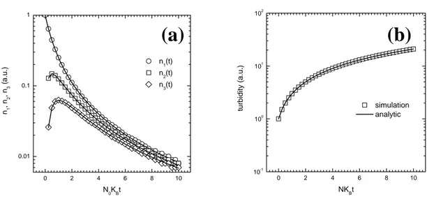
0 2 4 6 8 10 0.01 0.1 1 n1 , n 2 , n 3 (a .u .) N₀K_Bt n₁(t) n₂(t) n 3(t) 0 2 4 6 8 10 10-1 100 101 102 tu rbidit y (a. u .) NK_Bt simulation analytic

(a) (b)

FIGURE 6. Comparison between the analytical (Eq. 2.2) and the numerical RK solution for equation(3.1) with the constant kernel Ki, j = KB. (a) Discretized analytical solution for n1(t), n2(t) and n3(t) (solid line) and KR numerical solution; (b) continuous analytical solution for τ =

∑

_ii n2 i (solid line). and reconstructed numerical KR solution.

One important oft-neglected aspect is the reconstruction of the continuous distribution from the discretized one obtained from the RK method. To illustrate this point we consider the PBE (3.1) with a constant aggregation kernel, i.e.

,

i j B

K =K , for which an analytical solution exists: 1

0 0 0

( ) ( ) (1i ) i

i B B

where ni denotes the number of clusters of a certain dimensionless mass i =

mi/m1, where mi is the mass of a cluster with i primary particles and m1 is the

primary particle mass. In Figure 6(a) the discretized solution for n1(t), n2(t) and

n3(t) obtained with the RK method is compared with the corresponding values

obtained using the analytical solution (3.2). It is seen that the obtained values are in satisfactory agreement, thus indicating that the numerical RK method provides reliable results. The next point is to compare a function of all the

ni(t)’s, for example an experimentally accessible quantity like turbidity

obtained with the RK method with the corresponding values obtained using the analytical solution (3.2). The obtained results are compared in Figure 6(b) and again the agreement is satisfactory, thus indicating that, although very simple, this reconstruction procedure provides reliable results.

2

i

ii n

τ =

∑

Another relevant point in computing CMDs numerically is that the size range for the problem on hand has to be specified “a priori” by an upper and a lower bound, here conveniently denoted in terms of aggregate mass m0 and mM,

where M denotes the number of pivots in the discretized interval of aggregate mass. It should be noted that if the aggregates grow to such an extent that they reach the upper bound, and this is allowed to undergo further aggregation, the generated aggregates would be lost since they would exit the discretized size range and consequently the mass of the dispersed phase would not be conserved. To avoid this, we have to close the boundary by a collective pivot (i.e. the largest size mM), which includes all aggregates larger than mM and is excluded

from the aggregation process. By properly applying this closure procedure, it is possible to satisfy the mass balance, which is particularly useful when dealing with systems that can produce aggregates of very large size, as in the case of polymer or colloidal gelation (Krall, 1998; Butte, 2002). However, this situation does not occur in any of the computations shown in this work and the last pivot always contains a negligible mass.

3.2.3 Characteristics of aggregate populations

In many applications one is interested in the size of the aggregates, expressed in terms of volume or radius. Since the PBE discussed above provides a cluster mass distribution (CMD), the question arises of how the mass of an aggregate can be related to its size. In the case of coalescing particles this is straightforward since the spherical shape is conserved upon aggregation. In the case of aggregates constituted of primary particles rigidly adhering at their surface contacting points, we obtain randomly shaped aggregates that are usually described through the fractal scaling relation (Sorensen, 2001):

, 1 f d g i i f p R m i k m R ⎛ ⎞ = = ⎜_⎜ ⎟_⎟ ⎝ ⎠ (3.3)

where df is the fractal dimension, m1 and Rp denote the mass and radius of a

primary particle, while mi and Rg, i those of an aggregate. The prefactor kf is a

constant of the order of unity (Sorensen, 1997). The radius of gyration Rg, i in

equation (3.3) is connected to the hydrodynamic radius Rh, i by a factor

β

i,

typically of the order of one depending on the fractal dimension df (Lin, 1990,

Wiltzius, 1987). , , h i i g i R R β = (3.4)

Having set a fractal dimension value, equations (3.3) and (3.4) provide the average aggregate radii Rg, i and Rh, i as a function of the corresponding mass mi.

In selecting a quantity to define the size of an aggregate it is convenient to adhere to quantities that can be measured experimentally. Accessible non-integer moments of CMD are the radius of gyration 2

g

R

< > when using static light scattering (SLS), and the mean hydrodynamic radius , when using dynamic light scattering (DLS). In order to compare these experimental values with the cluster mass distribution n

,

h eff

R

< >

>

i, obtained from equation (3.1), we need to

relate the averages 2 and

g

R

the corresponding radii of the individual aggregates of mass i, given by Rg, i and

Rh, i . In the case of the radius of gyration, which relates to the mass distribution

inside the aggregate, such a relation is simply given by (Pusey, 1987)

2 2 , 2 2 i g i i g i i i n R R i n < >=

∑

∑

(3.5)

In the case of the hydrodynamic radius, which actually reflects the diffusion of the aggregate, the corresponding relation is more complex since it has to account for the effect of the measurement angle, the aggregate structure and the complex diffusion processes of the aggregates (Lin, 1990; Pusey, 1987):

2 , 2 1 , ( ) ( ) i i i h eff i i h i i i n S q R i n S q R− < >=

∑

∑

(3.6)

where Si (q) represents the structure factor of the aggregates of mass i and Rh;i

his hydrodynamic radius . A third average of interest in this thesis is the average scattered intensity, measured by static light scattering, which is obtained by intensity weighted averaging of the individual cluster structure factors Si(q) by

2

( ) _{i i i}( )

I q = K

∑

i n S q (3.7)

Where K is a constant accounting for instrument specificities and for the ∂ ∂n c of the suspension. Among the various possibilities for computing the structure factors of individual aggregates (Sorensen, 1999) we have chosen the Fisher-Burford relation not only for its simplicity but also because it has been shown to be quite accurate for aggregates having fractal dimensions equal to about 2 (Sorensen, 2001). This is given by

2 2 , 2 ( ) 1 ( ) 3 f d i f S q qR d − ⎛ = +_⎜⎜ ⎝ g i ⎠ ⎞ ⎟⎟ (3.8)

where q denotes the scattering wave vector, given by the relation:

0 4 2 n q π sen ϑ λ ⎛ ⎞ = _{⎜ ⎟} ⎝ ⎠ (3.9)

Where n is the refractive index of the liquid medium,

λ

0 the wavelength of the

used light and θ the scattering angle.

The Kirkwood–Riseman theory has been used to derive an analytical formula for the evaluation of Rg, i and Rh, i of fractal clusters. The proposed

relation is based on knowledge of the particle–particle correlation function and can be applied to clusters containing any number of particles larger than 4. Consequently, we have used the following relation, recently derived using Monte Carlo simulations (by means of an off-lattice cluster– cluster aggregation algorithm) and valid for aggregates containing more than four particles (Tirado Miranda, 2003; Lattuada, 2003), 2 3 3 0 2 ( 2 ) 2 4 (2 ) ( ) _{2 4} exp 4 f f p nn p p p b p p b p d p d p for r R N r R for r R R a g r _{r for} R c r r for R γ δ π ξ + − < ⎧ ⎪ ⎪ _{− =} ⎪ ⎪⎪ = ⎨ _{< <} ⎪ ⎪ ⎛ ⎞ ⎪ _{⎛ ⎞} ⎜ − ⎟ > ⎪ _{⎜ ⎜ ⎟ ⎟} ⎝ ⎠ ⎪ _{⎝ ⎠} ⎩ R r R r R (3.10)

where Nnn is the average number of nearest neighbour particles, δ(x) is the Dirac

delta function, and a and b are two parameters describing the structure of the second coordination shell, while c, df, ξ, and γ represent an empirical constant

factor, the fractal dimension, the cut-off length, and the cut-off exponent, respectively. While the fractal dimension df is the same for all DLCA (equal to

1.85) and RLCA clusters (equal to 2.05), all the other parameters change as the number of particles in the clusters changes. For the cut-off length the following fractal scaling has been adopted,

1 f d p R i ξ α= (3.11)

where the constant

α

equals 1.45 and 1.55 for DLCA and RLCA clusters,

respectively. The behaviour of the parameters a, b, Nnn, and γ as a function of the

( ) ( ) ( ) n n i e F i d i e f − = − + (3.12)

where the empirical parameters d, e, and f take different values for the different parameters, as summarized in Table 2. These values have been obtained from the simulations performed by Tirado Miranda (Tirado Miranda, 2003).

The value of the constant factor c is

(

3 3

)

4 1 4 2 3 4 4 1 , f b b nn d f p inc p a i N b c d R R γ f d π π ξ γ γ ξ + + − − − − + = ⎛ ⎛ ⎞⎞ ⎛ ⎞ ⎛ ⎞_⎜ ⎛ ⎞ _⎟ ⎜ ⎟ Γ − Γ ⎜ ⎟ ⎜ ⎟ ⎜ ⎟ ⎜ ⎟ _{⎝ ⎠⎜ ⎜⎝ ⎠ ⎟⎟} ⎝ ⎠ _{⎝ ⎝} γ _⎠⎠ (3.13) table 2

The advantage of the developed piecewise expression for g(r) is that it describes quantitatively the behaviour of the first two coordination shells and of the fractal part. By substituting eq. (3.10) into the expression of the hydrodynamic radius of an aggregate _, 0 1 ( )4 p h i p iR R R g r πrdr ∞ = +

_∫

(

)

1 1 2 2 , 1 4 1 4 4 1 4 2 1 , 2 2 f d f p f b b nn h i p inc p d R d N a c R iR b R γ π π ξ γ γ ξ γ − − + + ⎡ _{⎛ ⎞ ⎛ − ⎞}⎛ ⎛_{⎛ ⎞ −} ⎞⎞⎤ ⎢ ⎜ ⎜ ⎟⎟⎥ = + + − + _⎜⎜ _⎟⎟ Γ_{⎜ ⎟} − Γ _{⎜⎜ ⎟ ⎟} ⎜ ⎟ + ⎢ _{⎝ ⎠ ⎝ ⎠⎝ ⎝⎝ ⎠ ⎠⎠}⎥ ⎣ ⎦ (3.14)

where Γ and Γinc are the Euler gamma function and incomplete gamma function,

respectively (Zhu, 1994). This formula makes it possible to calculate the value of the hydrodynamic radius of a fractal aggregate readily, once the parameters appearing in the correlation function are known.

The analytical formula for the evaluation of Rg, i is (Tirado Miranda, 2003),

(

)

2 2 2 2 5 5 , , 4 2 4 4 4 4 2 1 , 2 5 2 f d p b b p f g i g p nn inc p R _a cR d R R N i b i R γ π π ξ γ γ ξ + + + ⎛ ⎞ ⎛ + ⎞⎛ ⎛⎛ ⎞ + ⎞⎞ ⎛ ⎞ _{⎜ ⎜ ⎟⎟} = + _⎝⎜ + ₊ − ⎟_⎠+ _⎜⎜ ⎟_⎟ Γ⎜ ⎟_⎜ − Γ _⎜⎜ ⎟ _⎟⎟ ⎝ ⎠ ⎝ ⎠ ⎝ ⎠ _{⎝ ⎝ ⎠⎠} 2 p f R d γ (3.15)

where Rg, p is the primary particle radius of gyration (for a sphere ,

3 5

g p p

R = R ).

Substituting now in equations (3.5) and (3.6) and (3.7) the expressions of the gyration and hydrodynamic radii of the aggregates, Rg, i and Rh, i, given by

equations (3.14) and (3.15), we can compare the experimentally accessible quantities I(q), 2

g

R

< >and , with that computed from the cluster mass distribution n

,

h eff

R

< >

i by solving the PBE (3.1). It is worth nothing that the gyration and

hydrodynamic radii represent different non-integer moments of the CMD, and therefore provide information not only on the average value but also on the higher order moments of the CMD. Accordingly, comparison of calculated with experimental values of both 2

g

R

< >and <Rh eff, > is a challenging test for the

reliability of an aggregation kinetic, and therefore provides the possibility of discriminating among different kinetic models with respect to various aggregation conditions. In order to compute I(q), 2

g

R

< >and from the equations above we need to know the fractal dimension, d

,

h eff

R

< >

f . This quantity is

measurable from SLS (Lin, 1990), measuring the angular distribution of scattered intensity (See chapter 4, § 4.2.1)

3.2.4 Forms of the aggregation kernel

In this section we discuss kernel equations for diffusion limited (DLCA) and reaction limited (RLCA) cluster aggregation that have been presented earlier in the literature.

3.2.4.1 DLCA-kernel

In the diffusion limited aggregation regime every collision between aggregates or primary particles is successful. The first and basic aggregation kernel for DLCA, accounting for the diffusive mobility (Di + Dj ) and the collision cross

section (Ri + Rj) of aggregates, has been derived by Smoluchowsky (von

Smoluchowsky, 1917). The diffusion coefficient D can be related to the radius of an equivalent sphere by the Stokes-Einstein relation D1 =k TB /(6πηRp). Using

these relations and neglecting the size dependence of the aggregation rate by assuming equal sized particles, one obtains the constant aggregation kernel:

8 3 B B k T K η = (3.16)

To incorporate aggregate structure using the fractal concept, the aggregate size is assumed to scale with its mass according to equation (3.3). An equivalent scaling is assumed for the diffusion coefficient (Jullien, 1992), given

by

1 1

/ df

i

D D =i− . From these relations we obtain

1 1 1 1 1 ( )( 4 f f f ij B ij d d d d ij K K B with ) f B i− j− i j = = + + (3.17)

where BBij is the matrix representing the collision cross section and the mobility

of the two colliding aggregates. This kernel has been found to properly describe experimental data in DLCA (Lin, 1990).

3.2.4.2 RLCA-kernel

In RLCA only a fraction of collisions is successful in forming a new aggregate, due to the incomplete screening of the repulsive forces between particles. Considering primary particles, the reduced sticking efficiency due to repulsive forces and hydrodynamic interactions can be expressed by the Fuchs stability ratio (Melis, 1999), 2 2 2 ( ) B p V k T p R e W R d G h h ∞ =

_∫

h (3.18)

where G(h) accounts for squeezing of the fluid between two approaching primary particles, h is the center to center distance and V is the particle interaction potential. This expression of the stability ratio applies only for primary particles and not for aggregates, that are composed of many primary particles. It has in fact been verified experimentally that the reactivity of aggregates increases with their mass (Lin, 1990; Broide, 1990), and therefore an additional factor Pij has to be considered, leading to the following general RLCA

kernel:

1

ij B ij ij

K =W K B P− (3.19)

Let us review in the following the various RLCA kernels reported in the literature and recast them in the form introduced above. Using theoretical scaling arguments Ball et al. (Ball, 1987) concluded that the efficiency of aggregation is determined by the larger of the two aggregating clusters through a power

λ

. This parameter accounts for the increased aggregation efficiency of larger clusters due to a larger number of contact possibilities on their surface and it has been shown to be in the range λ∈[1, 1.1]The resulting kernel can be written in terms of Pij in equation (3.19) as follows:

max{ , } ij P k k i λ = = j (3.20)

Other authors (Family, 1985) used the product kernel, given by

( )

ij

P = ij λ (3.21)

to simulate the CMD by a Monte-Carlo technique in the RLCA regime. They compared the obtained results with those given by the dynamic scaling theory, where the CMD obtained by Monte-Carlo simulations is represented by a dynamic scaling form. Relating these results to the Smoluchowsky equation and using equation (3.21) they a found non-trivial behaviour. There it has been pointed out that the asymptotic expressions of the dynamic scaling theory might not provide the exponent

λ

sufficiently accurately. In RLCA experiments using silica (Axford, 1997), it has been found, that the value of

λ

can vary in the range [0, 36; 0, 495], depending upon the solution ionic strength. In a study using a stochastic simulation method (Thorn, 1994), which compare the results to dynamic scaling theory as well as to experimental data (Broide, 1990), several values of

λ

have been tested.The following kernel has been shown to reproduce correctly the general features of the mass cluster distribution,

1 _{( )}

ij B ij

K ₌W K B ij− λ _(3.22)

where W is the Fuchs stability ratio and λ = 0.4 (de Hoog, 2001).

3.3

Extension of the model to protein systems:

nucleation

As we stated in § 4.1, application of colloidal aggregation theories to proteins systems is often insufficient because it lacks the modelization of diverse protein related phenomena, like nucleation and unfolding. On the other hand, Kinetic studies have shown that the aggregation of proteins involved in these diseases follows a nucleation mechanism. In the next paragraph we present a brief description of the nucleation processes, and in the following one we will

develop a model that can account for the nucleation step in protein growth kinetics.

3.3.1 The Classical Nucleation Theory (CNT)

Nucleation is the process which starts a first-order phase transformation. It’s a process consisting of the formation of nuclei of the new phase in the bulk of another phase. It’s an activated process, as the growing nucleus of the new phase must overcome a free-energy barrier. It is the nucleus at the top of this barrier that determines the nucleation rate, with the rate decreasing exponentially as the barrier height increases. This makes the timescale for nucleation much larger than the characteristic time scale of the microscopic dynamics of the system. The basic physics of nucleation is best illustrated with the help of the classical nucleation theory (CNT) (Debenedetti, 1996; Oxtoby 1998; Garcia Ruiz, 2003). In homogeneous nucleation, CNT expresses the rate per unit volume kN as the product of an exponential factor and a pre-exponential

factor A

*

exp( / )

N

k =A −ΔG k Tb (3.23)

The exponential factor is _exp( *_{/ )} where

b

G k T

−Δ _ΔG* _{is the free energy cost of}

creating the critical nucleus, the nucleus at the top of the barrier. The physical meaning of A will be discussed extensively in section 4.3.2.

CNT treats the nucleus as if it were a macroscopic phase. If we restrict ourselves to the nucleation of one fluid inside the bulk of another phase, then the nucleus is spherical and its free energy has just two terms: a bulk and a surface term. If the nucleus has a radius R then the bulk term is the free energy change involved in creating a sphere of radius R of the new phase. The surface term is the free-energy cost of the interface at the surface of this sphere. Thus the free energy is 3 4 4 3 n G π R _{ρ μ π}R2 Δ = − Δ + γ (3.24)

where Δμ is the difference between the chemical potential of the phase where the nucleus is forming, and the chemical potential of the phase nucleating, γ is the interfacial tension, ρ_n is the number density of the nucleating phases. For nucleation from a dilute solution or suspension, the solution can be treated as an ideal gas and then Δμ/k T_B =ln(ρ ρ_b/ _co)=s where ρ_b and ρ_co are the number densities in the bulk phase in which nucleation is occurring, and at coexistence, respectively. The free energy at the top of the barrier, _ΔG*_{, is easily found by}

setting the derivative of

Δ

F to zero. Then we have

(

)

3 * 2 16 3 _n G π γ ρ μ Δ = Δ (3.25)

This occurs for a critical nucleus of radius

* 2 ( n ) R γ ρ μ = Δ (3.26) Knowing _ΔG* and *

R is therefore possible to determine γ and ρ μnΔ .

3.4 Nucleation-Aggregation

kinetics

3.4.1 Modeling the effect of nucleation

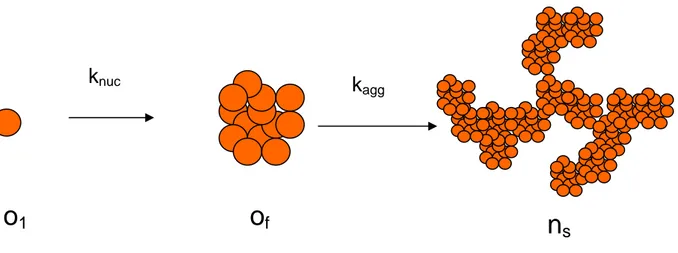
Kinetic studies have shown that the aggregation of proteins involved in protein folding diseases follows a nucleation mechanism, which resembles a crystallization process (see Figure 7). The critical event is the formation of protein oligomers that act as a nucleus to direct further growth of aggregates. Nucleation-dependent aggregation is characterized by a slow lag phase in which a series of unfavourable interactions forms an oligomeric nucleus, which then rapidly grows to form larger aggregates.

FIGURE 7 Schematic representation of the nucleation-aggregation process. The monomers o1 form protein oligomers of that act as a nucleus to direct the further growth of aggregates ns.

The aim of this section is to define a rigorous mathematical model that incorporates the physical chemistry of nucleation and the stochastic kinetics of aggregation and growth dynamics. A two-stage mechanism consisting of nucleation and stochastic aggregation is proposed.

The mechanism of nucleation is based on the Becker-Doring nucleation model from the field of atmospheric science (Seinfeld, 1998).

Accordingly (figure 7), the monomers o1, having mass m0, react with one another

as well as with different size oligomers so as to become larger clusters. The reactions between larger oligomers are negligible because their early concentrations and diffusivities are relatively low and small, respectively, as compared with the monomers. As oligomers grow, their chemical potentials drop, yet the surface tension to form new phases rises. Hence, there should exist a condition with minimum Gibbs free energy corresponding to the size of a cluster of (or nucleus), MC =Ncm0 (31). Any aggregates larger than the cluster

would convert into the basic unit of the aggregation. Therefore, indicating with

os(t) the number of the growing oligomer of mass m=s m0 at time t and

indicating with np(t) the number of the aggregates of mass m=p MC =p NC m0 at

time t, we obtain the following form of the population balance equations

o

1

knuc _k

agg

1 1,1 1 1 ,1 1 1 ,1 2 , , 1 1 , 1 1 ( ) ( ) ( ) ( ) ( ) ( 1) ( ) ( ) 1,..., 1 1 ( ) ( ) ( ) ( ) ( ) 2 ( 1) ( ) ( ) 1,..., C C C N N N N s s s s s j j C j p A A p p j j p j j p p j j j j N N j j N agg o t K o t o t o t K o t s o t K o t s N n t K n t n t n t K n t p K o t o t p N δ δ − − − = ∞ − − = = − − = − − − = = − + − =

∑

∑

∑

− (3.27)

where the two terms in the first equation on the right-hand side represent the rate of birth and death per unit volume of units of the nucleating oligomers, of mass

m=s m0, respectively. The nucleation frequency function , N i j

K

_{accounts for two}

physical factors which constitute the nucleation process: the collision frequency between two particles and the corresponding sticking efficiency. The two terms in the second equation on the right-hand side represent the rate of birth and death per unit volume of the aggregating clusters, of mass m= p MC =p NC m0,

respectively. The aggregation frequency function , A i j

K

_{accounts for the same}

physical factors proper of the nucleation process. The third term represents all the oligomers larger than the critical nucleus that are converting into the basic unit of the aggregation.

In the nucleation-aggregation model the averages 2

g

R

< >, and I(q) of the cluster mass distribution become

, h eff R < >

( )

2 _{2 2} 2 , , 2 2 2 p g p s g s p s g s p s p p n R s o R R s o p n ′ < >=

∑

+

∑

∑

∑

(3.28)

where R′_{g s,} and R_{g p,} are the corresponding gyration radii of the oligomers of mass s and aggregates of mass p,

( )

2 2 , ₂ 1 2 1 , , ( ) ( ) p p s p s h eff p p h p p s h s s p n S q s o R p n S q R s o R − − < >= + ′

∑

∑

∑

∑

(3.29)

where , are the corresponding hydrodynamic radii of the oligomers of mass s and aggregates of mass p, and S

,

h s

R′ R_{h p,}

p (q) represents the structure factor of the

(

2 2 2 2

)

0

( ) _s s C _p p p( )

I q =K m′

∑

s o +M

∑

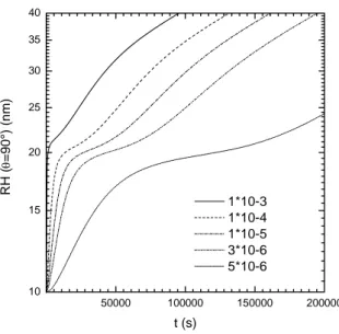
p n S q (3.30)

In figure 8 we show the trends of the simulated hydrodynamic radius obtained from (3.27) using (3.29) evaluated at q=193000 cm-1, and considering the first monomer o1(t) of 10 nm radius. The extended expressions for ,

N i j

K

_and , A i j

K

used are the sequent:

1 1 1 1 1 0.4 3 3 3 3 1 1 1 1 1 0.4 2.05 2.05 2.05 2.05 ( )( )( ) 4 ( )( ) 4 N N B ij A A B ij W K K i j i j ij W K ( ) K i j i j ij − _{− −} − _{− −} = + + = + + (3.31) With 1 N N B

k =W K− , ranging from 10-6 to 10-3 and 1 4

10

A A B

k ₌W K− ₌ − s−1_.

Therefore, in this simulation we consider both the aggregation and the nucleation process as an RLCA kinetic, but the structure of the critical nucleus is an hard sphere (df =3), and the structure of aggregates is a typical RLCA fractal

structure (df =2.05). 50000 100000 150000 200000 10 15 20 25 30 35 40 RH ( θ =90°) (nm) t (s) 1*10-3 1*10-4 1*10-5 3*10-6 5*10-6

FIGURE 8. simulated hydrodynamic radius obtained from the resolution of (3.34) using the expression (3.11) evaluated at q=193000 cm-1, and considering the first monomer o1(t) of 10

nm radius. The values for kN range from 10

-5 _{to 10}-3 _{and 3*10} 6 1

A