Planck 2015 results
Special feature
Planck 2015 results
XXVII. The second Planck catalogue of Sunyaev-Zeldovich sources
Planck Collaboration: P. A. R. Ade99, N. Aghanim68, M. Arnaud83, M. Ashdown79, 6, J. Aumont68, C. Baccigalupi97, A. J. Banday113, 10, R. B. Barreiro74, R. Barrena72, 43, J. G. Bartlett1, 77, N. Bartolo35, 76, E. Battaner116, 117, R. Battye78, K. Benabed69, 110, A. Benoît66, A. Benoit-Lévy27, 69, 110, J.-P. Bernard113, 10, M. Bersanelli38, 57, P. Bielewicz113, 10, 97, I. Bikmaev23, 2, H. Böhringer90, A. Bonaldi78, L. Bonavera74,
J. R. Bond9, J. Borrill15, 103, F. R. Bouchet69, 101, M. Bucher1, R. Burenin102, 92, C. Burigana56, 36, 58, R. C. Butler56, E. Calabrese106, J.-F. Cardoso84, 1, 69, P. Carvalho70, 79, A. Catalano85, 82, A. Challinor70, 79, 13, A. Chamballu83, 17, 68, R.-R. Chary65, H. C. Chiang30, 7, G. Chon90,
P. R. Christensen94, 42, D. L. Clements64, S. Colombi69, 110, L. P. L. Colombo26, 77, C. Combet85, B. Comis85, F. Couchot80, A. Coulais82, B. P. Crill77, 12, A. Curto6, 74, F. Cuttaia56, H. Dahle71, L. Danese97, R. D. Davies78, R. J. Davis78, P. de Bernardis37, A. de Rosa56, G. de Zotti53, 97,
J. Delabrouille1, F.-X. Désert62, C. Dickinson78, J. M. Diego74, K. Dolag115, 89, H. Dole68, 67, S. Donzelli57, O. Doré77, 12, M. Douspis68, A. Ducout69, 64, X. Dupac45, G. Efstathiou70, P. R. M. Eisenhardt77, F. Elsner27, 69, 110, T. A. Enßlin89, H. K. Eriksen71, E. Falgarone82, J. Fergusson13, F. Feroz6, A. Ferragamo73, 20, F. Finelli56, 58, O. Forni113, 10, M. Frailis55, A. A. Fraisse30, E. Franceschi56, A. Frejsel94, S. Galeotta55, S. Galli69, K. Ganga1, R. T. Génova-Santos72, 43, M. Giard113, 10, Y. Giraud-Héraud1, E. Gjerløw71, J. González-Nuevo74, 97,
K. M. Górski77, 118, K. J. B. Grainge6, 79, S. Gratton79, 70, A. Gregorio39, 55, 61, A. Gruppuso56, J. E. Gudmundsson30, F. K. Hansen71, D. Hanson91, 77, 9, D. L. Harrison70, 79, A. Hempel72, 43, 111, S. Henrot-Versillé80, C. Hernández-Monteagudo14, 89, D. Herranz74, S. R. Hildebrandt77, 12, E. Hivon69, 110, M. Hobson6, W. A. Holmes77, A. Hornstrup18, W. Hovest89, K. M. Huffenberger28, G. Hurier68, A. H. Jaffe64, T. R. Jaffe113, 10, T. Jin6, W. C. Jones30, M. Juvela29, E. Keihänen29, R. Keskitalo15, I. Khamitov107, 23, T. S. Kisner87, R. Kneissl44, 8,
J. Knoche89, M. Kunz19, 68, 3, H. Kurki-Suonio29, 51, G. Lagache5, 68, J.-M. Lamarre82, A. Lasenby6, 79, M. Lattanzi36, C. R. Lawrence77, R. Leonardi45, J. Lesgourgues108, 96, 81, F. Levrier82, M. Liguori35, 76, P. B. Lilje71, M. Linden-Vørnle18, M. López-Caniego45, 74, P. M. Lubin33, J. F. Macías-Pérez85, G. Maggio55, D. Maino38, 57, D. S. Y. Mak26, N. Mandolesi56, 36, A. Mangilli68, 80, P. G. Martin9, E. Martínez-González74, S. Masi37, S. Matarrese35, 76, 49, P. Mazzotta40, P. McGehee65, S. Mei48, 112, 12, A. Melchiorri37, 59, J.-B. Melin17, L. Mendes45, A. Mennella38, 57, M. Migliaccio70, 79, S. Mitra63, 77, M.-A. Miville-Deschênes68, 9, A. Moneti69, L. Montier113, 10, G. Morgante56, D. Mortlock64, A. Moss100, D. Munshi99, J. A. Murphy93, P. Naselsky94, 42, A. Nastasi68, F. Nati30, P. Natoli36, 4, 56, C. B. Netterfield22, H. U. Nørgaard-Nielsen18, F. Noviello78,
D. Novikov88, I. Novikov94, 88, M. Olamaie6, C. A. Oxborrow18, F. Paci97, L. Pagano37, 59, F. Pajot68, D. Paoletti56, 58, F. Pasian55, G. Patanchon1, T. J. Pearson12, 65, O. Perdereau80, L. Perotto85, Y. C. Perrott6, F. Perrotta97, V. Pettorino50, F. Piacentini37, M. Piat1, E. Pierpaoli26, D. Pietrobon77,
S. Plaszczynski80, E. Pointecouteau113, 10, G. Polenta4, 54, G. W. Pratt83, G. Prézeau12, 77, S. Prunet69, 110, J.-L. Puget68, J. P. Rachen24, 89, W. T. Reach114, R. Rebolo72, 16, 43, M. Reinecke89, M. Remazeilles78, 68, 1, C. Renault85, A. Renzi41, 60, I. Ristorcelli113, 10, G. Rocha77, 12, C. Rosset1,
M. Rossetti38, 57, G. Roudier1, 82, 77, E. Rozo31, J. A. Rubiño-Martín72, 43, C. Rumsey6, B. Rusholme65, E. S. Rykoff98, M. Sandri56, D. Santos85, R. D. E. Saunders6, M. Savelainen29, 51, G. Savini95, M. P. Schammel6, 75, D. Scott25, M. D. Seiffert77, 12, E. P. S. Shellard13, T. W. Shimwell6, 105,
L. D. Spencer99, S. A. Stanford32, D. Stern77, V. Stolyarov6, 79, 104, R. Stompor1, A. Streblyanska73, 20, R. Sudiwala99, R. Sunyaev89, 102, D. Sutton70, 79,?, A.-S. Suur-Uski29, 51, J.-F. Sygnet69, J. A. Tauber46, L. Terenzi47, 56, L. Toffolatti21, 74, 56, M. Tomasi38, 57, D. Tramonte72, 43, M. Tristram80, M. Tucci19, J. Tuovinen11, G. Umana52, L. Valenziano56, J. Valiviita29, 51, B. Van Tent86, P. Vielva74, F. Villa56, L. A. Wade77,
B. D. Wandelt69, 110, 34, I. K. Wehus77, S. D. M. White89, E. L. Wright109, D. Yvon17, A. Zacchei55, and A. Zonca33
(Affiliations can be found after the references) Received 5 February 2015/ Accepted 11 June 2015
ABSTRACT
We present the all-sky Planck catalogue of Sunyaev-Zeldovich (SZ) sources detected from the 29 month full-mission data. The catalogue (PSZ2) is the largest SZ-selected sample of galaxy clusters yet produced and the deepest systematic all-sky survey of galaxy clusters. It contains 1653 detec-tions, of which 1203 are confirmed clusters with identified counterparts in external data sets, and is the first SZ-selected cluster survey containing >103 confirmed clusters. We present a detailed analysis of the survey selection function in terms of its completeness and statistical reliability, placing a lower limit of 83% on the purity. Using simulations, we find that the estimates of the SZ strength parameter Y5R500 are robust to pressure-profile variation and beam systematics, but accurate conversion to Y500requires the use of prior information on the cluster extent. We describe the multi-wavelength search for counterparts in ancillary data, which makes use of radio, microwave, infra-red, optical, and X-ray data sets, and which places emphasis on the robustness of the counterpart match. We discuss the physical properties of the new sample and identify a population of low-redshift X-ray under-luminous clusters revealed by SZ selection. These objects appear in optical and SZ surveys with consistent properties for their mass, but are almost absent from ROSAT X-ray selected samples.
Key words. cosmology: observations – galaxies: clusters: general – catalogs
1. Introduction
This paper is one of a set associated with the 2015 Planck1full mission data release and describes the production and properties of the legacy catalogue of Sunyaev Zeldovich sources (PSZ2).
In the framework of hierarchical structure formation, peaks in the cosmological density field collapse and merge to form gravitationally bound halos of increasing mass (Peebles 1980). The galaxy clusters are the most massive of these bound struc-tures and act as signposts for the extrema of the cosmological density field on the relevant scales. The evolution of galaxy clus-ter abundance with mass and redshift is thus a sensitive cosmo-logical probe of the late-time Universe, providing unique con-straints on the normalization of the matter density fluctuations, σ8, the mean matter density, Ωm, the density and equation of
state of the dark energy field,ΩDEand w, as well as
constrain-ing some extensions of the minimal cosmological model, such as massive neutrinos, and non-standard scenarios such as modified gravity (see e.g.,Borgani & Kravtsov 2011;Allen et al. 2011). In recent years, cluster data from the microwave through to the X-ray parts of the spectrum have been used to constrain cos-mological parameters (Vikhlinin et al. 2009b;Rozo et al. 2010; Hasselfield et al. 2013;Benson et al. 2013;Planck Collaboration XX 2014;Zu et al. 2014).
Galaxy clusters are multi-component objects composed of dark matter, which dominates the mass, stars, cold gas, and dust in galaxies, and a hot ionized intra-cluster medium (ICM). These different components make clusters true multi-wavelength ob-jects. The galaxies emit in the optical and infrared. The ICM, which is the majority of the baryonic material by mass, emits in the X-rays via thermal bremsstrahlung and line emission, and energy-boosts cosmic microwave background (CMB) photons via inverse Compton scattering.
This last effect, the thermal Sunyaev Zeldovich (SZ) ef-fect (Sunyaev & Zeldovich 1970, 1980), imprints a redshift-independent spectral distortion on the CMB photons reach-ing us along the line of sight to the cluster. This results in an increase in intensity at frequencies above 220 GHz, and a decrease in intensity at lower frequencies. The Planck High-Frequency Instrument, HFI (Planck Collaboration VII 2016; Planck Collaboration VIII 2016), is unique in providing high-precision data for both the increment and the decrement across the whole sky.
The utility of a cluster survey for cosmological work depends on our ability to determine accurately its selection function and to obtain unbiased measurements of cluster mass and redshift. The first cluster surveys consisted of galaxy overdensities iden-tified by eye from photographic plates (Abell 1958). The con-struction of large optical catalogues improved significantly with the data from the SDSS (Koester et al. 2007), whose five pho-tometric bands have allowed robust phopho-tometric classification of red-sequence cluster galaxies and accurate photometric redshifts to z < 0.6 across 1/4 of the sky (Hao et al. 2010;Szabo et al. 2011; Wen et al. 2009; Rykoff et al. 2014). These catalogues now typically contain 104−105clusters and provide cluster
rich-ness as an observable that correlates with mass with an intrinsic scatter σintof about 25% (Rozo & Rykoff 2014).
1 Planck (http://www.esa.int/Planck) is a project of the European Space Agency (ESA) with instruments provided by two sci-entific consortia funded by ESA member states and led by Principal Investigators from France and Italy, telescope reflectors provided through a collaboration between ESA and a scientific consortium led and funded by Denmark, and additional contributions from NASA (USA).
Construction of X-ray cluster surveys is now a mature ac-tivity, with several catalogues available based on all-sky data from the ROSAT satellite, alongside additional catalogues of serendipitous detections from pointed observations (Ebeling et al. 1998;Böhringer et al. 2004;Reiprich & Böhringer 2002; Ebeling et al. 2010; Piffaretti et al. 2011;Burenin et al. 2007; Mehrtens et al. 2012). The most basic X-ray survey observ-able, the X-ray luminosity L500measured within r5002, has been
shown to correlate with mass, with an intrinsic scatter of about 40% (Pratt et al. 2009). Observables with lower intrinsic scatter against mass can be defined when pointed X-ray follow-up infor-mation is available, including the core-excised X-ray luminosity (Maughan 2007;Pratt et al. 2009) and Yx, the product of the gas
mass and the core-excised spectroscopic temperature (Kravtsov et al. 2006;Vikhlinin et al. 2009a;Mahdavi et al. 2013). While X-ray surveys are unique in their purity, they do, however, suf-fer from selection biases that favour low-redshift systems, due to flux limitations, and dynamically relaxed clusters with an X-ray bright cooling core (Eckert et al. 2011; Schuecker et al. 2003; Vikhlinin et al. 2009b;Chen et al. 2007).
SZ surveys offer a different window on the cluster pop-ulation: their selection function flattens towards higher red-shifts, providing a nearly mass-limited census of the cluster population at high redshift, where abundance is strongly sensi-tive to cosmological parameters (Carlstrom et al. 2002;Planck Collaboration XXIX 2014). The SZ survey observable is the in-tegrated Comptonisation parameter, Ysz, which is related to the
integrated electron pressure and hence the total thermal energy of the cluster gas. It is also expected to correlate with mass, with a low intrinsic scatter and little dependence on the dynamical state of the cluster (e.g.,da Silva et al. 2004;Kay et al. 2012; Hoekstra et al. 2012;Planck Collaboration Int. III 2013;Sifón et al. 2013).
The spherically-integrated pressure profiles of X-ray and SZ clusters have been observed to follow a near universal profile with little dispersion (Arnaud et al. 2010;Planck Collaboration Int. V 2013), permitting the detection of clusters with a matched multi-frequency filter based on some assumed pressure profile (Herranz et al. 2002; Melin et al. 2006). Samples constructed this way have well understood selection functions, though dis-crepancies due to profile mismatch or contaminating infra-red emission may still be present to some level. Large SZ surveys have only appeared recently, with catalogues of order 102 clus-ters released by the Atacama Cosmology Telescope (Hasselfield et al. 2013), the South Pole Telescope (Reichardt et al. 2013), and Planck satellite collaborations.
This is the third all-sky catalogue produced from Planck SZ data. The early Sunyaev-Zeldovich (ESZ) catalogue pre-sented 189 clusters detected from 10 months of survey data (Planck Collaboration 2011), while the PSZ1, the full-sky cata-logue assembled from the nominal mission data, presented 1227 cluster candidates detected from 15.5 months of data (Planck Collaboration XXIX 2014). This paper presents 1653 candidates detected from the full HFI mission survey of 29 months. 1203 of these have been confirmed in ancillary data, and 1094 have red-shift estimates. The PSZ2 expands the scope and sensitivity of the SZ view of galaxy clusters by substantially increasing the number of lower mass clusters available for study. It is also ex-pected to contain many new, as yet unconfirmed, high-redshift clusters. We report on the construction and characterisation of 2 The quantity r
500 is the cluster-centric distance within which the mean density is 500 times the critical density of the Universe at the cluster redshift.
ing redshifts. We also briefly discuss the physical properties of the sample.
This paper is organized as follows. In Sect.2we summarize the three extraction algorithms used to build the catalogue, fo-cussing on the changes in the algorithms since they were used to construct the PSZ1. In Sect.3we describe the construction of the catalogue. In Sect.4we present the survey selection func-tions (completeness and statistical reliability) and the comple-mentary approaches used to estimate them, while in Sect.5we discuss and validate the estimation of the Ysz parameters, both
blindly and when using prior information, and we compare the consistency of the new catalogue with the PSZ1 in Sect. 6. In Sect. 7 we report on the search for multi-wavelength counter-parts in ancillary catalogues and follow-up observations. Finally we present the physical properties of the sample in Sect.8and conclude in Sect.9. AppendixAsummarizes new high-z SDSS redshifts. AppendicesB,C, andEpresent a detailed account of the changes with respect to the PSZ1 in terms of redshift as-signments, detection code implementations, and missing PSZ1 detections, respectively. A full description of the available data products is given in AppendixD. All the data products can be obtained from the Planck Legacy Archive3.
2. Extraction algorithms
The SZ detection and parameter estimation algorithms used to construct the PSZ2 extend and refine those used to con-struct the PSZ1. In this section we recall the principles of the three algorithms. The refinements of each algorithm since the PSZ1 release are detailed in AppendixC. Two of the algorithms (MMF1 and MMF3) are based on the same technique (matched multi-filters) but have been implemented independently4. The
third one (PwS for PowellSnakes) relies on Bayesian inference. 2.1. Matched Multi-filters: MMF1 and MMF3
The matched filtering technique was first proposed for SZ stud-ies byHaehnelt & Tegmark(1996). It was subsequently devel-oped by Herranz et al.(2002) and Melin et al. (2006) for SZ cluster extraction in multifrequency data sets such as Planck. The method was later adopted by the SPT and ACT collabo-rations (Staniszewski et al. 2009;Marriage et al. 2011).
We model the vector of map emission at each frequency m(x), at a given position on the sky x as
m(x)= yotθs(x)+ n(x) (1)
where tθs(x) is the signal vector describing the spatial
distribu-tion at each frequency of the SZ emission from a cluster with angular scale radius θs, and n(x) is the total astrophysical and
in-strumental noise. The ith frequency component of the signal vec-tor is the normalized cluster profile τθs(x) (Arnaud et al. 2010)
convolved by the Planck beams bi(x) and scaled with the
char-acteristic frequency dependance jν(νi) of the thermal SZ effect:
tθs(x)i = jν(νi)[bi∗τθs](x). θsis the cluster scale radius, which
is related to θ500 through the concentration parameter c500 by
θ500= c500×θs. The matched multi-filterΨθsallows us to recover
3 http://www.cosmos.esa.int/web/planck/pla
4 The MMF numbers were given after the comparison of twelve al-gorithms in an earlier phase of the Planck mission (Melin et al. 2012). MMF1 and MMF3 were, respectively, the first and third algorithm based on matched multi-filters to enter the comparison.
ˆyo= Z d2xΨθs T(x) · m(x), (2) where Ψθs(k)= σ 2 θsP −1 (k) · tθs(k), (3) with σθs ≡ "Z d2k tθs T(k) · P−1 ·tθs(k) #−1/2 , (4)
P(k) being the cross-channel power spectrum matrix of the maps. This is effectively the noise matrix for the MMF, because the tSZ is small compared to other astrophysical signals, and is estimated directly from the maps.
The MMF algorithms first divide each Planck all-sky map into 640/504 tangential maps (14.66/10 degrees on a side) for MMF1/MMF3, respectively. Each set of tangential maps is filtered byΨθs, with the assumed cluster size varying from θs = 0.8 to
32 arcmin. We then locate peaks in the filtered maps above an S/N threshold of four. The locations of the peaks give the posi-tions of our cluster candidates. These are then combined into a single all-sky catalogue by merging candidates separated by less than 10 arcmin. For MMF3, we perform a second step by creating sets of smaller rectangular frequency maps centred on the cluster candidates identified in the first step. We re-apply the MMF on these centred tangential maps, which allows a better estimation of the background. During the second step, the sizes and fluxes are estimated more precisely. This second step is only performed for MMF3, because the overlap of the tangential maps in the first step is small compared to MMF1 and PwS.
We define the blind cluster size as the filter scale that max-imizes the S/N at the location of the cluster candidate and the blind flux is defined as the corresponding ˆyoparameter. We then
define the integrated blind flux as:
Y5R500= ˆyo
Z
θ < 5 × θ500
drτθs(r). (5)
Each of the algorithms produces probability distributions in the
(θs, Y5R500) plane for each detection, marginalizing over the
pa-rameters for the centre of the cluster, which possess a Gaussian likelihood. The algorithms also return an estimate of the radial position uncertainty, θerrfrom the position likelihood.
Although the two implementations of the MMF are quite close, they produce noticeably different catalogues because the extraction is very sensitive to the estimation of the background (Eq. (4)). Both the size adopted for the tangential maps and the details of the estimation of the matrix P(k) impact the S/N and hence which peaks are detected.
2.2. PowellSnakes (PwS)
PowellSnakes (PwS) is a fast, fully Bayesian, multi-frequency detection algorithm designed to identify and characterize com-pact objects buried in a diffuse background, as described in Carvalho et al. (2009, 2012). PwS operates using about 2800 square patches of 14.66 degree on a side, in order to ensure highly redundant sky coverage. PwS detects candidate clusters and at the same time computes the evidence ratio and samples from the posterior distributions of the cluster parameters. Then,
Table 1. Effective frequencies and Gaussian beam widths assumed for extraction per channel.
FWHM νeff Channel [arcmin] [GHz] 100 . . . 9.66 103.42 143 . . . 7.22 144.90 217 . . . 4.90 222.60 353 . . . 4.92 355.22 545 . . . 4.67 528.40 857 . . . 4.22 776.58
Notes. The beam widths are the mean full-width-at-half-maximum, in arcmin, of the Gaussian fits to the per-pixel effective beams estimated by the FEBeCoP algorithm (Mitra et al. 2011). The effective frequen-cies νeff, shown in GHz, encapsulate band-pass effects in each channel
(Planck Collaboration VIII 2016).
it merges the sub-catalogues from each patch map and applies criteria for acceptance or rejection of the detection, as described inCarvalho et al.(2012). Priors may be provided for the position, integrated flux and radius of the clusters. For cluster detection, we apply flat priors on the position and non-informative priors on the radius and integrated flux, as determined using Jeffrey’s method. PwS uses a calibration of the cross-power spectrum that uses an iterative scheme to reduce the contamination of the back-ground by the SZ signal itself. This makes PwS particularly ro-bust to small changes in the background.
3. Catalogue construction
The main catalogue is constructed by combining the detections made by the three methods into a union catalogue, while merging the detections made by more than one method. Half of the detec-tions in this union set are also in the intersection catalogue, de-fined as those detections made by all three codes simultaneously. This section describes the technical details of the construction of these catalogues.
3.1. Pipeline
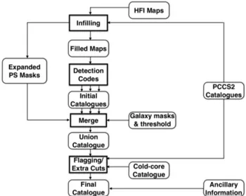
The SZ catalogue construction pipeline is shown in schematic form in Fig.1and largely follows the process used to build the PSZ1. The Planck data required for the construction of the cata-logue comprises the HFI maps (Planck Collaboration VII 2016; Planck Collaboration VIII 2016), point source catalogues for each of the HFI channels (Planck Collaboration XXVI 2016), ef-fective frequencies and beam widths per HFI channel (as shown in Table1), survey masks based on dust emission as seen in the highest Planck channels, and the catalogue of extended Galactic cold-clump detections (Planck Collaboration XXVIII 2016).
The HFI maps are pre-processed to fill areas of missing data (typically a few pixels), or areas with unusable data, specifically bright point sources. Point sources with S /N > 10 in any channel are masked out to a radius of 3σbeam, using a harmonic infilling
algorithm. This prevents spurious detections caused by Fourier ringing in the filtered maps used by the detection algorithms. As a further guard against such spurious detections, we reject any detections within 5σbeamof a filled point source. We have
veri-fied that this treatment reduces spurious detections due to bright point sources to negligible levels in simulations, while reducing the effective survey area by just 1.4% of the sky. Together with
Fig. 1.Pipeline for catalogue construction.
the 15% Galactic dust and Magellanic cloud mask, this defines a survey area of 83.6% of the sky.
After infilling, the three detection codes produce individual candidate catalogues down to a threshold S /N > 4.5. The cat-alogues are then merged to form a union catalogue, using the dust and extended point source masks discussed above to define the survey area. The merging procedure identifies the highest S/N detection as the reference position during the merge and any detections by other codes within 5 arcmin are identified with the reference position. The reference position and S/N are reported in the union catalogue.
PwS can produce a small number of high-significance spuri-ous detections associated with Galactic dust emission. We apply an extra cut of PwS-only detections at S /N > 10 where the spec-trum has a poor goodness-of-fit to the SZ effect, χ2
red> 16.
We also remove five PSZ2 detections that match PSZ1 de-tections confirmed to be spurious by the PSZ1 follow-up pro-gramme (these were the ones that we re-detected; there were many more confirmed spurious detections from the programme). Finally the sample is flagged to identify the various sub-samples discussed in Sect.3.3. The most important of these flags is discussed in the next section.
3.2. Infra-red spurious detections
Cold compact infra-red emission, particularly that due to Galactic cold-clumps, can lead to high-significance spurious de-tections. We identify these detections by searching for 7 arcmin matches with the Planck cold-clump catalogue (C3PO), or with PCCS2 detections at both 545 GHz and 857 GHz. This match-ing radius was chosen because it is the typical size of a Planck detected cold-clump (Planck Collaboration XXVIII 2016).
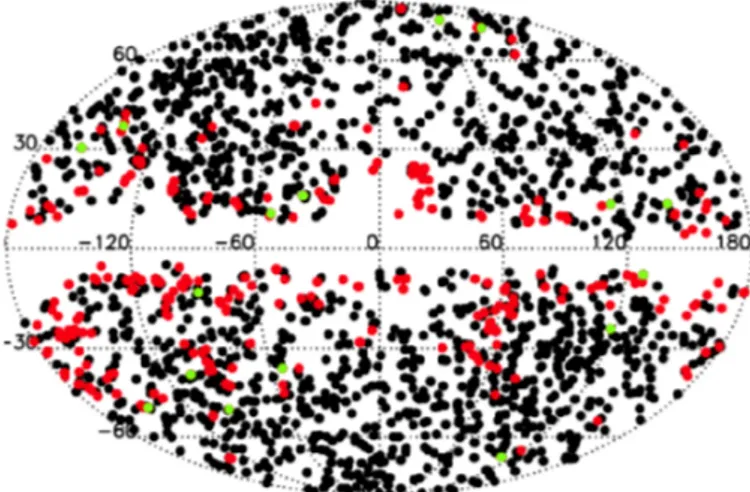
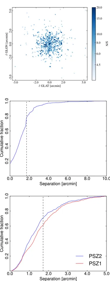
318 raw union detections match these criteria. They tightly follow the distribution of Galactic emission (see Fig.2), such that if the 65% Galactic dust mask (which was used for constructing cluster sample for cosmology used by Planck Collaboration XXIV 2016) is used to define the sample instead of the 85% dust mask, the number of IR-matched raw detections drops to 40. For the high-purity sample formed from the inter-section of all three codes, the numbers are 82 and 13 for the 85% and 65% dust masks respectively. Some high latitude spurious candidates remain. To minimize the effect of spurious detections on the catalogue, we remove these IR matches.
Fig. 2.Distribution of raw SZ detections, with deleted infra-red flagged candidates in red and retained infra-red flagged detections in green. Black points denote detections without an IR flag.
However, we have retained in the sample all 15 confirmed clusters that match these criteria. These IR-contaminated clus-ters represent about 1.5% of the total confirmed clusclus-ters in the PSZ2. In the catalogue, we define a flag, IR_FLAG, to denote the retained clusters that match these criteria; they can be ex-pected to have heavily contaminated SZ signal. This compares well to the 12 contaminated clusters that would be expected from chance alignment if the cluster and IR source populations were uncorrelated.
A small fraction of the unconfirmed detections deleted due to IR-contaminations may have been real clusters. Assuming that optical and X-ray confirmation is unbiased with regard to the presence of IR emission, we estimate these deletions to bias our completeness estimates by less than 1%.
3.3. Catalogue sub-samples
The union catalogue can be decomposed into separate sub-samples, defined as the primary catalogues of the three individ-ual detection codes (PwS, MMF1, MMF3), as well as into unions and intersections thereof. The intersection subsample of candidates detected by all three algorithms can be used as a high-reliability catalogue with less than 2% spurious contamination outside of the Galactic plane (see Sect.4.6).
3.3.1. The cosmology catalogues
We constructed two cluster catalogues for cosmology studies from the MMF3 and the intersection sub-samples, respectively. For these catalogues, our goal was to maximize as much as possi-ble the number of detections, while keeping contamination neg-ligible. A good compromise is to set the S/N threshold to 6 and apply a 65% Galactic and point source mask, as in our 2013 cosmological analysis (Planck Collaboration XX 2014). In this earlier paper, our baseline MMF3 cosmological sample was con-structed using a threshold of 7 on the 15.5 month maps, which is equivalent to 8.5 on the full mission maps. Estimations from the Monte Carlo quality assessment, QA (discussed in Sect.4) suggest that our 2014 intersection sample should be >99% pure for a threshold of 6.
The MMF3 cosmological sample contains 439 detections with 433 confirmed redshifts. The intersection cosmological sample
are clusters, the empirical purity of our samples are >99.8% for MMF3 and >99.6% for the intersection. Note that the intersec-tion sample contains more clusters than the MMF3 sample for the same S/N threshold. This is expected, since the definition of the S/N for the intersection sample is to use the highest value from the three detection methods.
The completeness is also a crucial piece of information. It is computed more easily with the single method catalogue for which the analytical error-function (erf) approximation can be used (as defined in Planck Collaboration XXIX 2014). In Sect. 4.3and inPlanck Collaboration XXIV (2016), we show that this analytical model is still valid for the considered thresh-old. For the intersection sample, we rely on the Monte Carlo estimation of the completeness described in Sect.4.2.
These two samples are used in the cosmological parameter analysis of Planck Collaboration XXIV(2016). Detections that are included in either of the cosmology samples are noted in the main catalogue (see AppendixD).
3.4. Consistency between codes
We construct the union sample using the code with the most sig-nificant detection to supply the reference position and S/N. This contrasts with the PSZ1approach, which used a pre-defined code ordering to select the reference position and S/N. In this section, we demonstrate the consistency of the detection characteristics of the codes for common detections, motivating this change in catalogue construction.
We fit the S/N relation between codes using the Bayesian approach described by Hogg et al. (2010) for linear fits with covariant errors in both variables. We consider the catalogue S/N values to be estimates of a true underlying variable, s, with Gaussian uncertainties with standard deviation σ= 1.
We relate the s values for two different catalogues using a simple linear model
s2= αs1+ A, (6)
where we assume flat priors for the intercept A, and a flat prior on the arc-tangent of the gradient α, such that p(α) ∝ 1/(1+α2). We
also allow for a Gaussian intrinsic scatter between the s values that includes any variation beyond the measurement uncertainty on s. This is parameterised by σint, with an uninformative prior
p(σint) ∝ 1/σint.
We assume a fiducial correlation of ρcorr = 0.8 between the
S/N estimates of each code pair, which is typical of the corre-lation between the matched multi-filtered patches of each code. The fit results are shown in Table2.
The S/N estimates from the three codes are compared in Fig. 3, which also shows the best-fit relation. MMF1 produces noticeably weaker S/N values than the other two codes for the 14 very strong detections at S /N > 20. Excluding these excep-tional cases from the comparison, the best-fit relations between the S/N values from each code show no significant deviations from equality between any of the codes.
There are a small number of highly significant outliers in the relation between PwS and the MMF codes. These are clus-ters imbedded in dusty regions where the different recipes for the filtered patch cross-power spectrum vary significantly and the likelihood assumptions common to all codes break down. PwS shows outlier behaviour relative to the other codes, since its recipe is most different from the other codes.
Fig. 3.Comparison of the S/N estimates from the three detection codes. The dashed green curves show the best-fit relation for a correlation of 0.8 and the red line is the line of equality.
Table 2. Results of fits between S/N from the three detection codes, using the fitting function in Eq. (6).
s1 s2 N A α σint
MMF1 MMF3 1032 −0.01 ± 0.01 1.01 ± 0.01 0.033 ± 0.001
MMF1 PwS 985 −0.02 ± 0.01 1.03 ± 0.02 0.030 ± 0.001
MMF3 PwS 1045 0.00 ± 0.01 1.01 ± 0.01 0.031 ± 0.001
Notes. The assumed correlation of the uncertainties of s1and s2was 0.8.
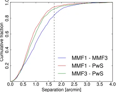
Fig. 4.Cumulative distribution of angular separation between matched
detections for each possible code pair. The vertical dashed line indicates the width of a Healpix pixel at the Planck resolution.
Figure4shows the consistency of the position estimates be-tween the codes. The positions of MMF1 and MMF3 are less consis-tent with one another than any other code combination. The 67% bound on the MMF1−MMF3 separation is 1.3 arcmin, while for MMF1−PwS it is 0.98 arcmin and for MMF3−PwS it is 1.1 arcmin. This is consistent with the observation from the quality assess-ment that the PwS positions are the most robust (Sect.4.4).
4. Selection function
A necessary element of any cluster sample is the selection func-tion that relates the detected sample to the underlying populafunc-tion
of objects. The selection function comprises two complementary functions: the completeness, which defines the probability that a given real object will be detected; and the statistical reliability, also known as purity, which defines the probability that a given detection corresponds to a real object. As a function of ing object attributes, the completeness is a function of underly-ing SZ observables, θ500and Y500. The reliability is a statistical
function of detection attributes and is presented as a function of detection S/N.
4.1. Monte-Carlo Injection
The selection function is determined by the Monte-Carlo injec-tion of simulated clusters into both real and simulated Planck maps. A common segment is the injection of cluster SZ signal. The cluster signal is assumed to be spherically symmetric and to follow a pressure profile similar to the generalized Navarro-Frenk-White (GNFW) profile assumed in the catalogue extrac-tion (Nagai et al. 2007;Arnaud et al. 2010).
To include the effects of system-on-system variation in the pressure distribution, we draw the spherically-averaged individ-ual pressure profiles from a set of 910 pressure profiles from simulated clusters coming from the cosmo-OWLS simulations (Le Brun et al. 2014; McCarthy et al. 2014), an extension of the OverWhelmingly Large Simulations project (Schaye et al. 2010). These pressure profiles are empirical in the sense that they have not been fitted using a GNFW profile: the mean pressure is used within concentric radial shells (after the subtraction of ob-vious sub-structures) and the injected profiles are interpolated across these shells. The simulated clusters were selected for this sample by requiring that their mass be above the approximate limiting mass for Planck at that redshift. The ensemble of sim-ulated profiles are shown in Fig. 5. Each profile is normalized such that the spherically integrated Y500parameter matches the
Fig. 5.The 910 simulated pressure profiles from the cosmo-OWLS sim-ulations used for cluster injection. Also shown are the assumed extrac-tion profile (UPP) and the best-fit profile from a sample of 62 pressure profiles fitted using Planck and X-ray data (PIPV,Planck Collaboration
Int. V 2013).
(Y500, θ500) are different for completeness and reliability
simula-tions and each is discussed below.
Effective beam variation is an important consideration for the unresolved clusters at the intermediate and high redshifts of cos-mological interest. We deal with this by convolving the injected clusters with effective beams in each pixel including asymmetry computed followingMitra et al.(2011)
4.2. Completeness
The completeness is defined as the probability that a cluster with a given set of true values for the observables (Y500, θ500) will
be detected, given a set of selection criteria. A good approxi-mation to the completeness can be defined using the assumption of Gaussianity in the detection noise. In this case, the complete-ness for a particular detection code, χ, follows the error function (erf()), parametrized by a selection threshold q and the local detection noise at the clusters radial size, σY(θ500, φ, ψ),
χ(Y500, θ500, φ, ψ) = 1 2 " 1 − erf Y500√− qσY(θ500, φ, ψ) 2σY(θ500, φ, ψ) !# · (7)
This approach is not suited to the union and intersection cata-logues from Planck, due to the difficulty in modelling correla-tions between detection codes. We determine the completeness by brute force, injecting and detecting simulated clusters into the Plancksky maps. This approach has the advantage that all algo-rithmic effects are encoded into the completeness, and the effects of systematic errors, such as beam and pressure profile vari-ation, can be characterized. This approach also fully accounts for the non-Gaussianity of the detection noise due to foreground emission.
The injected (Y500, θ500) parameters are drawn from a
uni-form distribution in the logarithm of each variable, ensuring that our logarithmically spaced completeness bins have approx-imately equal numbers of injected sources.
As the completeness is estimated from injection into real data, injected sources can contribute to the detection noise. We therefore use an injection mode, as was the case for the PSZ1 completeness, where injected clusters are removed from
real data detections. Together, these ensure that the noise statis-tics for injected clusters are the same as for the real detections in the map.
We release as a product the Monte-Carlo completeness of the catalogues at thresholds stepped by 0.5 in S/N over the range 4.5 ≤ S /N ≤ 10. Figure6shows the completeness of the union and intersection catalogues as functions of input (Y500, θ500) and
at representative values of θ500, for three detection thresholds.
The union and intersection catalogues are most similar at high S/N, where they match well except at small scales. Here the in-tersection catalogue follows the lower completeness of MMF1. This is due to an extra selection step in that code, which re-moves spurious detections caused by point sources. The union and intersection catalogues mark the upper and lower limits of the completeness values for the sub-catalogues based on the in-dividual codes.
The completeness of the Planck cluster catalogue is robust with respect to deviations of the real SZ profiles of galaxy clus-ters from the one assumed by the algorithms for filter construc-tion. To demonstrate this, we compare χMC, the Monte-Carlo
completeness for the MMF3 sample, using the cosmoOWLs pro-file variation prescription and effective beam variation, to χerf,
the semi-analytic erf() completeness given by Eq. (7). This comparison is shown in Fig.7, where we show the difference be-tween the two estimates as a function of Y500and θ500. We also
show the individual completeness values as functions of Y500for
representative values of θ500.
The error function is a good approximation to the MC com-pleteness for the cosmology sample, which uses a higher S/N cut and a larger Galactic mask than the full survey. The MC estimate corrects this analytic completeness by up to 20% for large re-solved clusters, where χMCis systematically lower than the erf()
expectation, primarily due to variation in the cluster pressure profiles. For unresolved clusters, the drop-off in χMCis slightly
wider than the erf() expectation, reflecting variation both of pressure profiles and of effective beams.
The impact of these changes in completeness on expected number counts and inferred cosmological parameters for the cosmology sample is analysed in Planck Collaboration XXIV (2016). The difference between the Monte Carlo and erf() com-pleteness results in a change in modelled number counts of typ-ically 2.5% (with a maximum of 9%) in each redshift bin. This translates into a 0.26σ shift of the posterior peak for the implied linear fluctuation amplitude, σ8.
The MC completeness is systematically lower than the an-alytic approximation for the full survey. One of the causes of this is Galactic dust contamination, which is stronger in the ex-tra 20% of the sky included in the full survey area relative to the cosmology sample area. This tends to reduce the S/N of clusters on affected lines of sight.
We note that this approach ignores other potential astrophys-ical effects that could affect the completeness. Radio emission is known to be correlated with cluster positions, potentially “filling in” the SZ decrement, though recent estimates suggest that this effect is typically small in Planck data (Rodriguez-Gonzalvez et al. 2015). Departures of the pressure distribution from spher-ical symmetry may also affect the completeness, though this ef-fect is only likely to be significant for nearby and dynamically disturbed clusters, which are not small compared to the Planck beams. We test for some of these effects through external val-idation of the completeness in the next section, and explicitly through simulation in Sect.4.5.
Fig. 6.Completeness of the union and intersection samples at progressively lower S/N thresholds. From left to right, the thresholds are 8.5, 6.0 and 4.5 (the survey threshold). In the top panels, the dotted lines denote 15% completeness, the dashed lines 50%, and the solid lines 85% completeness. In the bottom panels, the union is denoted by the diamonds with Monte Carlo uncertainties based on binomial statistics, and the intersection is denoted by the solid lines.
Fig. 7.Differences between the semi-analytic and Monte Carlo completenesses for MMF3. The left panels show the difference for the full survey
over 85% of the sky with a q= 4.5 threshold. The right panels show the difference for the MMF3 cosmology sample, covering 65% of the sky to a threshold of q= 6.0. The top panels show the difference χMC−χerfas a percentage. The bottom panels compare the completenesses at particular θ500values. The Monte-Carlo completeness is denoted by diamonds and the erf() completeness by solid lines.
Fig. 8. MMF3 completeness for the PSZ2 catalogue (S/N threshold q > 4.5) determined from the MCXC (left) and SPT (right) catalogues. This external estimate (red histogram) is in good agreement with the analytic erf() calculation (solid blue line), except for SPT at the high probability end (see text).
Another source of bias is the presence of correlated IR emis-sion from cluster member galaxies.Planck Collaboration XXIII (2016) shows that IR point sources are more numerous in the di-rection of galaxy clusters, especially at higher redshift, and con-tribute significantly to the cluster SED at the Planck frequencies. Initial tests, injecting cluster signals with the combined IR+tSZ spectrum of z > 0.22 clusters observed inPlanck Collaboration XXIII(2016), suggest that this reduces the completeness for un-resolved clusters. The effective detection threshold can move upwards by up to 30% for unresolved clusters (θ500 < 7
ar-cmin), though no significant changes appear for resolved clus-ters . Future work is warranted to characterize the evolution and scatter of this IR emission and to propagate the effect on com-pleteness through to cosmological parameters.
4.3. External validation of the completeness
We validated our Monte Carlo completeness calculation and the simple analytical erf() model in Eq. (7) by using the MCXC (Piffaretti et al. 2011) and SPT (Bleem et al. 2015) cat-alogues. The Planck detection threshold is passed across the cluster distributions of these two samples. This is illustrated in Fig. 4 of Chamballu et al.(2012) for the MCXC. This allows us to characterize our completeness by checking if the frac-tion of detected clusters follows the expected probability dis-tribution as a function of their parameters. For each cluster of the MCXC catalogue, we use the MMF3 algorithm to extract its flux Y500 and associated error σY at the location and for
the size given in the X-ray catalogue. We then build the quan-tity δ = (Y500− qσY)/
√
2σY, q being the detection threshold
(here 4.5) and σY the noise of the filtered maps. We make the
corresponding histogram of this quantity for all the clusters and for the clusters detected by MMF3. The ratio of the two histograms is an empirical estimate of the completeness. Results are shown in Fig.8for the MCXC (left) and the SPT (right) catalogues. For MCXC, the estimation is in good agreement with the expected simple analytical erf() model (0.5 (1+ erf(δ))). For SPT, the es-timated completeness is also in good agreement except for δ > 1 where it is higher than the analytic expectation. We attribute this behaviour to the correlation between SPT and Planck detections. The SPT catalogue is SZ-based, so a cluster detected by SPT will have a higher than random probability to be detected by Planck.
This leads to an overestimation of the completeness at the high probability end.
4.4. Position estimates
We characterize the positional recovery of the Planck detections using source injection into real data, including pressure profile and beam variation. We draw input clusters from a realistic dis-tribution of (Y500, θ500), which is the same as used for the
relia-bility in Sect.4.6.
Figure9shows the comparative performance of the individ-ual detection codes, and of the reference position chosen for the union catalogue. PwS produces the most accurate positions, with 67% of detected positions being within 1.18 arcmin of the input position. For MMF1 and MMF3, the 67% bound is 1.58 arcmin and 1.52 arcmin, respectively. The union and intersection accuracy follow that of the MMFs, with 67% bounds of 1.53 arcmin. We observe that our inter-code merging radius of 5 arcmin is conser-vative, given the expected position uncertainties.
4.5. Impact of cluster morphology
Clusters are known to possess asymmetric morphologies and a wide range of dynamical states, from irregular merging clusters to regular relaxed clusters. While the completeness simulations have included some morphology variations through variation of the injected radial pressure profile, this ignores the effects of the sub-structures and asymmetries, which may induce detection bi-ases for large clusters at low redshift resolved by the Planck beams, FWHM ≈ 7 arcmin.
Neither of the external samples used in Sect.4.3to validate the completeness allow us to properly probe resolved, irregular clusters at low-redshift. The MCXC is biased towards regular clusters, due to X-ray selection effects, while the Planck com-pleteness drop-off lies substantially beneath the SPT mass limit at low redshift, so this drop-off is not sampled.
We address the effects of realistic morphology by injecting into the Planck maps the raw 2D projected Compton-Y sig-nal from a sample of hydrodynamically simulated cosmoOWLs clusters. The clusters were injected with a large enough angu-lar extent, θ500 = 20 arcmin, that they were resolvable in the
Fig. 9. Cumulative distribution of angular separations between esti-mated and input positions. The dashed vertical line denotes the Planck pixel size.
expected completeness drop-off. 20 candidate clusters were cho-sen from the sub-sample of cosmoOWLS clusters selected by the mass cuts discussed in Sect.4.1, based on their dynamical state. The ten clusters in the sub-sample with the highest kinetic-to-thermal energy ratio within θ500 constituted our “disturbed”
sample, while the “regular” sample comprised the ten clusters with the lowest kinetic-to-thermal energy ratio within θ500. These
clusters were injected 200 times, randomly distributed across the sky. We also created simulations injecting symmetric clusters with the UPP with the same parameters and locations as the hydrodynamic projections. In all cases, the signals were con-volved with Gaussian beams.
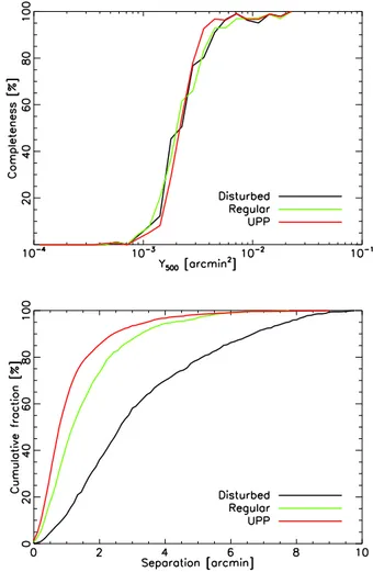
The completeness for regular, disturbed and UPP clusters is shown for the union catalogue in the top panel of Fig. 10. There are no significant differences between the completeness functions for the regular and disturbed clusters. Both sets of hy-drodynamic clusters show a slight widening effect in the com-pleteness, caused by the variation in the effective pressure pro-file away from the UPP assumed for extraction (the same effect as discussed in Sect.4.2).
Morphology has a clear impact on the estimation of clus-ter position. The bottom panel of Fig.10shows the cumulative distribution of angular separation between union and input posi-tions for the regular, disturbed and UPP clusters. The disturbed clusters show a significant reduction in positional accuracy. Part of this is physical in origin. The cluster centres were defined here as the position of the “most-bound particle”, which traces the minimum of the gravitational potential and is almost always coincident with the brightest central galaxy. For merging clus-ters this position can be significantly offset from the centre of the peak of the SZ distribution. A matching radius of 10 arcmin, which is used in Sect.7, ensures correct identification of detected and injected positions.
4.6. Reliability
The statistical reliability is the probability that a detection with given detection characteristics is a real cluster. We determine the reliability using simulations of the Planck data. Clusters are injected following the prescription in Sect.4.1, except that the
Fig. 10.Impact of cluster morphology on the completeness (top panel)
and position estimates (bottom panel) for resolved clusters. The simu-lated clusters are all injected with θ500= 200, and all curves are for the union catalogue. Cluster morphology has no impact on the complete-ness, but a significant impact on the position estimation.
clusters are injected such that cluster masses and redshifts are drawn from aTinker et al.(2008) mass function and converted into the observable parameters (Y500, θ500) using the Planck ESZ
Y500–M500scaling relation (Planck Collaboration X 2011). The
other components of the simulations are taken from FFP8 sim-ulation ensemble (Planck Collaboration XII 2016). The compo-nents include a model of Galactic diffuse emission, with ther-mal dust (including some emission from cold-clumps), spinning dust, synchrotron and CO emission, and extra-galactic emis-sion from the far IR background. The diffuse components are co-added to a set of Monte Carlo realizations of CMB and strumental noise. In addition to the cluster signal, we also in-ject point sources drawn from a multi-frequency model from the Plancksky model (Planck Collaboration XII 2016). These point sources are mock detected, using completeness information from the PCCS2 (Planck Collaboration XXVI 2016), and harmoni-cally infilled using the same process as for the real maps prior to SZ detection. This leaves a realistic population of residual sources in the maps. After detection, candidates that lie within the simulated expanded source mask, or which match with the cold-core or IR source catalogues from the real data, have their S/N values set to zero.
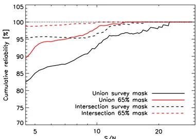
Figure11shows the reliability as a function of S/N for the union and intersection samples across the whole survey area and
Fig. 11.Cumulative reliability as a function of S/N.
outside the 65% Galactic mask used to define the cosmology samples. Relative to the PSZ1, the reliability of the union sample has improved by 5%, the lower noise levels have revealed more “real” simulated clusters than spurious detections. As was the case with the PSZ1, the reliability is improved significantly by removing more of the Galactic plane, where diffuse and compact Galactic emission induces extra spurious detections.
4.7. Neural network quality assessment
We supplement the simulation-based reliability assessment with an a posteriori assessment using an artificial neural-network. The construction, training, and validation of the neural network is discussed fully in Aghanim et al.(2015). The network was trained on nominal mission Planck maps, with a training set composed of three elements: the positions of confirmed clusters in the PSZ1 as examples of good cluster signal; the positions of PCCS IR and radio sources as examples of point-source induced detections; and random positions on the sky as examples of noise-induced detections. We provide for each detection a neural network quality flag, Q_NEURAL= 1−Qbad, following the
def-initions inAghanim et al.(2015), who also tested the network on the unconfirmed detections in the PSZ1. They showed that this flag definition separates the high quality detections from the low quality detections, as validated by the PSZ1 external validation process, such that Q_NEURAL < 0.4 identifies low-reliability detections with a high degree of success.
459 of the 1961 raw detections possess Q_NEURAL < 0.4 and may be considered low-reliability. This sample is highly correlated with the IR_FLAG, 294 detections being in com-mon. After removal of IR spurious candidates identified by the IR_FLAG, as discussed in Sect. 3.2, we retain 171 detections with bad Q_NEURAL, of which 28 are confirmed clusters. This leaves 143 unconfirmed detections considered likely to be spuri-ous by the neural network.
The Q_NEURAL flag is sensitive to IR induced spurious detections. The detections with low Q_NEURAL quality flag are clustered at low Galactic latitudes and at low to intermedi-ate S/N. This clustering is not seen for realization-unique spuri-ous detections in the reliability simulations, which are identifi-able as noise-induced. The reliability simulations underestimate the IR spurious populations relative to the Q_NEURAL flag. Conversely, the neural network flag by construction does not target noise-induced spurious detections: Qbad is the parameter
Fig. 12.Lower limits on the catalogue reliability, estimated by
combin-ing the reliability simulations with the Q_NEURAL information (see text).
trained to indicate IR-induced spurious sources. The neural net-work flag also has some sensitivity to the noise realization and amplitude in the data; the assessment is different to that applied to the nominal mission maps in Planck Collaboration XXXII 2015.
To place a lower limit on the catalogue reliability, we com-bine the Q_NEURAL information with the noise-induced spuri-ous detections from the reliability simulations. For each reliabil-ity simulation realization, we remove the simulated IR-spurious detections, which can be identified either as induced by the FFP8 dust component, and thus present in multiple realizations, or as induced by injected IR point sources. We replace these spurious counts with the unconfirmed low Q_NEURAL counts, smoothed so as to remove the steps due to small number statistics.
The combined lower limit of the reliability is shown in Fig. 12. The lower limit tracks the simulation reliability well outside the 65% Galactic dust mask. For the whole survey re-gion, the lower limit is typically 6% lower than the simulation estimate, due either to over-sensitivity of the neural network to dusty foregrounds, or shortcomings in the FFP8 Galactic dust component.
5. Parameter estimates
The SZ survey observable is the integrated Comptonization pa-rameter, YSZ. As was the case for the PSZ1, each of the
extrac-tion codes has an associated parameter estimaextrac-tion code that eval-uates, for each detection, the two dimensional posterior for the integrated Comptonization within the radius 5R500, Y5R500, and
the scale radius of the GNFW pressure θS. The radius 5R500 is
chosen because it provides nearly unbiased (to within a few per-cent) estimates of the total integrated Comptonization parame-ter, while being small enough that confusion effects from nearby structures are negligible.
We provide these posteriors for each object and for each code, and also provide Y5R500in the union catalogue, defined as
the expected value of the Y5R500marginal distribution for the
ref-erence detection (the posterior from the code that supplied the union position and S/N).
Below we also discuss the intricacies of converting the pos-teriors to the widely used X-ray parameters Y500and θ500.
Fig. 13.Top: results of the posterior validation for Y5R500. The histogram of the posterior probability, ζ, bounded by the true Y5R500 parameter, is almost uniformly distributed, except for a small excess in the tails of the posteriors, at ζ > 0.95. The histogram has been normalised by the expected counts in each ζ bin. Bottom: comparison of recovered peak Y5R500to the injected Y5R500. The estimates are unbiased, though asymmetrically scattered, with a scatter that decreases as S/N increases.
5.1. Y5R500estimates
To validate the Y5R500 estimates, we apply the posterior
val-idation process introduced in Harrison et al. (2015) to the
Y5R500marginal distributions. In brief, this process involves
sim-ulating clusters embedded in the Planck maps and evaluating the (Y, θ) posteriors for each (detected) injected cluster. For each posterior, we determine the posterior probability, ζ, bounded by the contour on which the real underlying cluster parameters lie. If the posteriors are unbiased, the distribution of this bounded probability should be uniformly distributed between zero and one.
This process allows us to include several effects that vi-olate the assumptions of the statistical model used to esti-mate the posteriors. Firstly, by injecting sources into real sky maps, we include non-Gaussian contributions to the noise on the multi-frequency matched-filtered maps that come from Galactic diffuse foregrounds and residual point sources. Secondly, we include violations of the “signal” model that come from dis-crepancies between the cluster pressure profile and the UPP as-sumed for parameter estimation, and from position dependent
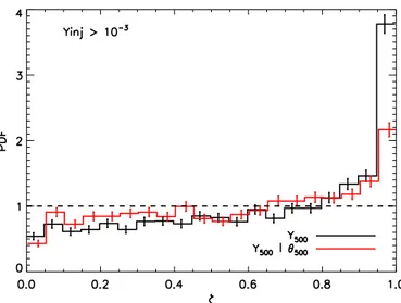
Fig. 14.Bounded probability histograms, as in the top panel of Fig.13,
but for the converted p(Y500) marginal and p(Y500|θ500) sliced posteriors. The values of Y500that we injected were all >10−3arcmin2.
and asymmetric effective beams that vary from the constant Gaussian beams assumed for estimation. The clusters are in-jected using the process discussed in Sect. 4.1, drawing in-jected pressure profiles from the set of cosmo-OWLs simulated profiles.
The top panel of Fig. 13shows the histogram of ζ for the PwS Y5R500marginals. The distribution is flat, except for a small
excess in the 0.95–1.0 bin, which indicates a small excess of out-liers beyond the 95% confidence region (in this case 52% more than statistically expected). This suggests that the posteriors are nearly unbiased, despite the real-world complications added to the simulations. Note that we have considered only posteriors where the injected Y5R500 > 0.001 arcmin2, a cut that removes
the population effects of Eddington bias from consideration; we focus here on the robustness of the underlying cluster model.
The bottom panel of Fig.13shows the peak recovery from the PwS Y5R500 marginals compared to the true injected values.
The peak estimates are unbiased relative to the injected parame-ters: a regression analysis of the peak estimates gives a slope of unity and a bias of 2.6%.
5.2. Conversion to Y500
The (Y5R500,θS) estimates can be converted into (Y500, θ500)
esti-mates using conversion coefficients derived from the UPP model that was assumed for extraction. However, when the underly-ing pressure distribution deviates from this model, the conver-sion is no longer guaranteed to accurately recover the underly-ing (Y500, θ500) parameters; variation of the pressure profile can
induce extra scatter and bias in the extrapolation.
We demonstrate this by applying the posterior validation process to the Y500 posteriors, defined as the Y5R500 posteriors
scaled with the UPP conversion coefficient, as estimated from injected clusters whose pressure profiles are drawn from the cos-moOWLS pressure profile ensemble. We validate posteriors for Y500calculated in two ways: firstly by marginalizing over the θ500
parameter, referred to in previous publications as “Y blind”; and secondly by slicing the (Y500, θ500) posteriors at the true value
of θ500, equivalent to applying an accurate, externally measured
delta-function radius prior.
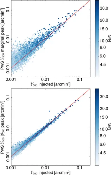
Figure14shows the bounded probability histograms for the two Y500 posteriors and Fig. 15 shows the scatter of the peak
Fig. 15.Scatter of the recovered estimates of Y500with the input Y500. Top: for the marginalised Y500 posterior, “Y blind”. Bottom: for the sliced posterior p(Y500|θ500), assuming an accurate radius prior.
of the posteriors with the input values of Y500. The marginal
Y500 posteriors are poor, with histograms skewed towards the
tails of the distribution and large numbers of >2σ outliers. The scatter plot reveals the peak estimates to possess a large scat-ter and to be systematically biased high by 16%. In contrast, the peak p(Y500|θ500) estimates have much better accuracy and
precision and are distributed around the input values with low scatter and a bias of −2%. The bounded probability histogram of p(Y500|θ500) shows that while there is a noticeable excess of
detections in the wings, the posteriors are reasonably robust. If the posteriors were Gaussian, the skewness of the p(Y500|θ500)
histogram towards the tails would be consistent with an under-estimate of the Gaussian standard deviation of 21%.
We therefore recommend that, to estimate Y500 accurately
from Planck posteriors, prior information be used to break the (Y500, θ500) degeneracy. However, we note that the uncertainties
on such Y500estimates will be slightly underestimated.
5.3. Mass and Y500 estimates using scaling priors
The key quantity which can be derived from SZ observables is the total mass of the detected clusters within a given overden-sity (we used∆ = 500). To calculate the mass from Planck data
0.005 0.010 0.015 10 20 30 40 θ s [arcmin] Y 5R500 [arcmin 2 ]
Fig. 16.Illustration of the posterior probability contours in the Y5R500–θs
plane for a cluster detected by Planck. The contours show the 68, 95 and 99% confidence levels. The red continuous line shows the ridge line of the contours, while the dashed lines are the ±1σ probability value at each θS. The cyan line is the expected relation from Arnaud et al. (in prep.) at a given redshift.
it is necessary to break the size-flux degeneracy by providing prior information, as outlined in the previous section. We used an approach based on Arnaud et al. (in prep.), where the prior information is an expected function relating Y500 to θ500 that
we intersect with the posterior contours. We obtained this re-lation by combining the definition of M500(see Eq. (9) inPlanck
Collaboration XX 2014, connecting M500 to θ500, for a given
redshift z) with the scaling relation Y500–M500 found inPlanck
Collaboration XX(2014). A similar approach was also used in Planck Collaboration XXIX(2014), but now we use the full pos-terior contours to associate errors to the mass value.
We illustrate our method in Fig. 16. At any fixed value of θS, we study the probability distribution and derive the Y5R500
associated to the maximum probability, i.e. the ridge line of the contours (red continous line in Fig.16). We also derive the Y5R500
limits enclosing a 68% probability and use them to define an upper and lower degeneracy curve (dashed lines). From the in-tersection of these three curves with the expected function, we derive the MSZ estimate and its 1σ errors, by converting Y5R500
to Y500and then applying the Y500–M500scaling relation prior at
the redshift of the counterpart.
MSZ can be viewed as the hydrostatic mass expected for a
cluster consistent with the assumed scaling relation, at a given redshift and given the Planck(Y–θ) posterior information. We find that this measure agrees with external X-ray and optical data with low scatter (see Sect.7). For each MSZ measurement, the
corresponding Y500from the scaling relation prior can be
calcu-lated by applying the relation.
We underline that the errors bars calculated from this method consider only the statistical uncertainties in the contours, not the uncertainties on the pressure profile nor the errors and scatter in the Y500–M500scaling relation, and should thus be considered a
lower limit to the real uncertainties on the mass.
We use the masses for the confirmation of candidate counter-parts (see Sect.7) and we provide them, along with their errors, in the PSZ2 catalogue, for all detections with confirmed redshift. We compared them with the masses provided in PSZ1 for the de-tections where the associated counterpart (and thus the redshift value) has not changed in the new release (see Appendix B).
Table 3. Results of fits between S/N from the PSZ1 and PSZ2, using the fitting function in Eq. (6).
s1 s2 A α σ
PSZ2 PSZ1 0.76 ± 0.08 0.72 ± 0.01 0.53 ± 0.02
Notes. The assumed correlation of the uncertainties of s1 and s2 was 0.72.
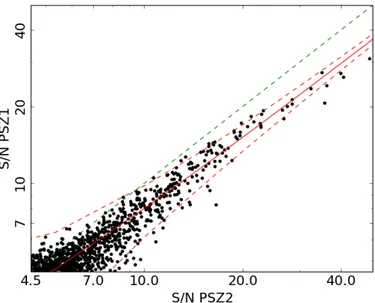
Fig. 17.Comparison of S/N values for common PSZ1 and PSZ2
detec-tions. The best fit relation is plotted in red, with 2σ scatter shown by dashed red lines. The green dashed line denotes the 1-to-1 relation.
We find very good agreement between the two values, which are consistent within the error bars over the whole mass range.
In the individual catalogues, we provide for all entries an array of masses as a function of redshift, MSZ(z), which we
ob-tained by intersecting the degeneracy curves with the expected function for different redshift values, from z = 0 to z = 1. The aim of this function is to provide a useful tool for counterpart searches: once a candidate counterpart is identified, it is su ffi-cient to interpolate the MSZ(z) curve at the counterpart redshift
to estimate its mass.
6. Consistency with the PSZ1
The extra data available in the construction of the PSZ2 improves the detection S/N and reduces statistical errors in the parameter and location estimates. Here we assess the consistency between the two catalogues, given the matching scheme discussed in Sect.7.1.
6.1. Signal-to-noise
We fit the relation between S/N for common PSZ1 and PSZ2 clusters using the approach and model discussed in Sect.3.4. For the PSZ1 and PSZ2, the likelihoods for s1 and s2 have a strong
covariance, since more than half of the PSZ2 observations were used in the construction of the PSZ1. We therefore assign a co-variance of 0.72 between the two S/N estimates, as is appropri-ate for Gaussian errors sharing 53% of the data. As the errors are not truly Gaussian, we allow for an intrinsic scatter between the S/N estimates to encapsulate any unmodelled component of the S/N fluctuation.
The consistency of the S/N estimates between the PSZ1 and PSZ2 are shown in Fig.17and the best fitting model is shown in Table3. Detections with PSZ2 S /N > 20 are affected by changes in the MMF3 S/N definition. For the PSZ1, the empirical standard deviation of the filtered patches was used to define the S/N in this regime, while the theoretical standard deviation of Melin et al.(2006) was used for lower S/N. MMF3 now uses the the-oretical standard deviation for all S/N, consistent with the ESZ and the definitions in the other detection codes. For this reason, the best fit model ignores detections at S /N > 20 in either cat-alogue. The MMF3 S/N show a flat improvement relative to the ESZ S/N (which was produced solely by MMF3), consistent with the reduced noise in the maps.
If the Compton-Y errors are entirely Gaussian in their be-haviour, we should expect the S/N to increase by 37% between the PSZ1 and PSZ2, i.e., α= 0.73. This is consistent within 1σ with the fit, which describes the S/N behaviour well to S/N < 20.
6.2. Position estimation
The distribution of angular separations between the PSZ2 and PSZ1 position estimates is shown in Fig.18. Of the common de-tections, 80% of the PSZ2 positions lie within one Planck map pixel width, 1.7 arcmin, of the PSZ1 position. MMF3 does not al-low for sub-pixel positioning, so if the MMF3 position was used for the union in both the PSZ1 or PSZ2, the angular separation will be a multiple of the pixel width. This is evident in the cu-mulative distribution of angular separations as discontinuities at 0, 1, and √2 pixel widths.
We also compare the position discrepancy between the SZ detection and the X-ray centres from the MCXC (Piffaretti et al. 2011). The bottom panel of Fig.18 shows the distributions of these angular separations for the PSZ2 and PSZ1. The distribu-tions are calculated from the full MCXC match for each cata-logue: the PSZ2 includes 124 new detections. The PSZ2 posi-tion estimates are clearly closer to the X-ray centres than the PSZ1; for the PSZ1, the 67% error radius is 1.85 arcmin, while for the PSZ2 this reduces to 1.6 arcmin. The expected statistical improvement of the position discrepancy due to the new Planck data is a reduction to 1.35 arcmin. This suggests Planck posi-tional uncertainty is not the only contributor to this offset. For example a physical offset between X-ray and SZ centroids is possible, with offsets of up to arcminute scales observed in com-parisons of SZ and X-ray data for dynamically disturbed clusters (Planck Collaboration Int. IV 2013;Reichardt et al. 2013).
6.3. Missing PSZ1 detections
The PSZ1 produced 1227 union detections. While the numbers of detections has increased by 35% in the PSZ2 to 1653, the number of common detections is 936, so 291 (23.7%) of the PSZ1 detections disappear. The high-purity intersection sample loses 44 detections, of which 20 are lost entirely, and 24 drop out of the intersection after one or two codes failed to detect them. In this section, we discuss these missing detections. TableE.1 de-tails each of the missing detections and provides an explanation for why each is missing.
The first type of missing detection are those that fall un-der the new survey mask, due to the increase in the number of point sources being masked. The masked areas are pre-processed with harmonic infilling to prevent spurious detections induced by Fourier ringing. The increase of the mask area is driven