Macroeconomic Instability and the Phillips Curve in Italy
by Alessandra Del Boca, Michele Fratianni, Franco Spinelli and Carmine Trecroci1. Introduction
Inflation dominated the policy agenda for much of the 1970s and the 1980s. Over the next two decades, greater macroeconomic stability (the «Great Moderation») has confined the issue to the outer limits of the macro-economic debate. In the light of recent developments, this was shortsighted. Between 2005 and the current downturn (2008-9), inflation rates and expec-tations rose across most advanced economies, suggesting that inflation is not dead and continues to be worth studying it, mainly for its policy relevance and its impact on long-term macroeconomic performance. Shedding some light on unsettled aspects of past inflationary processes could also guide us in interpreting the current state of affairs and in identifying forces that trigger major inflation shocks. This paper contributes to the debate by investigat-ing the tradeoff between inflation and output in Italy and its evolvinvestigat-ing nature, with a focus on the post-WWII years.
There are at least three motivations for the choice of Italy as a case study. The first is that this country has experienced higher than average and more volatile inflation rates than most other industrialized economies across a va-riety of monetary regimes. The second is that Italy differs markedly from Anglo-Saxon market structures and institutions, on which the bulk of the Phillips curve literature has focused. Among the differences, rigidities in the labor market stand out. At the end of the 1960s, in step with the widespread union unrest in industrialized countries, Italian unions managed to impose a unique two-tier bargaining system – at the national and firm levels – keyed
Received December 2010, Approved November 2011.
We thank participants to the AIEL 2008 (Brescia), ESAM 2008 (Wellington) and SIE 2011 conferences, and Chris Gilbert, Patrizio Bianchi, Giovanni Pittaluga and two anonymous referees for very valuable comments and suggestions. An earlier draft of this paper circulated under the title «Wage bargaining and the Phillips Curve in Italy».
on an indexation mechanism called the Scala Mobile (SM). SM, inspired by a strong egalitarian motivation, held at centre stage until the early 1990s and exacerbated the inflationary process. Symmetrically, subsequent changes in the wage bargaining structure and in the indexation mechanism contributed, in addition to a tighter monetary policy, to the decline of inflation in the re-mainder of the 1990s and eased Italian membership in the European Mon-etary Union (EMU). Finally, the course of post-war Italian monMon-etary policy was critically influenced by government financing requirements, a specific application of fiscal dominance (Fratianni - Spinelli, 2001b).
This paper asks whether the combination of a rigid wage indexation mechanism and a regime of fiscal dominance were responsible for the Ital-ian inflation process to be significantly distinct when compared with other advanced countries. We evaluate this distinctiveness using the key metric of the inflation-output tradeoff. Methodologically, we first examine the volatil-ity, persistence and stationarity properties of the Italian inflation rate across various exchange-rate regimes that have characterized post-WWII Italian monetary history (Fratianni - Spinelli, 2001a). Next, we estimate alternative Phillips equations, and study the effects of structural changes and asymme-tries on the estimated parameters of the inflation-output tradeoff. For that, we rely on a time-varying parameter model estimated with a Kalman filter algorithm.
Our key results are as follows. The statistical properties of inflation dis-play significant fluctuations over the post-WWII sample. Periods of fixed ex-change rates and looser wage bargaining mechanisms, often accompanied by less accommodative monetary policies, were associated with lower and more stable inflation rates than periods characterized by more rigid labor mar-ket regulation and flexible exchange rates. As a result, we uncover signifi-cant evidence of structural breaks in the inflation process, which makes the standard, constant-coefficient approaches to the study of the output-inflation correlation very questionable. A fitting example is the 1972-84 period, which stands out as the only non-war episode of high inflation. After the demise of the Bretton Woods agreement, strict wage indexation made Italian wages sensitive to prices of imported goods, in fact contributing to importing for-eign inflation. Furthermore, the high rate of government budget deficit mon-etization produced expansionary monetary policies and recurrent exchange-rate crises, while inflation shocks and uncertainty hit hardest groups whose incomes were less sheltered by indexation. These effects lasted in Italy much longer than in comparable economies, at least until 1985. In that year, Italy started a slow adjustment process aimed at participating first in the Single European Market and later in the EMU.
We gather evidence on the inflation-output tradeoff using a standard specification that blends the original expectation-augmented Phillips curve with more recent specifications based on persistence and price-wage rigidity. Our main finding is that both traditional OLS methods and more appropri-ate approaches accounting for structural change yield no significant feedback
from cyclical economic conditions to inflation; that is, we cannot detect a statistically significant inflation-output tradeoff. Moreover, we find some evi-dence that the growth in the Treasury component (i.e., linked to government borrowing requirements) of the monetary base is correlated with inflation. This result is consistent with the hypothesis that both labor market rigidities and a fiscally dominated monetary policy were the main drivers of Italian in-flation.
The paper is organized as follows. In Section 2, we present the stylized facts on Italian inflation, on the link between monetary aggregates and bud-get deficits, and on the indexation mechanism. In Section 3, we analyze the statistical properties of the inflation rate and their constancy. In Section 4, we present various estimates of the inflation-output equations, using conven-tional and time-varying methods. Section 5 discusses the main findings of our work and draws some conclusions.
2. Purchasing power in Italy, 1949-2010
2.1. Stylized facts
There are several ways to measure the Italian price level over the long run. Spinelli - Trecroci (2008) and Del Boca et al. (2010) focus on the im-plicit price deflator of national income, cost of living and wholesale prices, dating back to 1861, the year of political unification in Italy. Here, we select the implicit price deflator, but our findings do not change significantly with alternative measures of the price level.
The post-WWII period is the reference sample of our analysis. However, it is helpful to put recent developments into a longer, historical perspective; therefore, we plot in Figure 1 the annual price level from 1861 to 20101. The
graph shows that for the long 50-year spell approximately identified by the international gold standard the Italian price level was relatively stable and had limited variability. The price level soared during WWI to level off only in the mid-20s, when Italy plunged into the single deflationary episode of its history.
That episode ended with the years of WWII, during which the price level nearly doubled. Subsequently, the Italian price level soared, particularly in the seventies and in part of the eighties, yielding a third major inflationary interval, the only one outside war times. It is in this period that the index-ation mechanism was put in place.
Figure 2 plots the log differences of the price level, for the years 1949
1 All pre-1950 GDP, industrial production, population and price data come from Flora
(1983; 1987) and Mitchell (1992; 1993), whilst data on exchange rates, fiscal variables and the money stock are from Fratianni - Spinelli (2001a). We checked for consistency of the post-1950 data using standard sources, such as the IMF and OECD.
to 2010. Three developments stand out. First, inflation was highly volatile in the 1950s and 1960s, when labor unions transitioned from post-war strength to significant weakening later in the fifties. Employment growth in the sixties raised union membership, also among unskilled workers. The weight of the latter, by the end of the sixties, grew relative to that of skilled workers, the traditional base of unions’ power. Second, the oil shock of 1973-4 triggered a sharp acceleration of the price level. At the same time, Italy experienced a surge in unions’ strength, massive strikes and egalitarian money wage de-mands. In 1975, monetary policy was tightened in response to rising wage pressures and a deteriorating external imbalance. Wage moderation, how-ever, lasted only for a couple of years, which likely explains why inflation did not fall further. Eventually, lower rates of inflation were recorded in the early eighties, following disinflationary policies enacted in the United States and the United Kingdom. Italian disinflation coincided with a decline in the unions’ power on wage bargaining, a loosening of the SM indexation mecha-nism, and the establishment of an income policy that can be interpreted as a de facto cooperative model among employers, unions and government. Tighter monetary policy, mostly the result of the Bank of Italy becoming in-creasingly independent from the government, was ultimately responsible for Italy’s admission into EMU.
In what follows, we first provide an account of wage bargaining con-ditions in post-war Italy and a sketch of the fiscal dominance hypothesis, then present the statistical properties of the inflation rate, and finally ex-amine the evidence for an Italian inflation-output tradeoff for the period 1949 to 2010. 3 1860 1880 1900 1920 1940 1960 1980 2000 12 11 10 9 8 7 6 5 4 NYDEFL
2.2. Wage indexation in post-war Italy
SM was first established in the province of Milan in 1944; it then spread quickly to the rest of the country2. The aim of indexation was to protect
wages’ purchasing power from inflation erosion. Employers initially accepted it to mitigate social conflict. The Italian indexation system had no exact counter-part in other industrialized countries and reflected the relative strength of Ital-ian workers and left-wing parties. Employment growth in the sixties expanded union membership, proportionally more among unskilled than skilled work-ers (Cella - Treu, 1982). «Working-class power» peaked in the early seventies, when blue-collar workers accounted for 84% of manufacturing employees, leading to an explosion of labor strikes and an egalitarian wage policy.
SM worked by assigning a fixed lira wage increase to each percentage point increase in the price level index. This meant that lower money wages were more sensitive to price-level changes than higher money wages, a fea-ture designed to achieve wage compression and higher income equality (Manacorda, 2004)3. Initially, wage indexation was less than complete. In
2 In 1946, the indexation mechanism was extended to Northern Italy, and soon after to
the whole country, following a national agreement signed by the unions and Confindustria, the Italian Employers Association. Initially calculated at a provincial level, SM became uniform across all sectors, with differences based on age and sex.
3 Using Manacorda’s data, the ratio of the top-decile to the bottom-decile money wage
was 2.40 in December 1977. From January to April 1978, with an increase of 5 points in the SM index, the ratio fell by 3% to 2.32.
FIG. 2. Italy, annual inflation rate, 1949-2010. Inflation is defined as the log change of the implicit price deflator of national income.
1950 1955 1960 1965 1970 1975 1980 1985 1990 1995 2000 2005 2010 17.5 15.0 12.5 10.0 7.5 5.0 2.5 0 NYINFL
1975, at the peak of union power, the value of the fixed point was made uniform across workers and «hardened» to compensate for price-level effects generated by the first oil crisis. In essence, SM ended up indexing money wages to imported inflation4. Imported inflation was mostly the result of
re-current exchange-rate devaluations of the lira that took place since the de-mise of the Bretton Woods system. The extent of wage indexation to price-level changes expanded rapidly to reach full indexation and more. Modigli-ani - Padoa Schioppa (1978), fittingly, titled their essay on Italian economic policy at the end of the seventies: «The Management of an Open Economy with “100% Plus” Wage Indexation».
The distortive effects of SM on work incentives contributed to a shift in favor of self-employment at the top end of the productivity distribution (Pel-lizzari, 2009). Frustration against the equalizing effects of SM erupted among white-collar workers5. The pendulum then began swinging against SM. A
first loosening of the SM impact on money wages occurred in 19836. In April
1984, the government passed a law loosening the SM indexation adjust-ments. In response, the Italian Communist Party and the communist-backed union CGIL sponsored in 1985 a public referendum to restore full coverage under SM. The referendum was defeated. For the remainder of the 1980s, a much weaker form of SM continued to operate. Confindustria, the Italian Employers Association, repealed SM in 1991. In 1993, the government, the unions and Confindustria agreed to replace SM with an income policy, the essence of which was to link money wages to forward-looking expected infla-tion rates. The policy became effective the following year. In the meantime, the Bank of Italy, under Governor Antonio Fazio, engineered a strong dis-inflationary policy that was the main driver of Italy’s qualification for EMU (Fratianni - Spinelli, 2001a, ch. 12). Italy’s experience with the euro has so far been characterized by a particularly disappointing productivity dynamics. The latter has reverberated in sluggish output growth under the one-size-fits-all monetary policy of the European Central Bank.
2.3. Fiscal dominance
The necessary conditions of fiscal dominance require that the govern-ment, in addition to controlling fiscal policy variables, has direct access to central bank financing so as to monetize a portion or the totality of its
bud-4 The 1975 Lama-Agnelli accord (after Luciano Lama, representing the three main Italian
labor unions, and Gianni Agnelli, the head of Confindustria) reset the index at the new base of 100.
5 A key date is 1980, when an estimated 40,000 white-collar workers operated a strike at
the FIAT headquarters in Turin.
6 Such were the effects of the so-called «Accordo Scotti» among employers, unions and
get deficit. Under these circumstances, the government can raise the level of expenditures without at the same time raising tax rates and, thus, influ-ence current and future flows of the monetary base and the inflation rate. Fiscal dominance implies an intertemporal positive correlation between government budget deficits and money growth (Sargent - Wallace, 1981). It also implies that the central bank can keep nominal interest rates «low» in relation to levels that are consistent with price-level stability. The low inter-est rate policy is aimed at reducing the cost to Treasury of financing budget deficits.
Fratianni - Spinelli (2001a; 2001b) provide a detailed account and econo-metric evidence that fiscal dominance characterized much of Italian monetary history from political unification to the creation of EMU. The height of fis-cal dominance was reached during the sixties, the seventies and part of the eighties (Fratianni - Spinelli, 2001a, chs. 4 and 10). In addition to monetiz-ing a large share of budget deficits, the Bank of Italy put in place complex controls and regulations to redirect national saving from the private sector to government. Interest rates were kept low relative to inflation rates. Banks were subject to ceilings on bank loans and to minimum levels of purchases of government securities. An intricate web of regulations prevented people from diversifying assets across currencies. Controls on exchange rates and capital movements were increasingly tightened. The broad justification for these actions was that they were necessary to maintain interest rates below the level prevailing abroad and to allow the government to finance public debt at a «reasonable» cost.
The low borrowing costs made it easy for political authorities to post-pone needed adjustment. Budget deficits rose both in absolute value and in relation to GDP. Fiscal dominance left a legacy of fiscal profligacy and low credibility of the Bank of Italy. In 1981, the Treasury agreed on what is popu larly known as a «divorce» agreement, whereby the Bank of Italy was released from the obligation to buy unsold government securities at Trea-sury’s auctions (Fratianni - Spinelli, 2001a, pp. 497-501). The agreement re-established some of the credibility the Bank had lost during the troubled seventies. Central bank credibility was again lost in September 1992, when Italy left the European Monetary System following a severe currency crisis. The Maastricht Treaty of the same year and the conditions to qualify for the final stage of EMU imposed tight constraints on Italian policy makers. In the years immediately preceding the launch of EMU the Bank of Italy was made completely independent from the executive. Fiscal dominance largely petered out because the Treasury had no longer access to central bank fi-nancing. Nevertheless, Italy’s entry into EMU gave the government access to borrowing on favorable terms, thus watering down the incentives for a fully successful fiscal consolidation and preserving Italy’s high level of pub-lic debt.
3. Statistical analysis of Italian post-war infl ation
Having described the evolution of wage bargaining and indexation insti-tutions and the dominance of fiscal policy over monetary policy for much of the 1949-2010 period, we now focus on the inflation data. To gain some insight into the evolution of inflation’s statistical properties, we split the sam-ple in 1973 and 1995, and study the resulting sub-samsam-ples. The reason for the split is that the lira exchange rate was fixed within the Bretton Woods system in the first sub-sample (1949-73), whereas in the second sub-sample (1974-95) it followed for the most part a «fixed but adjustable» peg within the European Monetary System; in the third (1996-2010) the lira prepared first for and then gave way to the euro in the EMU.
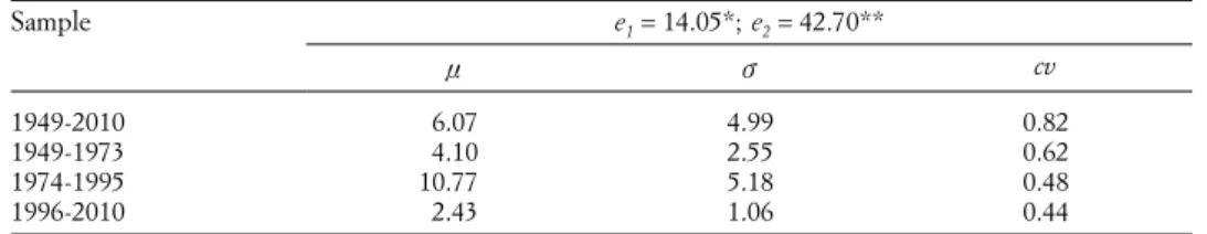
Table 1 displays average inflation rates (n), their standard deviations (v) and variation coefficients (cv = v/n) for the whole sample and the two sub periods.
The inflation rate was much higher in the 1974-95 sub-sample than in all other sub-samples, an outcome that is consistent with the intensity of fiscal dominance, social conflict, union bargaining power and exchange-rate tur-bulence in that period. Inflation volatility was also quite high, whereas the last fifteen years witnessed a dramatic shift to the lowest and most stable val-ues of the sample. Table 1 also shows the results of the Jarque - Bera (1987) (e1) and Doornik - Hansen (1994) (e2) normality tests that evaluate whether asymmetry and kurtosis of the series (over the full sample) conform to those of a normal distribution7. There is clear evidence against the null of
normal-ity for the entire sample.
It is interesting to compare these stylized facts about Italian inflation with those for the United States and the United Kingdom. The latter is a small, open economy very similar in size to Italy; like Italy, it has a long history of changes in monetary arrangements and a rich evolution of labor-market institutions. Figure 3 plots the annual inflation rates (all based on the price deflator of national income) of the three countries, while Table 2 reports
7 The Jarque and Bera test has low power in small samples; the Doornik and Hansen test
corrects for this bias.
TAB. 1. Italy, summary statistics on annual inflation rates
Sample e1 = 14.05*; e2 = 42.70** n v cv 1949-2010 6.07 4.99 0.82 1949-1973 4.10 2.55 0.62 1974-1995 10.77 5.18 0.48 1996-2010 2.43 1.06 0.44
Inflation is defined as the log change of the implicit price deflator of national income. Mean (n), standard deviation (v), coefficient of variation (cv), normality tests (e1 and e2).
simple means and standard deviations of inflation rates over the two halves of our sample. Italian inflation has by far the highest mean and volatility. UK and Italian inflation rates are substantially higher and show a higher degree of persistence than US inflation rate, especially in the 1970s and the 1980s. However, after 1979 the UK and Italian experiences diverge, with the United Kingdom able to mop up inflation much faster than Italy.
The economic significance of these differences may be better understood if they are placed within the institutional context of the three countries. Ital-ian and UK industrial relations were strikingly similar up until Mrs. Thatcher came to power in 1979: her government set monetary stability and low in-flation as a priority. Legislation produced by the Thatcher’s government gradually reduced the national role of unions and collective bargaining (Vis-ser - Ruysseveldt, 1996). Union representation and strike frequency declined sharply to well below the European average. On the other hand, UK mon-etary authorities experimented with several institutional arrangements aimed at reining in inflation, such as monetary targeting and a period of «shadow-ing the deutschemark».
TAB. 2. US, UK and Italian annual inflation rates, 1949-1998. Means and standard deviations
Sample Italy USA UK
mean SD mean SD mean SD
1949-2010 6.072 4.993 3.415 2.218 5.412 4.054 1949-1973 4.101 2.551 2.877 1.953 4.793 2.870 1974-1998 9.902 5.444 4.564 2.433 7.465 4.910 1999-2010 2.178 0.883 2.149 0.802 2.427 0.657 1950 1955 1960 1965 1970 1975 1980 1985 1990 1995 2000 2005 2010 17.5 15.0 12.5 10.0 7.5 5.0 2.5 0
ITAINF UKINF USINF
The US structure of trade unionism was similar to the United Kingdom’s: only few unions were outside the umbrella of the American AFL-CIO or the British TUC. In Italy, in contrast, significant union power was lodged outside the major labor confederations, which were divided along political, organi-zational, and religious lines. In the United States and the United Kingdom, despite declining membership, unions were able to raise members’ wages substantially above non-union wages. In Italy, in contrast, wage settlements spilled over onto the non-unionized sector with the consequence that there was no significant union wage differential8. National labor agreements had
the force of law. Unions were strong and closely tied to political parties; their members were relatively homogeneous. In contrast, the employers’ associa-tion Confindustria was not rooted in a «dense» instituassocia-tional framework and had a membership with relatively heterogeneous objectives. These objectives differed along several dimensions, such as size of firms, industrial sectors, and regional location of firms.
Italy did not go through radical policy changes similar to those experi-enced in the United Kingdom. A system of centralized wage bargaining re-mained at the core of Italian industrial relations, an equilibrium outcome stemming from the interplay of strong political parties, weak governments (Visser, 1998) and a fiscally dominated monetary policy. Macroeconomic in-stability manifested itself with a high and volatile inflation, accompanied by exchange rate devaluations and currency crises. It is no surprise that under such circumstances the identification of a stable tradeoff between output and inflation is a challenging, if not outright impossible, task.
The validity of our key empirical results crucially depends on the unit-root properties of the inflation rate. To assess them, we now consider the conventional Augmented Dickey-Fuller (ADF) test for I(1) against I(0), as provided by evaluation of the t statistic of the bt coefficient in:
u 1 1 t t i i n t i r a nx br c r D = + + - + D + =
-/
,where x is a deterministic trend. A significant statistic implies rejection of the null hypothesis of unit root (H0 : b = 0) and therefore stationarity of the
inflation rate. Table 3 shows results for the full sample and for the two sub-periods demarcated by the split in 1973; we include t-values for the b coef-ficient for both the model with only a constant and with a constant and a trend, each estimated with n = 39.
The very few significant t statistics (in the early part of the sample) do
8 Time series evidence for the 1970s and the 1980s from both the United States and the
United Kingdom suggests that the union differential in the United States was 18%, higher on average than the UK 10% (Blanchflower - Bryson - Forth, 2007).
9 The critical values for this procedure depend on the inclusion of the constant or of the
constant and a trend term. The critical values employed are from MacKinnon (1991). A statis-tic significant at the 5% is marked by *, at the 1% by **.
not cloud the overall result that the test fails to reject the null of a unit root in both models: the inflation rate appears to be a non-stationary process. This highlights that Italian inflation is remarkably persistent, likely because of pronounced macroeconomic volatility. Volatility, in turn, reflects complex forces operating in the economy, such as monetary and fiscal policy regimes and their interdependence, as well as exogenous shocks interacting with the macroeconomic structure. The above result also corroborates the notion that the statistical properties of inflation are likely to change over time. How-ever, based on simple unit root tests we cannot determine the nature and frequency of the structural changes that are responsible for non-stationarity. Moreover, ADF tests have low power in small samples and in the presence of variables containing moving-average components (Maddala - Kim, 1998). To account for this problem, we employed the non-parametric correction to the t-test statistic implied by the Phillips - Perron test, which is more robust with respect to unspecified autocorrelation and heteroscedasticity in the dis-turbance process of the test equation. The results are very close to those of the ADF test10.
These clear findings, while pointing to inflation being an I(1) process, provide the motivation from shifting our focus from the unit-root proper-ties of the series to the possible presence of structural breaks. To this end, we perform a series of tests of multiple structural changes, as proposed by Bai - Perron (1998; 2003; see also Qu - Perron, 2006). This type of test is particularly suited to our case because, among other things, it is designed to evaluate multiple structural breaks in the context of OLS models. It pro-vides a way of testing, using a Sup Wald-type test, the null hypothesis of no change in the coefficients versus an alternative containing a finite number of shifts. Furthermore, Bai and Perron’s algorithm permits to test the null of
m changes versus the alternative hypothesis of m + 1 changes. We apply the
tests to an AR specification with a constant, also accounting for serial corre-lation and different variances in the residuals.
As shown in Table 4, the SupFT(i) tests are all significant for i between 1 and 5; therefore, at least one break is present. The SupFT(3/2) test generates a value of 53.69 that is significant at the 1% level. The sequential procedure
10 Detailed output from the test is available upon request.
TAB. 3. Italy, Augmented Dickey-Fuller test on inflation rates, various sub-samples
Inflation sample
Constant* Constant and trend
i = 0 i = 1 i = 2 i = 3 i = 0 i = 1 i = 2 i = 3
1949-2010 –1.77 –2.03 –1.39 –1.36 –1.77 –2.09 –1.45 –1.43
1949-1973 –3.39* –2.78 –1.73 –1.75 –3.87* –3.04 –1.99 –2.24
1974-2010 –0.64 –1.00 –0.80 –1.08 –2.86 –3.21 –2.98 –3.36
Inflation is defined as the change in the natural log of the implicit price deflator of national income. * indicates rejection of the null with a 95% confidence interval.
and the information criteria (both the BIC and the modified Schwarz crite-rion) all point to three breaks. The inference is that significant shifts in the inflation mean span across at least four intervals; under global minimization the breakpoints are estimated to occur in 1972, 1982 and 1991, all with very narrow confidence intervals. This evidence, which is consistent with our de-scriptive analysis, is likely to emerge from the fact that we have allowed for different residual variances across intervals11. Our sub-samples are
presum-ably also characterized by different degrees of inflation persistence, making our task of giving a structural interpretation to Italian inflation particularly challenging.
This evidence, together with the time-series properties of inflation, sup-ports the conjecture that over our sample period the covariance between in-flation and real economic activity underwent significant shifts. This reason plus the fact that in our relatively long sample we do not have consistent and sufficiently long data beyond prices, output, money and unemployment, make it unworkable to pursue a system estimation. While we acknowledge that a DSGE or a VAR, as in Dees et al. (2009), or a full-fledged cointe-gration with VECM estimation, as in Golinelli (1998)12, facilitate inference
in data-rich contexts, for our study of the annual inflation-output tradeoff a parsimonious single-equation approach is in practice the only robust option.
11 It follows that we allow for a stochastic trend instead of a deterministic one.
12 DSGE stands for dynamic stochastic general equilibrium, VAR for vector
autoregres-sion, and VECM for vector error correction model.
TAB. 4. Tests of multiple structural change of inflation: 1949-2010
Tests SupFT(1) 29.30* SupFT(2) 105.02* SupFT(3) 112.02* SupFT(4) 84.87* SupFT(5) 74.50* UDmax 112.02* WDmax 151.37* SupFT(2/1) 55.43* SupFT(3/2) 53.69* SupFT(4/3) 6.37 Number of breaks selected
Sequential 3 LWZ 3 BIC 3 Estimates of the model with 3 breaks
1 tt 3.84 (0.44) 2 tt 15.63 (0.68) 3 tt 8.28 (0.83) 4 tt 2.81 (0.28) Tt1 1972 (1971:1973) Tt2 1982 (1981:1983) Tt3 1991 (1990:1992) The table presents results of the tests proposed by Bai - Perron (1998; 2003) on an autoregres-sive model of inflation, where the ts denote the coefficients of the lags of the dependent variable. The SupFT(i) tests allow for the possibility of serial correlation in the disturbances. The HAC covariance
ma-trix is constructed according to Andrews (1991) and Andrews - Monahan (1993) using a quadratic kernel with automatic bandwidth selection based on an AR(1) approximation. The residuals are pre-whitened using a VAR(1). We use a 5% size for the sequential test. In parentheses are the standard errors (robust to serial correlation) of the estimated coefficients and the 95% confidence intervals for the break dates.
4. A Phillips curve for Italy?
To evaluate a Phillips-type relationship for postwar Italy, it is best to put it into the context of the literature on the inflation-output tradeoff13. A first
strand blends the classical expectation-augmented Phillips curve hypothesis (Phelps, 1967; Friedman, 1968) with more recent proposals featuring persis-tence and price-wage rigidity (Woodford, 2003). A reduced-form equation of the tradeoff between inflation and output is given by equation (1):
(1) rt=c(yt-y*t)+Et-1rt,
where yt- *yt denotes the output gap14, that is, the difference between the
current level of output and its NAIRU or equilibrium level, and Et – 1rt the expected inflation rate, conditional on last period’s information. The Et – 1rt term embeds a rational expectations hypothesis in a structural model of price rigidity. Equation (1) implies that: unexpected changes in aggregate demand affect both inflation and output; parameter c, defining the slope of the curve, declines as prices become stickier; and the SM mechanism also reduces c, making it zero (a perfectly horizontal curve) when indexation is complete.
The literature has often discussed a forward-looking specification of eq. (2): (2) rt=c(yt-y*t)+bEtrt+1.
Unlike (1), (2) makes the curve shift in response to revisions of cur-rent expectations of future inflation. However, from an observational point of view, the difference between (1) and (2) is not so significant given that expected inflation rates display a high degree of serial correlation. Recently, some consensus has emerged on a specification that accounts for inertia and nominal rigidities. In the framework commonly defined as the hybrid New Keynesian Phillips curve (NKPC), current inflation reacts to expected future inflation and current real economic activity, proxied by real marginal costs that are empirically measured by income’s labor share. The result is a model where inflation is purely forward-looking. However, empirical evidence con-firms that inflation has a significant degree of inertia (Fuhrer - Moore, 1995; Woodford, 2003; Galì et al., 2005; Cogley - Sbordone, 2008). Building on these findings, most models add lagged inflation on top of a forward-looking
13 What follows is not a complete discussion of the various Phillips hypotheses, but
rather a synthesis of the main empirical features of the literature that are relevant to our in-vestigation; see Cecchetti et al. (2007) and Dees et al. (2009) for concise summaries of the main issues.
14 We use the output gap since it is the variable that appears in standard three-equation
specification15. Finally, given the small/open nature of the Italian economy,
it is appropriate to add the rate of change of import prices r*t to account
for the impact of foreign inflation on the domestic price level, impact that in Italy was exacerbated by the SM mechanism. Based on these considerations, we arrive at our preferred reduced-form equation of the Phillips relationship: (3) rt=bEtrt+1+~rt-1+c(yt-y*t)+dr*t +ft.
The parameters in (3), as for all other specifications, are nonlinear func-tions of the underlying structural parameters.
The most important issue in the modeling of inflation is the decomposi-tion of its dynamics between short-run variadecomposi-tion and long-term trend. Mod-ern macroeconomic theory argues for a close tie at business-cycle frequencies between the trend component and inflation expectations. Various statistical methods are available for the identification of this component, such as fil-tering techniques (Hodrick-Prescott, HP; linear or band-pass filters), out-comes from market surveys, or measures derived from inflation swaps or bond-based break-even inflation rates. These methods have their own draw-backs. Inflation swaps and inflation-linked bonds have too short a history to be useful for us. Filtering techniques are limited by the underlying assump-tions. For example, the two-sided HP filter makes the inflation trend depen-dent on a perfect-foresight hypothesis. Agents’ expectations of inflation are a combination of some trend measure and a random component, with the latter, according to rational expectations, being small and unpredictable. Fil-tering techniques, like almost all other alternative methodologies, violate this orthogonality condition. On the other hand, this condition clashes with the empirical evidence that supports adaptive inflation expectations (Fuhrer - Moore, 1995; Cogley - Sbordone, 2008).
Even more fundamentally, the rational expectations hypothesis underly-ing all reduced-form and DSGE models of inflation imposes that economic agents know the «true» conditional probability distribution of macroeco-nomic outcomes. Given the ubiquitous role played by uncertainty, this as-sumption is, to say the least, troublesome. It is particularly so for macroeco-nomic phenomena that are not stationary ergodic processes, that is, phenom-ena characterized by sustained and unpredictable shifts, caused by institu-tional and behavioral changes that show up in structural breaks of the esti-mated parameters. In sum, the Italian study of the inflation-output tradeoff poses peculiar challenges that cannot be met with conventional approaches. The common approach in the literature is to posit that inflation is station-ary and suitable for an equation like (3) to be estimated with GMM16.
How-15 Price indexation, rule-of-thumb behavior, non-linearities in price-setting mechanisms
and time-varying trend inflation are amongst the theoretical explanations of inflation persis-tence.
ever, in the presence of sustained structural changes, most often one faces the difficulty that there are few or no variables that can be employed to pro-duce more reliable inflation forecasts than those generated by a simple AR(1) model, a fatal flaw for the conventional GMM-based approach17. The same
applies to the widespread use of errors-in-variables techniques to modelling rational expectations of inflation: future actual values are used instead of the expected values, and GMM estimation is again employed as in standard dynamic rational expectations models. But relying on future actual values is tantamount to extracting information from the whole sample. Such a meth-odology would be patently inappropriate in cases like Italian inflation, where there is clear evidence of shifts in the steady state and the presence of a sto-chastic trend. Finally, Del Boca et al. (2010) provide evidence of convexities in the response of inflation to changes in the output gap, which argues for an approach that can treat the impact of nonlinearity.
An ideal methodology would be to estimate a multi-equation model, along the lines of the DSGE literature, or to adopt a VAR or Bayesian per-spective (Dees et al., 2009; Benkovskis et al., 2011). Obvious limitations in our data, on the other hand, would suggest sticking to a parsimonious, single-equation specification, one that would account for structural changes and the impact of nonlinearities. To this end, we selected a comprehensive time-varying parameter (TVP) method (Granger - Jeon, 2008; Kim - Nelson, 2006; Cecchetti et al., 2007)18. TVPs helps to identify the conditional
infla-tion-output tradeoff and the causal links between observed institutional or behavioral changes and structural shifts in the parameters. The model in its general state-space form is as follows (Harvey, 1989; Kim - Nelson, 1999):
(4) c x b e b 1 d T b’ z 1 t t t t t t t t r = + + = + + + + l where e N 0, 2 , 0,z N Q b, ,N a 0 0 0
t. ^ vh t. ^ h . ^ Rh, and xt defines a vector of the model’s explanatory variables. The first equation in (4) is the measurement or observation equation. It is the classical linear regression model except that the parameter vector bt (representing the state variables) is posited to change stochastically according to the transition described in the second equation in (4)19.
17 See also Dees et al. (2009) on this point.
18 Alternatively, one could insert variously defined time trends in the model. The TVP
approach yields much richer evidence about time variation, especially about aggregate demand and inflation expectations.
19 We follow the prior distribution proposed by Doan et al. (1984), which assumes that
changes in the endogenous variable are so difficult to forecast that in the AR(1) process of the unobserved state vector the coefficient of its lagged value is likely to be near unity, while all other coefficients are assumed to be near zero. The prior distribution is independent across
If agents were fully informed and under no uncertainty, all parameters of the prior distribution would be known. If this were really the case, a se-quence of generalized least square regressions would deliver an estimate of the state vector. However, such an approach is extremely inefficient com-putationally. More importantly, we have already discussed why uncertainty about parameters’ true values leads to a systematic update of the parameters’ forecasts. Finally, estimation would have to occur even if only some of the parameters of the prior distribution were unknown, a necessary step to draw any inference about b. All these considerations lead to select the Kalman fil-ter as the best suited to make inferences20.
Summing up, our TVP formulation involves forecasting the optimal state vector in each period, conditional on information available up to the previous period21. The computed filtered estimates of the parameters and the
residu-als for each observation in the sample account for the potential variation over time of the underlying parameters. The methodology presents a number of advantages. First, it handles uncertainty in a straightforward way, as it entails a simple learning process of the model’s coefficients. The uncertainty agents face depends upon the error variance of their past optimal forecast, which in turn is conditional on the joint dynamics of output and inflation. Second, it is methodologically parsimonious, since its implementation requires narrow pa-rameterization compared to, say, multi-equation settings, or alternative state-space models with regime switching. Finally, unlike most existing studies that ignore parameter uncertainty and nonlinearities, our approach endogenizes the realization of disturbances to the inflation-output tradeoff and prevents future information from affecting today’s inflation forecasts.
We base our inferences on two measures of trend inflation. The first uses the Structural Time Series (STS) approach proposed by Harvey (1989); for more details, see Hamilton (1994). STS involves decomposing the original series into trend, recursive stochastic cycles, and irregular components that vary over time, using again the Kalman filter22. This generates a
time-vary-coefficients, so that the mean squared error of the state vector is a diagonal matrix. We as-sume that measurement errors and the disturbances to transition equations are serially and mutually independent.
20 The Kalman filter is a recursive procedure for computing the estimator of a time-t
unobservable component, the state vector, based only on information available up to time t. When the shocks to the model and the initial unobserved variables are normally distributed, the filter also enables to compute the likelihood function through prediction error decomposi-tion (Hamilton, 1989; Kim - Nelson, 1999). Both features are particularly suited for the treat-ment of time variation and uncertainty in the inflation-output tradeoff.
21 Under the normality and the independence assumptions about the disturbances, the
computation of the state vector is done with the Kalman filter.
22 This way, we extract time-varying measures of expected inflation that for each
obser-vation rely only on information available up to the point of estimation. This modelling ap-proach is in line with a plausible learning process by both the central bank and private agents. Moreover, the structural time series models are parsimonious models that have reasonably rich ARIMA processes as their reduced forms.
ing trend based on low-frequency autoregressive and cyclical components of inflation’s DGP, based only on information available up to time t. The sec-ond measure is based on the conventional HP filter23. Figure 4 plots actual
inflation along with trend inflation estimated either using the Kalman filter (STSINF) or HP (HPINF). It is easy to spot the sizeable rise in trend in-flation in the late 1960s, its peak between 1980 and 1983, and the marked decline towards the end of our sample. The two measures of trend inflation display quite different volatility and persistence properties, with STSINF fol-lowing more closely inflation’s short-term dynamics, although with a lag.
We employ the STS approach to measure the output gap to account for changes in productivity and potential output. Time-varying potential output is computed by fitting a univariate model on real GDP. Each observation of the estimated potential output relies only on information available up to the point of estimation. As a robustness check, we also tried alternative measures of the output gap – one provided by the OECD, another estimated with the HP filter and a third estimated with band-pass filters – but found very little qualitative differences in the resulting estimates of the inflation-output trade off. Figure 5 plots our measure of the output gap (STSYGAP) along with in-flation. It shows that Italian output and inflation move in opposite directions
23 We also experimented with polynomial trends, moving averages, the kernel-based
smoother and the natural cubic spline; their overall contribution is not significantly different from the HP-based measure.
1950 1955 1960 1965 1970 1975 1980 1985 1990 1995 2000 2005 2010 17.5 20.0 15.0 12.5 10.0 7.5 5.0 2.5 0
INF HPINF STSINF
FIG. 4. Italy, actual and trend inflation, 1949-2010. Inflation (INF), Hodrick-Prescott (HPINF) and Kal-man-filter based (STSINF) measures of trend inflation.
(full-sample correlation: – 0.22), particularly during major shocks, and hints at a non-standard inflation-output tradeoff.
We subjected STSYGAP, the rate of change of GDP and all other mea-sures of real economic activity to ADF and Phillips-Perron unit root tests. Results (not reported here for brevity but available on request) support un-ambiguously their stationarity. Therefore, while Italian inflation is a I(1) pro-cess, as we have already seen, the output gap is I(0). Thus, it would be ques-tionable to look for cointegration between these two variables.
Benchmark OLS estimates
We compute, as a benchmark, standard OLS estimates of equation (3) over the sample 1949-201024. These estimates, based on the HP and STS
measures of trend inflation respectively, are reported below (t-values, shown in parentheses, are computed using standard errors that are heteroskedastic-ity and serial correlation-consistent [HAC]):
* 0.207 (0.80) 0.698 (2.48) 0.208 (1.61) ( ) 0.048 (1.55) 0.87 E y y R 1 1 2 t t t STS t t t STS t t r = r + r + - + r +f = + - * t
24 The existing literature suggests various ways of estimating the output-inflation tradeoff.
Methods like instrumental variables or GMM, besides the considerations made in this Section, suffers from well-known lack of robustness (Muscatelli et al., 2002).
1950 1955 1960 1965 1970 1975 1980 1985 1990 1995 2000 2005 2010 20 0 5 10 15 –5 INF STSYGAP
0.58 (4.11) 0.419 (3.39) 0.039 ( 0.35) ( ) 0.046 (1.90) 0.90 E y y R 1 1 2 t t t HP t t STS t r = r + r - r f -- + + = + - *t *t t
The use of HP in place of STS-based measure of trend inflation does make some difference for parameter estimates, but the key coefficient, the output gap elasticity, is always statistically insignificant across specifications. As evidence of the high degree of inflation persistence, the coefficient of lagged inflation is significant and sizeable, whilst import prices are barely so. These estimates therefore hint at domestic inflation being highly persistent, not linked to output developments25 and somewhat dependent on imported
inflation, the latter likely reflecting recurrent exchange-rate devaluations of the lira26. The output-gap coefficient is never statistically significant,
regard-less of the filtering methodology employed.
Overall, this evidence is inconsistent with the implications of the standard tradeoff between inflation and output. This does not come as a surprise in light of our evidence that inflation is nonstationary and the likely occurrence of significant shifts in the relationship between inflation and real economic activity.
An additional factor that might have affected the covariance between output and inflation shocks is the particular role played by monetary policy. Fratianni - Spinelli (2001b) report several instances in Italian monetary his-tory in which growth in the monetary base was tied to changes in the Trea-sury’s borrowing requirements. In a famous paper, Lucas (1980) estimated a Phillips-type relationship with money in place of output on US data, since filtered data showed that inflation moves roughly one-for-one with money growth. This implies that inflation could react to changes in the monetary base, regardless of the level of real activity. We re-estimated, therefore, the output-inflation OLS tradeoff by replacing the output gap and imported in-flation with the growth in the Treasury component of the money base (MB-TES), over the sample ending in 1998 (i.e., just before EMU). Below we re-port our estimates:
0.022 ( 0.06) 0.828 (2.27) 10.892 (2.46) 0.85 E MBTES R 1 1 2 t t t STS t t r = - r r D f -+ + + = + - t
25 Using the first difference of GDP or industrial production or a HP-based definition of
the output gap does not minimally alter this evidence.
26 Although we cannot rule the impact of imported inflation due to changes in relative
0.552 (3.54) 0.403 (3.85) 7.196 (2.11) 0.88 E MBTES R 1 1 2 t t t HP t t r = r + r + D +f = + - t
Despite the sensitivity of the estimates to the definition of inflation expec-tations, the coefficient of the change in MBTES is positive, sizeable and statis-tically significant across specifications. This is consistent with the fiscal domi-nance view, namely that changes in the monetary base, driven by the accom-modation of the Treasury’s funding needs, exerted a strong impact on inflation.
Baseline time-varying parameter estimates
We now turn to the estimation of a baseline time-varying parameter model for the inflation-output tradeoff, with the aim of shedding some light on the links between institutional changes, such as the SM mechanism and the role of fiscal policy, and the structural shifts in the coefficients of the inflation-output relationship.
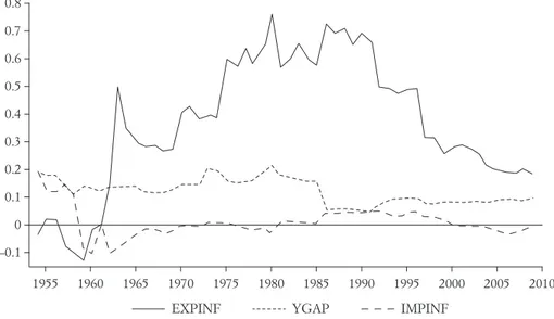
Figure 6 plots the times series of the estimated coefficients of equation (3)27. The estimates were carried out using STS-based measures of trend
in-27 For brevity, we do not show here the full results of our TVP estimation, which are
available from the authors upon request.
1955 1960 1965 1970 1975 1980 1985 1990 1995 2000 2005 2010 0.8 0.1 0.3 0.2 0.5 0.6 0.4 0.7 0 –0.1
EXPINF YGAP IMPINF
FIG. 6. Italy, coefficient estimates of eq. (3), 1951-2010. TVP coefficients obtained using STS-based meas-ures of expected inflation and output gap.
flation and of the output gap28. The behavior over time of the estimates
cor-roborates the hypothesis that the inflation rate and the output gap are only weakly positively associated over most of the sample, with even a few years of negative association, albeit statistically insignificant. This result also ex-plains why standard constant-coefficient techniques detect an insignificant response of inflation from the output gap. Trend inflation and, to a lesser ex-tent, import prices, are more important determinants of actual inflation than cyclical conditions. Figure 7 plots the conditional forecast error variance of inflation, based on our model. It is a helpful gauge of the uncertainty as-sociated with inflation, in part due to the volatility of the equation residual and in part to the evolution in the model’s coefficients. The figure shows that episodes of high inflation uncertainty occurred in the early 1960s, the 1970s, the 1980s and at the onset of the 2007-2009 crisis. The early 1960s were characterized by the «Italian economic miracle», the 1970s and 1980s by oil shocks, the monetization of fiscal deficits, the enlargement of the SM indexation mechanism and later by its removal.
The vigorous output dynamics of the 1950s and early 1960s were largely non-inflationary, as rapid productivity gains pushed outward the Italian economy’s production frontier, while Bretton Woods’ fixed exchange rates shielded the economy from monetary and other nominal shocks. This
ef-28 Employing HP filter-based measures of the output gap does not qualitatively alter the
results. 1955 1960 1965 1970 1975 1980 1985 1990 1995 2000 2005 2010 14 12 10 8 6 4 2 CONDVAR
fect faded out over time. Stronger labor unions, compliant governments, and distorted monetary policy, as we have discussed above, imposed severe con-straints on firms. This assessment is consistent with the central message of Modigliani - Tarantelli (1976), who showed that starting with 1968 deteriorat-ing industrial relations were responsible for an upward shiftdeteriorat-ing and an ever steeper Phillips curve (defined in terms of inflation and unemployment)29.
We estimate a further version of the inflation equation in which, as in the OLS-constant-coefficient case, we replace the output gap and import prices with the growth in the Treasury component of the money base (MBTES), over the sample ending in 1998. The three panels in Figure 8 plot the re-sulting output-gap coefficient estimate (top chart), the implied conditional forecast error variance of inflation (middle chart), and the rate of growth of MBTES (bottom chart). The relevance of Treasury-caused money growth for inflation is confirmed by the size and dynamics of TVP coefficient estimates and by the high (visual) correlation between the implied conditional variance of inflation and the rate of growth of MBTES.
Finally, we performed a number of robustness checks on the sensitivity of our results to the underlying assumptions of the estimated models. First, we reestimated both the conventional OLS and TVP models using alterna-tive definitions of the output gap (HP, linear and band-pass filters, recursive whenever possible; industrial production in place of national income) and trend inflation (HP-based, polynomial trends, moving averages, kernel-based smoother and natural cubic spline). Although in a few cases the findings de-parted quantitatively from the baseline results we have reported, qualitatively the alternative formulations did not make a significant difference. Next, we estimated equation (3) and its variants using GMM, in conformity with much of the international literature and standard dynamic rational expectations models. Overall, the findings were not significantly different from the OLS benchmark. Both GMM and OLS suffer from the shortcomings of imposing the assumption of constant coefficients and no structural changes.
6. Concluding remarks
It is almost heroic to establish a statistically significant response of Italian inflation to the level of real activity in postwar Italy. When we measure the output impact on inflation via standard constant-coefficient techniques, this im-pact is statistically insignificant, possibly reflecting a statistically significant but negative correlation between output and inflation in the early part of the sam-ple and a muted correlation in the latter part. This behavior has its likely roots
29 It should be noted that in a later work Tarantelli (1978) argued that stagflation did not
necessarily hamper the theoretical validity of a textbook-like Phillips curve, especially if the reaction of monetary policy to the resulting cost-push inflation was deflation. However, such reaction does not seem to have materialized up until the end of our sample.
10 5 15 0 BETA DMBTES 1955 1960 1965 1970 1975 1980 1985 1990 1995 2000 10 5 20 15 1955 1960 1965 1970 1975 1980 1985 1990 1995 2000 CONDVARM 1955 1960 1965 1970 1975 1980 1985 1990 1995 2000 0.2 0.4 0 DMBTES
FIG. 8. Italy, TVP estimates, 1951-1998. Coefficient estimate (top chart), implied conditional forecast er-ror variance of inflation (middle chart), rate of growth of MBTES (bottom chart). TVP coeffi-cients were obtained using STS-based measures of expected inflation.
in output and inflation moving in opposite directions during major shocks and in inflation expectations being insignificant in driving current inflation. The exception to this pattern occurs in the period between the 1950s and the early 1960s, when output dynamics were largely non-inflationary, by virtue of rapid productivity gains, and the economy was shielded by nominal shocks, by virtue of the Bretton Woods system. These findings broadly confirm that the stan-dard tradeoff between inflation and output growth emerges only during pe-riods of low inflation and relative macroeconomic stability, as shown, among others, in the comprehensive study by Benkovskis et al. (2011), using time-varying VAR techniques, traditional macro models, as well as DSGE models. We have argued that the Italian «distinctiveness» rests on two institu-tional mechanisms: a rigid wage bargaining process coupled with an index-ation scheme aimed at protecting real wages; and a monetary policy driven by dominant and profligate governments. These forces were the engine of persistent macroeconomic instability.
References
Andrews D.W.K. (1991), Heteroskedasticity and Autocorrelation Consistent Covari-ance Matrix Estimation, Econometrica, vol. 59, no. 3, pp. 817-858.
Andrews D.W.K. - Monahan C.J. (1992), An Improved Heteroskedasticity and Auto-correlation Consistent Covariance Matrix Estimator, Econometrica, vol. 60, no. 4, pp. 953-966.
Bai J. - Perron P. (1998), Estimating and Testing Linear Models with Multiple Struc-tural Changes, Econometrica, vol. 66, no. 1, pp. 47-78.
— (2003), The Computation and Analysis of Multiple Structural Change Models,
Journal of Applied Econometrics, vol. 18, no. 1, pp. 1-22.
Benati L. (2007), The Time-Varying Phillips Correlation, Journal of Money, Credit
and Banking, vol. 39, no. 5, pp. 1276-1283.
Benkovskis K. Caivano, M. D’Agostino A. Dieppe A. Hurtado S. Karlsson T. -Ortega E. - Varnai T. (2011), Assessing the Sensitivity of Inflation to Economic Activity, ECB Working Paper no. 1357, mimeo.
Blanchflower D.G. - Bryson A. - Forth J. (2007), Workplace Industrial Relations in Britain, 1980-2004, Industrial Relations Journal, vol. 38, no. 4, pp. 285-302. Cella G.P. - Treu T. (Eds.) (1998), Le nuove relazioni industriali. L’esperienza italiana
nella prospettiva europea, Bologna, Il Mulino.
Cecchetti S.G. - Hooper P. - Kasman B.C. - Schoenholtz K.L. - Watson M.W. (2007), Understanding the Evolving Inflation Process, U.S. Monetary Policy Fo-rum 2007, University of Chicago Graduate School of Business, The Initiative on Global Financial Markets, mimeo.
Cogley T. - Sbordone A.M. (2008), Trend Inflation, Indexation and Inflation Persist-ence in the New Keynesian Phillips Curve, American Economic Review, vol. 98, no. 5, pp. 2101-2116.
Dees S. - Pesaran M.H. - Smith L.V. - Smith R.P. (2009), Identification of New Key-nesian Phillips Curves from a Global Perspective, Journal of Money, Credit and
Del Boca A. - Fratianni M. - Spinelli F. - Trecroci C. (2010), The Phillips Curve and the Italian Lira, 1861-1998, The North American Journal of Economics and
Fi-nance, vol. 21, no. 2, pp. 182-197.
Doan T. - Litterman R. - Sims C. (1984), Forecasting and Conditional Projections using Realist priori Distributions, Econometric Reviews, vol. 3, no. 1, pp. 1-100. Doornik J.A. - Hansen H. (1994), A Practical Test for Univariate and Multivariate
Normality, Discussion Paper, Nuffield College, mimeo.
Flora A. (1983), State, Economy and Society in Western Europe 1815-1975, vol. I, Frankfurt, Campus.
— (1987), State, Economy and Society in Western Europe 1815-1975, vol. II, Frank-furt, Campus.
Fratianni M. - Spinelli F. (2001a), Storia Monetaria d’Italia, Milano, EtasLibri. — (2001b), Fiscal Dominance and Money Growth in Italy: The Long Record,
Ex-plorations in Economic History, vol. 38, no. 2, pp. 252-272.
Friedman M. (1968), The Role of Monetary Policy, American Economic Review, vol. 58, no. 1, pp. 1-17.
Fuhrer J.C. - Moore G.R. (1995), Inflation Persistence, Quarterly Journal of
Econom-ics, vol. 110, no. 1, pp. 127-159.
Gali J. - Gertler M. - Lopez-Salido D. (2005), Robustness of the Estimates of the Hybrid New Keynesian Phillips Curve, Journal of Monetary Economics, vol. 52, no. 6, pp. 1107-1118.
Golinelli R. (1998), Fatti stilizzati e metodi econometrici «moderni»: una rivisitazio-ne della curva di Phillips per l’Italia (1951-1996), Rivista di Politica Economica, vol. 14, no. 5, pp. 411-446.
Granger C.W.J. - Jeon Y. (2008), The Evolution of the Phillips Curve: A Modern Time Series Viewpoint, University of California, San Diego, mimeo.
Hamilton J. (1994), Time Series Analysis, Princeton, Princeton University Press. Harvey A.C. (1989), Forecasting, Structural Time Series Models and the Kalman Filter,
Cambridge, Cambridge University Press.
Jarque C.M. - Bera A.K. (1987), A Test for Normality of Observations and Regres-sion Residuals, International Statistical Review, vol. 55, no. 2, pp. 163-172. Kim C.J. - Nelson C.R. (1999), State-space Models with Regime Switching,
Cam-bridge, Mass, MIT Press.
— (2006), Estimation of a Forward-looking Monetary Policy Rule: A Time-varying Parameter Model Using ex post Data, Journal of Monetary Economics, vol. 53, no. 8, pp. 1949-1966.
Lucas R.E. (1980), Two Illustrations of the Quantity Theory of Money, American
Economic Review, vol. 70, no. 5, pp. 1005-1014.
MacKinnon J.G. (1991), Critical Values for Cointegration Tests, in Engle R.F. - Granger C.W.J. (Eds.), Long-run Economic Relationships, Oxford, Oxford Uni-versity Press, pp. 267-276.
Maddala G.S. - Kim I.-M. (1998), Unit Roots, Cointegration and Structural Change, Cambridge, Cambridge University Press.
Manacorda M. (2004), Can the Scala Mobile Explain the Fall and Rise of Earnings Inequality in Italy? A Semiparametric Analysis, 1977-1993, Journal of Labor
Eco-nomics, vol. 22, no. 3, pp. 585-613.
Micheletti S. - Spinelli F. (2001), Introduzione all’Inflazione Italiana: 1861-1998, Brescia, Edizioni Ori Martin.
Mitchell D. (1992), International Historical Statistics: Europe 1750-1988, London, Macmillan.
— (1993), International Historical Statistics: The Americas 1750-1988, London, Mac-millan.
Modigliani F. - Tarantelli E. (1976), Forze di mercato, azione sindacale e la curva di Phillips in Italia, Moneta e Credito, aprile-giugno, pp. 165-197.
Modigliani F. - Padoa-Schioppa T. (1978), The Management of an Open Economy
with «100% Plus» Wage Indexation, Essays in International Finance, no. 130,
Princeton, N.J., Princeton University.
Muscatelli A. - Tirelli P. - Trecroci C. (2002), Does Institutional Change really Mat-ter? Inflation Targets, Central Bank Reform and Interest Rate Policy in the OECD Countries, The Manchester School, vol. 70, no. 4, pp. 487-527.
Pellizzari M. (2009), Wage Compression and Self Employment: Evidence from the Abolition of the Scala Mobile in Italy, mimeo.
Phelps E.S. (1967), Phillips Curves, Expectations of Inflation and Optimal Unem-ployment over Time, Economica, vol. 34, no. 135, pp. 254-281.
Sargent T. - Wallace N. (1981), Some Unpleasant Monetarist Arithmetic. Federal Re-serve Bank of Minneapolis, Quarterly Review, vol. 5, no. 3, pp. 1-17.
Spinelli F. - Trecroci C. (2008), The Lira’s Purchasing Power from Italy’s Unification to the Single European Currency, Journal of European Economic History, vol. 37, nos. 2-3, pp. 497-524.
Stock J.H. - Watson M.W. (2007), Why Has U.S. Inflation Become Harder to Fore-cast?, Journal of Money, Banking and Credit, vol. 39, no. 1, pp. 3-33.
Tarantelli E. (1978), Il ruolo economico del sindacato e il caso italiano, Bari, Laterza. van Visser J. - Ruysseveldt J. (1996), Industrial Relations in Europe: Traditions and
Transitions, Sage Publications.
Woodford M. (2003), Interest and Prices: Foundations of a Theory of Monetary Policy, Princeton, Princeton University Press.
Summary: Macroeconomic Instability and the Phillips Curve in Italy (J.E.L. E31, E32, J50, N10) The theme of this paper is whether there was a textbook-like inflation-output tradeoff in post-WWII Italy. We estimate both standard and time-varying parameter models of the relationship between inflation and the level of real economic activity over the 1949 to 2010 period and find no evidence of a stable, significant and positive association between output and prices. We attribute this evidence primarily to a fiscally dominated monetary policy and a rigid indexation mechanism aimed at protecting wages from inflation. These two institutions contributed to the persistent inflation bias and macroeconomic instability that lasted almost until the entry of the country in the European Monetary Union.