Image partition and video segmentation using the Mumford-Shah functional

(1)

Università degli Studi di Salerno

Dipartimento di Ingegneria Elettronica ed Ingegneria Informatica

Dottorato di Ricerca in Ingegneria dell’Informazione X Ciclo – Nuova Serie

TESI DI DOTTORATO

Image partition and video

segmentation using the

Mumford-Shah functional

CANDIDATO:

ALFREDO CUTOLO

TUTOR:

PROF. GIULANO GARGIULO

CO- TUTOR:

PROF. ABDELAZIZ RHANDI

COORDINATORE:

PROF. ANGELO MARCELLI

(2)

(3)

To Mariarosaria and my Parents

(4)

(5)

Introduction

The aim of this Thesis is to present an image partition and video segmentation procedure, based on the minimization of a modified version of Mumford-Shah functional. Generally, in most image processing applications, an image is usually viewed as a set of pixels placed on a rectangular grid. A single pixel provides an extremely local information making impossible any kind of interpretation.

The proposed approach, instead, follows a region based image representations. This approach is used, for instance, in MPEG-4 [27] or MPEG-7 [85] standards. In such cases the image is understood as a set of objects. Region-based image representations offer two advantages with respect to the pixel based ones: the number of regions is lower than the number of original pixels and regions represent a first level of abstraction with respect to the raw information.

The basic objects used of the image partition procedure are the upper and lower level sets of the image. In order to have a more local description of it, we deal with the connected components of (upper or lower) level sets. As proposed by Caselles et al. in [23], we have considered the boundary of these sets, that is the level lines, forming the topographic map.

To be able to handle discontinuous functions, more specifically, upper semicontinuous ones, we define level lines as the external boundary of the level sets of the image. This leads us to the notion of shape which consists in filling the holes of the connected components of the level sets, upper or lower, of the original image. The operation of hole filling was called saturation in [1], [68]. Thus, level lines are the boundaries of shapes and to give the family of level lines is equivalent to give the family of shapes.

Moreover, the family of connected components of upper level lines has a tree structure. And the same happens for the family of connected components of lower level lines. These two trees can be merged in a single tree: the “Tree of Shapes” of an image [69]. It gives a complete and non-redundant representation of the image and is

(8)

contrast independent. The tree is equivalent to the image: its knowledge is sufficient to reconstruct the image.

The image partition procedure determined by level lines is based on the minimization of a simplified version of the Mumford - Shah functional. If we minimize the functional with respect to all possible partitions, the problem of finding a global minimum is exponentially complex. But, if the minimization takes place in a hierarchy of partitions, global minima can be obtained quickly [43] [40].

To build the hierarchy of partitions the tree of image shape has been used. In particular the regions determined by level lines are taken as an initial partition of a hierarchy which can be constructed using the simplified Mumford-Shah functional. Then, using Guigues optimization algorithm [43], the global minima of the energy in the hierarchy can be defined at any scale obtaining the searched image partition.

The Mumford-Shah functional used for image partition has been then extended to develop a video segmentation procedure. Differently by the image processing, in video analysis besides the usual spatial connectivity of pixels (or regions) on each single frame, we have a natural notion of “temporal” connectivity between pixels (or regions) on consecutive frames given by the optical flow. In this case, it makes sense to extend the tree data structure used to model a single image with a graph data structure that allows to handle a video sequence.

We have developed the appropriate graph pre-computing a dense optical flow of the whole video sequence using any of the methods available in literature. So, we have defined the vertices of the graph as all the video pixels, assigning to each one its corresponding gray level. The edges of the graph are of two kinds: spatial edges and temporal edges. Spatial edges join each pixel with its 8-neighbors on the same frame. Temporal edges are defined using the pre-computed optical flow.

The video segmentation procedure is based on minimization of a modified version of a Mumford-Shah functional. In particular the functional used for image partition allows to merge neighboring regions with similar color without considering their movement. Our idea has been to merge neighboring regions with similar color and similar optical flow vector. Also in this case the minimization of Mumford-Shah functional can be very complex if we consider each

(9)

possible combination of the graph nodes. This computation becomes easy to do if we take into account a hierarchy of partitions constructed starting by the nodes of the graph. The global minima of the functional can be defined at any scale using the same optimization algorithm for the image partition [43] obtaining the video segmentation.

(10)

Plan of the thesis

The thesis is organized as follows:

The first chapter reports the different representations of the topology of the image that can be found in the literature. We address our attention at the tree of shape as the data structure for image representation. This structure allows to reconstruct the original image. In particular we show how is possible to construct it merging the tree of shape of upper and lower level lines of the image. To compute the merging operation has been necessary to define the notation of hole and saturation. Then in Chapter 2 we describe an image partition procedure based on minimization of a Mumford Shah functional. The problem of the quick computation of minima using a hierarchy of partitions constructed on the tree of image shape is faced. The section ends with some experimental results.

In Chapter 3 we revise some aspects of the image sequence formation, and the motion estimation problem. We also review the main optical flow estimation methods known in literature. Last section, Chapter 4, proposes a video segmentation procedure based on the minimization of a modified version of the Mumford Shah functional. We describe the data structure used to handle the video sequence characterized by spatial connections (between pixels or regions of the same frame) and temporal connections (defined by the optical flow vector). The procedure adopted to minimize quickly the functional is presented. At the end we show some experimental results comparing a video segmentation obtained with the simplified Mumford Shah functional for image partition with the new introduced functional.

(11)

Chapter 1 Data

Structure

for

Image

Representation

In this chapter we review some issues related to image representation. Representations based on regions are interesting for many image processing applications. Among them, we emphasize the tree of shapes of an image, which gives a compact structure of the level lines of an image. The level lines are the boundaries of the upper or lower level sets of an image. We revise the main properties of these level sets, and the definition of shapes from them, as well as we derive the tree structure of the shapes.

1.1 Different Image Representations

Image representations can be different depending on their purpose. The raw information, that is the values of the samples, or pixels, is a too low level of representation, and the image must be described with more elaborate models.

For a deblurring, restoration, denoising purpose, the representations based on the Fourier transform are generally the best since they rely on the generation process of the image (Shannon theory), and/or on the frequency models of the degradation as for additive noise, or spurious convolution kernel. However, the Fourier transform is purely frequency oriented and does not give directly any space information. The wavelet theory [59][65], achieves a localization of the frequencies, and, due to the linear structure of the

(12)

images at their smallest scales, the wavelet representation is to date the best representation of the image for compression purpose.

Nevertheless, from the image analysis point of view, frequency based representations do not give the adequate information. Indeed, the Fourier representation is nonlocal and the wavelet representation is sensitive to a translation, rotation or scaling in the image, disabling the recognition of objects independently of the viewpoint. Moreover, both of these representations have quantized observation scales.

Scale-space and edge detection theories propose to represent the images by some significant edges, where edges are defined suitably. The algorithms proceed in general in two steps (which sometimes can be merged): first the images are (linearly or not) smoothed [1][21] and secondly an edge detector is applied to the smoothed image. Edges are detected based on the second order derivatives of the image. The earliest definition of edges is due to Marr and Hildreth [61] and a variant was later proposed by Canny [22]. The scale represents the amount of smoothing prior to edge detection. The first scale-space based on edges is the zero-crossing of the Laplacian across the gaussian pyramid, that is the smoothing is a convolution with a gaussian kernel of varying variance. According to Marr, those zero-crossings represent the “raw primal sketch” of the image, that is the basis on which further vision algorithms should rely, see Marr [60] and Hummel [47]. In general, edges extraction can be formulated as a variational problem, see Nitzberg and Mumford [76], Morel and Solimini [70]. The image is approximated by a function that stands in a class of functions for which edges are properly defined: a famous example of such a class is the family of piecewise constant images having a bounded discontinuity length; in this class, the discontinuities lines of the approximating function are interpreted as the edges, see Mumford and Shah [71]. Then, a balance between how close and how complex the approximation is (e.g., with the previous example, the complexity can be the length of the discontinuity boundary), defines a scaled representation of the image.

Despite the generality of the variational approach, it suffers from the fact that there is no theory that says what the model should be. These representations by the edges have two major drawbacks that have been discussed, see Koenderink [51], Witkin [90] and Mallat [59], but not solved within the scale-space theory. First, the geometric

(13)

representation by the edges is incomplete: it does not allow a full reconstruction of the image, therefore some information has been lost in the process of edge detection. Secondly, the decomposition in scales yields a redundant representation.

Another problem with these approaches is linked to the fact that the image gray level is not an absolute data, since in many cases the contrast is camera dependent, and the optics of the camera is generally unknown, and in all cases hard to measure. This problem can be avoided by working in the morphological framework considering the level set and the level lines.

1.2 Level set and level lines

In natural images, the contrast depends on the type of camera, on the digitization process, due to the gray level quantization, to the lightning... Despite this multiplicity of factors changing the contrast, the perception of the image must remain identical, independent of the screen on which it is displayed. In other words, the contrast information is secondary relatively to the geometric information, and useful mainly for visual convenience.

The invariance under change of contrast has been first stated as a Gestalt principle by Wertheimer [89].

Matheron [62] and after him Serra [80], [81] propose a “morphological” representation of the images by their level sets. It yields a complete, contrast invariant representation of the image, independent on any parameter. A variant of this representation is proposed by Caselles et al. in [23], by considering the boundary of these sets, that is the level lines, forming the topographic map.

In general a (gray level) image is represented by a function :

u Ω →ℝ defined in a domain Ω∈_{ℝ . The most basic elements of}2 mathematical morphology are the level sets. We call superior level set Ω and inferior level setX uλ of value λ the subset of Ωdefined as

(14)

( )

{

}

( )

{

}

[ ] , [ ] , X u u p u p X u u p u p λ λ

λ

= ≥ = ∈Ω ≥ = < = ∈Ω < (1.1)

The convention to take strict inequality for lower level sets and large inequality for upper level sets is to get consistency results between them, i.e., Ω\ X uλ = X u_λ .

Whereas it is usually of minor importance because we do not mix upper and lower level sets (1.1), it becomes fundamental when we deal with both simultaneously.

Furthermore, topological characteristics extracted from level sets are also morphological. A particular case is the connected components of the boundaries of level sets, which are called level lines. Another case is taking the connected components of level sets, which are used in the following chapter to construct “shapes”.

Our interest about the level sets comes also from the fact that they are a representation of the image. From the lower level sets of an image u, we can recover uby the formula:

{

}

, ( ) inf :

p u p

λ

p X u_λ

∀ ∈Ω = ∈ (1.2) and for the upper level set by the formula:

{

}

, ( ) sup :

p u p λ p X uλ

∀ ∈Ω = ∈ (1.3)

In the last case, thanks to the non strict inequality, the supremum is actually a maximum, since u p( )

p∈X u.

1.3 Image and its topology

Once the image is segmented, one way or another, the resulting topology must be described. The usual notion of segmentation is a partition of the image into connected regions and the relations between these regions are meaningful. The first idea is to encode the

(15)

adjacency relations: we need to know when two regions have a common boundary. The classical way to represent this relation is through a graph, the Region Adjacency Graph (RAG): each region is represented as a vertex in the graph and when two regions are adjacent, an edge links the corresponding vertices, see Rosenfeld [79]. Nevertheless, adjacency is not the only meaningful relation between regions. For example, if two regions are adjacent, the number of connected components of their boundary is not encoded. The solution to this problem would be to add the corresponding number of edges between the two vertices, yielding then a multigraph. More annoying is the problem that the knowledge that a region is a hole inside another region is not contained in the (multi) graph. Gangnet et al. [41], recognizing that these data are missing, propose to add the inclusion structure of contours to the graphs. However, this represents the topology of the image in two graphs, making it uneasy to manipulate. Observing the difficulty to describe the relations between regions in terms of pixels only, Kovalesky in [54] proposes a cell-list representation, adding frontiers between regions as 1-dimensional elements and the junction points of regions of these frontiers as 0-dimensional elements. However, his structure is not a graph, and does not encode more data than the RAG.

Following the direction opened by Kovalesky, Fiorio in [37] uses the same elements to construct its representation as a combinatorial map (see Lienhardt [57]) and exposes an algorithm of linear complexity to construct his representation, the Frontiers Topological Graph. Fiorio emphasizes the fact that the representation must be consistent with the usual topology of the plane, and that it must introduce the minimum number of elements of non maximal dimension to this purpose. In [38], he generalizes to higher dimensions this representation, whereas in [39], he explains how to manipulate the Frontiers Topological Graph, in particular how to update the structure when two regions are merged and how to extract the Frontiers Topological Graph of a subimage, provided the subimage does not cut regions. Unfortunately, these basic operations are not obvious, coming from the fact that the combinatorial map is a fairly complex representation.

(16)

1.3.1 Topology of morphological representation

All these topological representations are based on a segmentation of the image understood as a partition into connected regions. But the basic elements of mathematical morphology, the level sets, do not compose a partition of the image; instead, they are hierarchical, because they are ordered. When talking about whole level sets, this order, the inclusion relation, is total, yielding a very elementary structure, an ordered list. However, it lacks an important feature of the above representations, the locality, or the fact that the atoms of the representation (the level sets) are not connected. Hence comes the need for considering instead the connected components of the level sets.

A fruitful approach is proposed by Ballester, Caselles and Morel in [5], where the atoms are some parts of the connected components of bilevel sets, that is points whose values are comprised between two given thresholds. They are chosen so that when the thresholds are changed in a manner to have an included bilevel, the subpart of the atom remains connected. These atoms are called the maximal monotone sections, and are invariant with respect to contrast change. Their study comes from a successful shape preserving local contrast enhancement algorithm proposed by Caselles et al. in [24] and [26]. However, the relations between these structures are not totally studied, and their efficiency in terms of compactness of the representation remains to be demonstrated.

Cox and Karron [30] explore the structure of the family of connected components of upper level sets in a 3-D image for purposes of coding and visualization of 3-D data. They show that the image can be described as a discrete structure, the tree of criticalities. They call it the Digital Morse Theory, because it is analogous to the Morse theory for continuously defined functions: a Morse function, that is a twice continuously differentiable function, in which the Hessian matrix is non degenerate at critical points, can be described by a tree of criticalities (see Milnor [67]). From discrete data, a three-dimensional array of gray levels, they define the continuous interpolated functions which are topologically consistent with the discrete data and show that they share the same tree of criticalities. Whereas they remark that using the discrete notions of connectedness (there are two: 4 and

(17)

8connectedness in 2-D, 6 and 26 connectedness in 3-D) without reference to the interpolated function can yield inconsistencies when we take the opposite of the image, they do not push this remark to its natural conclusion: upper level sets are not sufficient to describe topologically the image, because they are adapted to light objects, but the dark objects are not well represented in the digital Morse tree.

In a study on numerical functions defined on a rectangle of ℝ , 2 published in 1950, Kronrod [55] avoids this drawback. Indeed, the atoms in his work are connected components of isolevel sets, which are continua. Given such a component K and a neighborhood U of K, if we call open set the family of the connected components of isolevel sets contained in U , the family of all these sets forms a topology on the set of connected components of isolevel sets of the image. The natural map, that with a point of the rectangle associates the connected component of isolevel set containing it, is continuous. Since the square is connected, locally connected and compact, so is the topological space of connected components of isolevel sets. He shows furthermore that no subset of this space is homeomorphic to the circle S1, concluding that this space is actually a tree, in the topological sense. Moreover, he shows that this tree has an at most countable number of leaves and of ramification points, and that the leaves are connected components of isolevel sets not separating the rectangle (they are some regional extrema, but also what he calls concentric singularities), whereas ramification points are those separating the rectangle in at least three parts. He calls this tree the one-dimensional tree of the function and describes the functions which are in the same family as a given one: they are obtained by merging some parts of the tree. In many respects, this construction is remarkable: the family of connected components of isolevel sets is globally invariant under a contrast change, but also under an inversion of contrast (taking the negative of the function), which was the feature lacking to the digital Morse tree. However, from the image representation point of view it suffers from two drawbacks: isolevel sets are sparse and do not represent an object in the image and the tree is not ordered, meaning that there is no actual root. The first drawback is not related to Kronrod work, since his concern was not image analysis, but rather the study of functions, but the second he solves

(18)

only partially, although he does not emphasize the problem: If we fix a point of the square, the components of isolevel sets not containing this point can be ordered relative to this point. What this amounts to do is to isolate some connected component of isolevel set (the one containing the fixed point), and order the other ones relatively to it, giving a rooted tree. From the image analysis point of view, such a construction is not pertinent, since the point is chosen arbitrarily.

In many respects our work is closely related to Kronrod’s one. We do not deal with isolevel sets but with connected components of upper and lower level sets, whose holes we fill. The notion of hole is not without flexibility, and we develop an axiomatic approach of the adequate definitions of hole. The fact we fill the holes permits to mix the upper and lower level sets in the same structure, namely a tree, which is oriented by inclusion. In this manner, the tree describes in a straightforward manner the topology of the image. This is related to Kronrod’s article in the sense that the boundary of our atoms are (connected parts of) connected components of isolevel sets (at least for a continuous function), and that filling the holes of a connected component of upper level set is exactly the same as filling the holes of its boundary (see Proposition 1.18). In this manner, we precise what is the interior of a connected component of isolevel set, this interior being defined with no arbitrary choice, and this orders the atoms by inclusion. This keeps the advantages of Kronrod’s tree, namely contrast and negative invariance properties, while being adapted to image analysis, because most objects in the image are likely to be formed of atoms of our representation. Moreover, we gain generality because the results are valid for a semicontinuous image.

1.4 Tree of shape as an image representation

Now we want to show that, under certain topological conditions concerning the images and their set of definition, the “shapes” have a tree structure. This notion of tree is not the classical one, in the sense that it is not a discrete structure, since it can have an infinite (and possibly not even countable) number of nodes, yet it is consistent with it: two arbitrary nodes are connected, and there is no loop.

(19)

The shapes of an image are built from the connected components of level sets. It is well known that connected components of level sets have a tree structure. The difference here is that we consider simultaneously superior and inferior level sets and the shapes constructed from them are stored in one structure, without redundancy. This may seem paradoxic, since the datum of the connected components of lower level sets, or the datum of the connected components of upper level sets, are each sufficient to reconstruct the image. The explanation of this paradox is that the shapes are not constructed from all those connected components, but from a selection of them, this selection being of course independent of the contrast. Moreover, this selection is consistent with what we expect to be “objects” in the image and discards the background. We do not pretend to solve the foreground-background ambiguity in general, but this ambiguity appearing only for regions meeting the frame of the image, most of the time the good choice is made.

The tree of shapes is complete and without redundancy. What these properties mean is that the datum of the shapes is sufficient to reconstruct the image (completeness) and that it is necessary for this operation (absence of redundancy), in the sense that removing a part of the tree does not permit to reconstruct the image or yields a different image. In these respects, the tree of shapes is a representation of the image. Moreover, we believe this tree is a representation adapted to image analysis, its contrast invariance being not the least of its advantages. Finally, for discretely defined images, a fast algorithm allows the decomposition, the reconstruction being trivial. This is exposed in the next chapter.

1.4.1 Basic definition

Unless otherwise defined, Ω will be any connected topological space. We call image an application from Ω to ℝ . Ω will sometimes need to be locally connected. We recall the definition of local connectedness:

Definition 1.1 A topological space Ω is said to be locally connected if the following equivalent properties hold:

(20)

2. the connected components of any open set of Ω are open; Notice that local connectedness is a property totally independent of the fact that the topology is metric or not.

The notion of connectedness we use is the classical topological one:

Definition 1.2 (Connectedness) A topological space X is said

to be connected if any partition of Ω into two closed sets results in one of them being φ; and the other one Ω. A subset of Ω is said to be connected if it is connected as a topological space (for the induced topology).

This can also be formulated with partitions into two open sets (it is enough to consider the complements), or saying that the only open and closed subsets of Ω are φ and Ω, or in an alternative formulation: the only subsets of Ωhaving φ as boundary are φand Ω. Other notions of connectedness exist, as for example arc-wise connectedness, or strong connectedness, but we restrict the discussion to the classical one.

The two most important basic results that are useful are: 1. The union of a family of connected subsets of Ω

having a nonempty intersection is connected.

2. If C⊂ Ω is connected and C ⊂ ⊂D C, then D is connected.

The first point implies that any topological space can be partitioned in a family of maximal connected subsets, and this decomposition is unique. Its elements are called the connected components. The second point implies that if C is connected, C is connected, and an easy consequence is that the connected components of a set S are closed in S (but not necessarily open, except when S is locally connected, hence the interest of this notion of local connectedness).

It is clear that the family of superior level sets is decreasing, whereas the family of inferior level sets is increasing:

, X uλ X u X uµ , _λ X u_µ

λ µ

(21)

As explained in Section 1.2, each one of these families allowing to reconstruct the image from Equations 1.2 and 1.3.

1.4.2 From level sets to their components

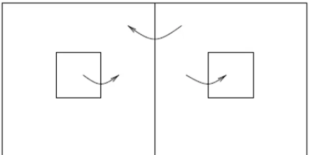
Whereas contrast invariant, level sets are not compatible enough with our visual perception to have any hope of representing visual “objects”. It seems true that the eye is the most at ease in comparing two light intensities (much more than for example in comparing hues), yet these comparisons do not seem to be global: it is able to isolate from two adjacent regions the brighter one, but for non adjacent regions, the comparison does not seem to be reliable (see Figure 1).

Figure 1: Comparing the two small gray squares, the eye is not at ease comparing

their gray level. The left small square might appear brighter than the right one, whereas they have the same brightness.

The consequence is that global comparisons are not meaningful, that is only adjacent regions should be compared. The information left is in Figure 2. The arrows in this figure represent the relation “brighter than”. This relation is transitive, but observe that it does not allow to compare the gray levels of the two squares.

Moreover, any homogeneous region appears as one “object”, that is not split by the eye. This leads us to work with connected components of level sets rather than with the whole level sets. The fact that two regions are connected components of the same level set is not a relevant information, we do not compare their gray level. This is the case for the small gray squares in Figure 1.

(22)

Notation: given a point xin X uλ , let us denote by cc X u p

(

λ ,

)

the connected component of X uλ containing x. By convention, if

(

)

, cc ,

x∉X uλ X u pλ is φ. A similar notation applies to cc

(

X u p_λ ,

)

. We derive evidently from Equations 1.2 and 1.3 the reconstruction formulae:

(

)

{

}

( ) inf | , u p = λ cc X u p_λ ≠φ

(

)

{

}

( ) sup | , u p =

λ

cc X u pλ ≠

φ

The monotonicity of level sets translates into a tree structure for their connected components. Since their number need not be finite, we have to define a more general notion of tree.

Figure 2: the information left from image of Figure 1 when only local comparisons

are performed. The arrows represent the order relation “brighter than”.

Definition 1.3: Let

ε

be a family of sets and ≺ a partial order relation in

ε

. We say that ≺induces a tree structure in

ε

if the two conditions hold:

1. ∃ ∈ ∀ ∈R

ε

, E

ε

, E≺R;

2. A B C, , , A B B and C are comparable .

A C

ε

 ∀ ∈ _⇒  ≺ ≺

The first condition expresses the connectedness of the structure, Rbeing the root of the tree, and the second condition implies that

(23)

there is no loop, because, given four sets A B C D, , , ∈ε , the following situation cannot happen:

. A B D A C D ⊂ ⊂ ⊂ ⊂

B and C not comparable .

A particular case occurs when the relation order is the inclusion of sets, in which case we talk about an inclusion tree.

With this definition we show the tree structure of connected components of level sets.

Proposition 1.4: Let ube an image. Let A=cc X u p( λ , )(resp.

( , )

A=cc X u p_λ ) and B=cc X u p( µ , ) (resp. B=cc X u p( _µ , )). Suppose that A∩ =B φ. Then either A⊂Bor B⊂ A.

Proof. Suppose, without losing generality, thatλ µ≤ . Then we have [u≥µ]⊂ ≥[u λ], thus B⊂ ≥[u λ]. Let z∈ ∩A B, then clearlyA=cc X u z( λ , ), and since B is connected, contains z and is contained in [u≥λ], we deduce that B⊂ A.

The case of the connected components of inferior level sets is dealt with in the same manner. □ This implies (and is stronger than) the inclusion tree structure:

Corollary 1.5: For a bounded image u, the set of lower level sets X u_λ and the set of upper level sets X uλ are each inclusion trees.

Proof: The root is the definition set of u. If A B, and C are lower level sets, A⊂B and A⊂C, we get A⊂ ∩B C, which proves that B∩ =C φ and, using Proposition 1.4, that B and C are comparable for inclusion order. The proof is similar for X uλ . □

1.4.3 Beyond components of level set

The above simple result only is a small extension of Equation (1.4). Nevertheless, it is a substantial improvement over these formulas in the sense that it represents more faithfully the objects in the image. We have got locality, which was one of the main

(24)

motivations of this work. In these two trees, we expect to find the meaningful objects perceived by the eye. In this sense, these trees seem to be useful for image analysis.

The problem with their use is linked to reconstruction. It is acknowledged that the trees are sufficient information to reconstruct the image they are extracted from, but they are redundant. Since each tree represents exactly the image, if we want to deal as well with upper level sets as with lower level sets (which we do), manipulations of these trees is a problem. For example, the basic operation we would like to do on a tree is to remove one node. Since the other tree is not linked (except that it represents the same image initially), it must be extracted again so that it represents again the image of the first tree. There is no quick solution to this; we have to reconstruct the image from the modified tree and extract the other tree. This drawback is due to the lack of link between the two trees. Whereas the inclusion information is encoded for components of the same type of level set in their tree, there is no such information between components f different types of level sets. This is to be expected since such components are not nested, that is we cannot keep an inclusion tree structure with all components of lower as well as upper level sets.

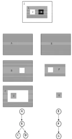
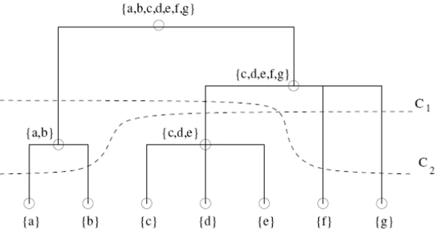
Figure 3 illustrates the fact that both trees can have very different structures. Since no one should be privileged, the use of their tree structure is a problem. This example hints at what is lacking in both trees. The link between them is related to the notion of holes. In this figure, D is an hole in F and this information is interesting from an image analysis point of view.

Since each tree represents exactly the image, the datum of both is at the same time too much (since there is redundancy) and not enough because such relevant information as the relation of being a “hole” in an object does not appear in these data.

All these problems have a common solution: instead of considering connected components of level sets, we work with connected components of level sets whose holes are filled. This elementary operation yields what we call shapes. The shapes keep the same properties as connected components of level sets: locality and insensitiveness to contrast change. The relation between connected components of level sets of different types “is a hole in” translates in this framework to the relation “is contained in”. Fortunately, this

(25)

operation remains consistent with image analysis. Since we live in a world where numerous objects are “full”, a hole in their projection in an image must be due to occlusion, and representing such projections without their holes is faithful to the true object.

The redundancy between the two trees is automatically removed. Taking the example of image of Figure 3, the shapes based on components A , B , C and E are the same: the whole image.

Figure 3: Top: an elementary image with three “objects”: two squares and one rectangle. Left column: the connected components of upper level sets with increasing thresholds from top to bottom. Right column: the connected components of lower level sets with decreasing thresholds from top to bottom. Bottom line: the two associated trees, where arrows represent the relation “contains”. The two squares, which are relevant from an image analysis point of view, are of different types and therefore appear in different trees, showing that both trees are of interest.

(26)

Whereas the square G is included in the rectangle F, there is no link between D and

F.

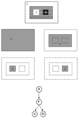
The shapes based on D and G are D and G themselves, since these components have no hole. On the contrary, the component F become the same rectangle F', and D which was a hole in F , is a subset of F'. As shown in Figure 4, the shapes have an inclusion tree structure. In the following section, we investigate the conditions under which a continuously defined image can be represented by a tree of shapes. This will imply the definition of the notion of hole and of the concept of saturation.

Figure 4: The shapes based on the elementary image as in Figure 3. The component F of Figure 3 becomes full here; D and G do not change since they have no hole, and all the other components become A, the whole image. The image is represented by a unique inclusion tree, where upper and lower level sets have equal importance. Notice that reversing the contrast (negating all gray values) would yield the same tree structure.

(27)

1.4.4 Saturation, hole and shape definition.

In this section we want to show that the shapes extracted from an image have an inclusion tree structure and to investigate the possibilities of reconstruction of an image from its shapes. Under these conditions, decomposition of an image into shapes will be a powerful image representation, well adapted to image analysis.

Heuristically, the tree of shapes is a data structure to encode in a tree the family of level lines of the image. To be able to handle discontinuous functions, more specifically, upper semicontinuous ones, we define level lines as the external boundary of the level sets of the image. This leads us to the notion of shape which consists in filling the holes of the connected components of the level sets, upper or lower, of u. The operation of hole filling was called saturation in [1], [68]. Thus, level lines are the boundaries of shapes and to give the family of level lines is equivalent to give the family of shapes. It is easy to imagine them when the image is smooth (its graph is a smooth topography).

Definition 1.6: Let Ωbe a connected topological space and A⊂ Ω. We call hole of A in Ω the components of Ω\ A.

Definition 1.7: Let p_∞∈Ω\A be a reference point, and let T be the hole of A in Ω containing p_∞. We define the saturation of A with respect to p_∞as the set Ω\T and we denote it by Sat A p( , _∞). We shall refer to T as the external hole of A and to the other holes of A as the internal holes. By extension, if p_∞∈A by convention we define Sat A p( , _∞)= Ω. Note that Sat A p( , _∞)is the union of A and its internal holes.

The saturation operator is the operator that transforms the connected components of level sets to “shapes”. This operator fills the holes of the connected components of level sets.

We will denote by ΤAthe set of holes of A and Ext A the exterior

(28)

( ) A T sat A A T ∈Τ = ∪ ∪

where the unions are disjoint.

Notice that the definitions of holes and exterior depend on the saturation operator chosen on Ω. But we will never consider several saturations at the same time, so that the context will be clear enough to disambiguate these notions.

Definition 1.8: Given an image u, we call shapes of inferior (resp. superior) type the sets

(

)

(

,

)

(

.

(

,

)

sat cc X u p_λ resp sat cc X u pλ

We call shapes of u any shape of inferior or superior type. We denote by S u

( )

the family of shapes of u.

Examples of interesting saturation operators will be shown later, but here is a trivial one: consider the operator that transforms φ; to either φ; or Ω and any other set to Ω. This operator destroys all information from the connected components of level sets of an image and inhibits the reconstruction of an image from its shapes, which is one of our concerns.

1.4.5 Saturation of complement

We derive from the definition the essential properties of a saturation operator on a connected topological space Ω.

Definition 1.9: We say that A⊂ Ω is a simple set when A is connected and sat A

( )

=A.

In other words, a simple set is a connected set that has no holes, that is a connected fixed point of sat.

The first result is that a hole in a connected set is a simple set or its saturation is Ω.

(29)

Lemma 1.10: Let A be a connected subset of Ω and T a hole in A. Then either T is a simple set or sat T

( )

= Ω, the last case implying sat A

( )

= Ω.

Proof: T being a connected component of the complement of a connected set

( )

A in a connected space, we know that Ω\ T is connected (see [75], IV.3, Theorem 3.3). So this set is either a hole of T, in which case sat T( )= Ω, or the exterior of T , in which case

( ) sat T =T.

If sat T( )= Ω, then since T ⊂sat A

( )

, the monotonicity of sat yields

( )

(

( )

)

( )

.

sat T sat sat A sat A

Ω = ⊂ =

□ This immediately yields

Corollary 1.11: Let A a connected subset of Ω and T a hole in A . Then sat T( )⊂sat A

( )

.

1.4.6 Properties of saturation

We investigate here the topological properties of simple sets, in particular their position relative to their boundary. It appears that pathological situations are avoided when the space Ω is locally connected (see Definition 1.1). Notice that from the idempotency of the saturation operator simple sets are the image by the saturation operator of some sets, in other words, sets that are already saturated. The converse (i.e., the saturation of a set is a simple set) would be true at the condition this saturated set is connected.

Saturation preserves connectedness

First we prove that saturation preserves connectedness. This will be a direct consequence of the following lemma:

(30)

Lemma 1.12: Let Ω be a connected topological space. Suppose that Ω is locally connected. If A⊂ Ω, Ais connected and T is a connected component of Ω\ A, then A∪Tis connected.

Proof. Suppose that A∪Tis not connected. Then A and T being connected, they are the connected components of A∪T. Thus A and T are closed in A∪T , and each one being the complement of the other one in this space, they are also open. Thus, there is an open set

U in Ω such that T ⊂U and U∩ =A φ. We can suppose U

connected, otherwise it suffices to take the connected component of U that contains A (there is one since A is connected), and this component is open since Ω is locally connected. U is then connected, included in Ω\ Aand contains T . Since T is a connected component of Ω\ A, this implies T =U, an open set.

As T is closed in A∪T T, ∩ =A

φ

, and T being connected, T =T . Since

φ

≠ ≠ ΩT , the fact that T is open and closed is a contradiction with the connectedness of Ω.

This lemma allows us to show the connectedness preserving property of saturation:

Proposition 1.13: Let Ω be a connected and locally connected topological space, sat a saturation operator on Ω and A⊂ Ω a connected set. Then sat A

( )

is connected.

Proof. It suffices to write

( )

(

)

A T sat A A T ∈Τ = ∪ ∪

a union of connected sets (thanks to Lemma 1.12) having a nonempty intersection

( )

A . sat A

( )

is then connected. □

As a consequence of Proposition 1.13, all properties proved below apply to shapes of any image defined on Ω, since shapes are simple sets.

Saturation preserves topology

(31)

Lemma 1.14: Let Ω a connected space, sat a saturation on Ωand A⊂ Ω. If A is open, sat A

( )

is also open. If Ω is locally connected and A is closed, then sat A

( )

is also closed.

Proof. If sat A

( )

= Ω, the assertions become trivial, so we will suppose this is not the case.

( )

\ sat A

Ω is a connected component of Ω\ A, so that it is closed in \ A

Ω , which is closed provided A is open. Thus Ω\ sat A

( )

is closed in Ω, which proves that sat A

( )

is open.

If A is closed, then Ω\ A is open, and Ω\ sat A

( )

is a connected component of Ω\ A, so Ω\ sat A

( )

is open (since Ω is locally connected), proving that sat A

( )

is closed. □

Remark: A direct consequence of Lemma 1.14 is that the only

shapes of an upper semicontinuous image u that are of inferior and superior type are φ and Ω. Indeed, since connected components of upper (resp. lower) connected components of level sets are closed (resp. open since Ω is locally connected), their saturation is also closed (resp. open). Thus a shape being simultaneously of inferior and superior type would be open and closed, the connectedness of Ω implying this shape would be Ω or φ. Remark this becomes false when u is not upper semicontinuous, as shown in Figure 5.

Figure 5: For an image that is not upper semicontinuous, a nontrivial shape can be

of inferior and superior type. In this example, the central disk is approximated by a sequence of decreasing circles at level 2, whereas the gaps between circles are at

(32)

level 0. This disk is a connected component of X u1 u and X u₂ , without holes for the natural saturation of ℝ2.

Boundary of saturation sets

If A is a set in a topological space we denote with A∂ the boundary of A .

We now show that the boundary of the saturation of a set A is a subset of the boundary of A .

Lemma 1.15 If A is any subset of a locally connected space Ω, and

{

A ii, ∈I

}

are its connected components, then

i i I

A A

∈ ∂ ⊂ ∂

∪

Proof. Let i∈I. On one hand, we have:

i i

A A A

∂ ⊂ ⊂ .

On the other hand, Ω\A⊂ Ω\A, so that taking the complement of each member we get

\ \

A⊃ Ω Ω A (*) Then (**) the last inclusion coming from the fact that A_i∩ =A A_i, expressing that A_i is closed in A , since it is a connected component of A . Since

\ \ A

Ω Ω is open and Ω is locally connected, its connected components are also open. Thanks to

( )

* , each connected component of Ω Ω\ \ A is contained in a connected component of A . Therefore,

\ \ A

Ω Ω being moreover open, each one of its connected components is contained in the interior of a connected component of A . Thanks to

( )

** , we get

( )

A_i

(

\ \A

)

A_i

°

∂ ∩ Ω Ω ⊂

which implies that

( )

∂A_i ∩ Ω Ω

(

\ \A

)

=

φ

since

( )

Ai Ai

φ

°

∂ ∩ = meaning ∂ ⊂ ΩA_i \A. □

Remark: w_{ithout additional assumptions, the converse inclusion} is false. Consider as an example Ω =ℝ with the usual topology and

(33)

A=ℚ . Then A∂ = Ω whereas the connected components of A are composed of one rational, thus for each i , A_i =A_i and _i

i

A =A

∪

.

Nevertheless, if I is finite, the fact that the A are connected _i components of A implies _i

i I

A A

∈

=

_∪

which is sufficient to prove the converse inclusion.

Proposition 1.16: If Ω is locally connected and A⊂ Ω, ( )

sat A A

∂ ⊂ ∂

Proof. If sat A( )= Ω, we get ∂sat A( )=φ and the result is trivial. Now suppose that Ω\sat A( )≠φ.

( )

(

)

( ) \

sat A sat A

∂ = ∂ Ω and Ω\ sat A

( )

is a connected

component of Ω\A. Thus,

( )

(

\sat A

)

(

\A

)

∂ Ω ⊂ ∂ Ω

meaning ∂sat A( )⊂ ∂A. □

The next important result links the saturation of a set to the saturation of its boundary.

Lemma 1.17: Let Ω be a topological space and A⊂ Ωbe an open connected set. Then A is a connected component of Ω ∂\ A.

Proof. Since A is open, A⊂ Ω ∂\ Aand moreover

(

\

)

A= ∩ Ω ∂A A

proving that A is closed in Ω ∂\ A, and since it is also open in it and connected, it is a connected component of Ω ∂\ A. □

Proposition 1.18: Let Ω a connected and locally connected topological space and A⊂ Ω such that sat A

( )

≠ Ω. Then

( )

sat A ⊂sat ∂A , and if A is closed, we get sat A

( )

=sat

( )

∂A .

1.4.7 Decomposition of an image into shapes

The above results concerning the properties of the saturation operator are the tools needed to prove that shapes have an inclusion tree structure. Nevertheless, this requires additional assumptions on the space Ω, which, as we will see, are met with ℝ . n

(34)

Our first proposition is the easy part of our general theorem, and does not need further hypotheses about Ω. It compares the saturations of connected components of the same type of level set.

Proposition 1.19: Let Ω be a connected and locally connected space and u an image defined on Ω. Let A and B be two shapes of

u of the same type such that A∩ ≠B φ. Then either A⊂Bor B⊂ A. It deals with the comparison of the saturations of connected components of level sets of different types. Notice that it involves a strong hypothesis on the boundary of the open shape, which explains why additional hypotheses on Ω are required, so that this hypothesis is automatically satisfied for all open shapes. Notice the proposition is formulated in such a way that the two connected components have one point

( )

p in common.

Proposition 1.20: Let u be an upper semicontinuous image on Ω, A=sat cc X

(

λ,p

)

and B=sat cc X

(

_λ,p

)

two shapes of u. Suppose also that B∂ is connected. Then either A⊂Bor B⊂ A.

The following lemma deals with the last case: when the connected components of level sets are disjoint.

Lemma 1.21: Let A and B be two disjoint connected sets of a

connected and locally connected topological space. Then sat A

( )

and

( )

sat B ) are either nested or disjoint.

The following theorem sums up the three preceding results and is the achievement of this section.

Theorem 1.22: Let u be an upper semicontinuous image on the connected and locally connected space Ω, A and B two shapes of u

with connected boundary. Then A and B are either disjoint or nested. From this result, we can conclude that the set of shapes of an (upper semicontinuous) image has an inclusion tree structure. For simplicity, we assume that our image is discrete. Then we can represent the tree as a finite structure; the shapes are the tree nodes and the parent-child relationship, represented by the links between nodes, is determined by inclusion (the child A being a shape contained in the father Af with no other shape B such that

f

(35)

1.4.8 Unicoherent spaces

As we have seen, the shapes of an image have an inclusion tree structure under some restrictive condition on u: that its shapes have connected boundary. Actually this can be ensured from the upper semicontinuity of u if the definition set Ω is unicoherent. We recall the definition of a unicoherent space:

Definition 1.23: A topological space Ω is said to be unicoherent if it is connected and whatever connected closed subsets F and F ' such that X = ∪F F', we have F∩F'is connected.

Let us give an example of unicoherent spaces. ℝ , and any interval I of ℝ , are unicoherent. Indeed, a connected subset of Ω =ℝ or I is an interval. So if Ω is the union of two closed intervals, they intersect and their intersection is a closed interval, thus a connected set. It is harder to prove that ℝ and any hypercube of n

n

ℝ are unicoherent. In particular, the closure of a Jordan domain in

n

ℝ is unicoherent, since it is homeomorphic to a hypercube in n

ℝ .

Proposition 1.24: If Ω is a unicoherent and locally connected space, sat is a saturation on Ω and u is an upper semicontinuous image defined on Ω, then all shapes of u have a connected boundary.

We deduce the following

Corollary 1.25: In a unicoherent and locally connected space Ω

with a saturation, two shapes of an upper semicontinuous image defined on Ω are either disjoint or nested.

1.4.9 Applications

Until now, we have shown that provided some hypotheses on the topological space Ω are true, the shapes of a semicontinuous image defined on Ω have an inclusion tree structure. But the definition of shapes requires that we have a saturation operator on Ω. The goal of this section is to exhibit saturation operators that are relevant to image analysis. We will do this when Ω is a closed Jordan domain in ℝ n (for example a hypercube), for n≥2.

When the image u is defined only on a bounded subset of ℝ , we n would like to have a property similar to Theorem 1.22, where shapes

(36)

should have an easy interpretation in terms of image analysis. The idea is that only a part of an image defined on ℝ is observed. The n first (bad) solution would be to extend the image u to ℝ by an n arbitrary value. The problem is precisely that this value is arbitrary, and different values would give different trees.

We would like that “objects” totally included in the definition set are described in the same manner they would be if the whole image on

n

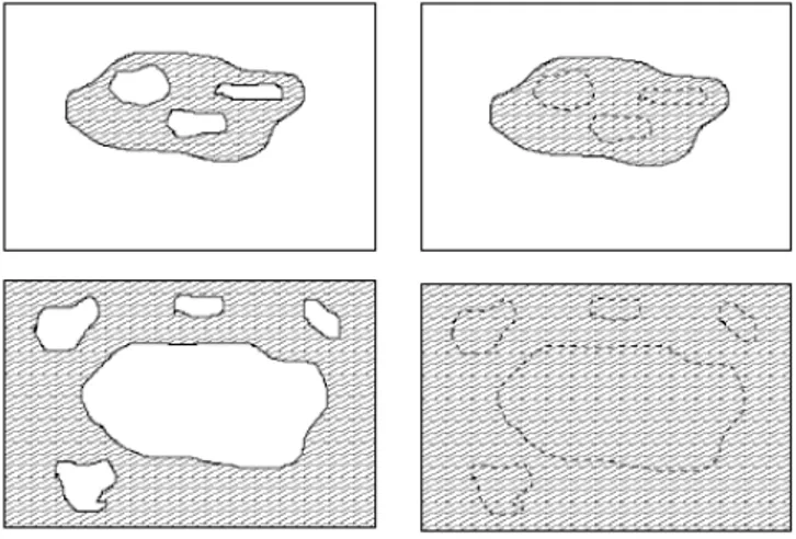
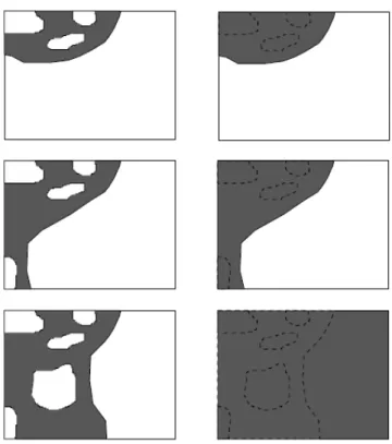
ℝ were observed. So that connected components of level sets not meeting the frame of the definition set are supposed not to be cut. At this condition, whatever the image u outside the definition set, its holes are the components of the complement not meeting the frame. For the same reason, the saturation of a connected set containing the frame is the definition set itself (see Figure 6). There remains to deal with the connected components of level sets that meet the frame without containing it.

Figure 6: Saturation of some sets in a bounded definition set. Left: two sets (dashed) in their respective image. Right: their saturation (dashed). The top-left set does not meet the frame of the image. It is saturated as if the image were infinite (whatever the image outside the definition set, the result is the top-right set). The bottom-left set contains the frame of the image. It is also saturated as if the image were infinite (whatever the image outside the definition set, the result would contain the whole definition set, shown bottom-right). The saturation of a set containing the frame of the image is always the whole definition set.

(37)

The intuitive notion of a hole is that of a connected component of the complement “smaller” than the exterior. When the definition set is

n

ℝ , in some sense a bounded set is “smaller” than an unbounded set, so that we can define the holes and the exterior in agreement with the intuition. When u is defined on a bounded set, we quantify this notion with the help of measure theory. Therefore, we need to suppose that we are provided with a measure on the definition set.

We need moreover this definition set to be unicoherent. This imposes strong constraints. We suppose that Ω is the closure of a Jordan domain in _{ℝ , or more generally in}2 _{ℝ , i.e., the closure of the}n

interior of a subset of _{ℝ homeomorphic to}n n 1

S − . Then we know that Ω is a connected and locally connected subset of ℝn n≥2, and also unicoherent, for the usual topology induced by ℝ . We suppose also n that a Borel measure µ is given on Ω. Therefore, since Ω is compact,

µ

( )

x < ∞. The boundary of Ω as a subset of _{ℝ , denoted}n

by ∂Ω, is called the frame of the definition set; it is a connected set (the Jordan hypersurface).

From these remarks, we define the saturation as follows:

Definition 1.26: Let A a measurable subset of Ω. We define

( )

sat A as:

(

)

{

}

(

)

( )

{

}

\ : \ \ : / 2 A C cc A C ifA if A C cc A C and C if A φ φ φ µ µ φ  _∪ ₌ _Ω _{∩ ∂Ω =} _{∩ ∂Ω =}  Ω ∂Ω ⊂  Ω = Ω ∩ ∂Ω ≠ > Ω ≠ ∩ ∂Ω ≠ ∂Ω    (1.5) The new case is concerned with sets that meet the frame of the image without containing it. The construction of the associated shape is illustrated in Figure 7. That half the area of the image plays a specific role is justified by the fact that this yields a saturation operator.

The fact that we use a Borel measure yields:

Lemma 1.27: If A⊂ Ωis measurable, then every connected component of A and of Ω\ Ais measurable.

We are in a position to prove that the sat operator, as defined in 1.28, is indeed a saturation operator.

(38)

Figure 7: The construction of the shape associated to a set meeting the frame of the

image but not containing it. This is the case that was not illustrated in Figure 6. Left: the sets. Right: the associated shapes. In the first two cases (two first rows), one connected component of the complement has a (Lebesgue) measure larger than half the one of the image, this is the exterior of the set. The other connected components are the holes. In the third case (third row), no connected component of the complement has a sufficient measure, they are all considered as holes and the associated shape is the whole image.

Proposition 1.28: The operator A⊂ Ω of Formula (1.5) is a saturation operator on Ω.

This implies that the shapes (according to the saturation operator of Definition 1.26) of an upper semicontinuous image defined on Ω, the closure of a Jordan domain in ℝn, n≥2, have a tree structure.

(39)

Chapter 2 Image

segmentation

based

on

minimization

of

Mumford-Shah

functional

In this chapter we address the problem of image segmentation. In particular, we introduce a variational approach which use the classical Mumford-Shah functional and is subordinated to the tree of shapes of the image. We carry out the minimization of the functional using a hierarchical processing algorithm. At the end we show some results of segmentation.

2.1 The simplified Mumford-Shah functional on

the Tree of Shapes

Let be u:Ω →ℝ an image defined in a domain Ω∈ℝ . The idea 2 of computing a segmentation by selecting a subset of the family of level lines of u can be applied to the simplified version of Mumford-Shah energy functional, leading to a version of it subordinated to the Topographic Map of the image.

According to Mumford-Shah [71], a segmentation of an image u is defined as a pair

( )

B uɶ, where uɶ is piecewise regular function, regular in Ω\ B, and B is a the set of boundaries where uɶ is discontinuous. The set of curves B represents a partition of the image domain Ω. In particular, if we assume that uɶ is piecewise constant, then Ω\Bis a union of regions and uɶ takes a constant value on each of them which is equal to the mean value of u on it. We define the simplified Mumford-Shah functional EMS

λ as

Image partition and video segmentation using the Mumford-Shah functional

Università degli Studi di Salerno

TESI DI DOTTORATO