Urban sprawl and air quality in European Cities: an empirical assessment

(1)

1

AESTIMUM JUST ACCEPTED MANUSCRIPT

Urban sprawl and air quality in European Cities: an empirical assessment

Federica Cappelli

1

, Giovanni Guastella

2,3

, Stefano Pareglio

2,3

1

_{Department of Economics, Roma Tre University}

Email: federica.cappelli@uniroma3.it

2

_{FEEM, Fondazione Eni Enrico Mattei}

3

_{Department of Mathematics and Physics, Università Cattolica del Sacro Cuore}

Email: gianni.guastella@feem.it

Email: stefano.pareglio@unicatt.it

This article has been accepted for publication and undergone full peer review but has not been through

the copyediting, typesetting, pagination and proofreading process, which may lead to differences

between this version and the Version of Record.

Please cite this article as:

Cappelli, F., Guastella, G., Pareglio, S. (2021). Urban sprawl and air quality in European Cities: an

empirical assessment. Aestimum, Just Accepted.

DOI : 10.13128/aestim-10046

(2)

2

F

EDERICA

C

APPELLI1

,

G

IOVANNI

G

UASTELLA2,3*

,

S

TEFANO

P

AREGLIO2,3

1_{Department of Economics, Roma Tre}

University, Italy

2_{FEEM, Fondazione Eni Enrico}

Mattei, Italy

3_{Department of Mathematics and}

Physics, Università Cattolica del Sacro Cuore, Italy

E-mail: federica.cappelli@uniroma3.it,

gianni.guastella@feem.it, stefano.pareglio@unicatt.it

Keywords: Air pollution, Urban

sprawl, European cities, Additive models

Parole chiave: Inquinamento

atmosferico, espansione urbana, città Europee, modelli additivi

JEL codes: Q53, R14, C21

*Corresponding author

Urban sprawl and air quality in European

Cities: an empirical assessment.

In this paper we estimate the relationship between urban sprawl and a measure of air quality, namely the number of days in which the PM10 concentration exceeds safeguard limits in European Union cities. Building on a multidimensional representation of sprawl, the paper employs several indicators to account for built-up area development, population density, and residential discontinuity. The paper employs generalised additive models to disentangle the non-linear effects in the variables and the interaction effects of the three sprawl dimensions. A significant and robust effect of urban morphology emerges after controlling for socio-economic, demographic, and climatic factors and the geographical location of the city. We find that urban sprawl impacts positively on pollutant concentration, but the effect is highly context-specific because of threshold effects and interactions.

1. Introduction

Air pollution can seriously threaten human life. A recent estimate (Lelieveld et al., 2019) reports 800,000 people prematurely dying in Europe as a consequence of air pollution. According to the same research, the average European citizen loses two years of life due to the breathing of polluted air. In addition, the geographical concentration of deaths caused by the spreading of the COVID-19 pandemic has brought researchers around the world to investigate the potential impact of air pollution of COVID-19 related morbidity and mortality, and the results suggest that the most polluted cities have experienced relatively higher death rates (Coker et al, 2020; Cole et al., 2020; Conticini et al., 2020; Oygen, 2020).

Cities are where the consequences of air pollution are most severe because air quality is the lowest due to transport and residential emissions (European Environment Agency, 2019) and the exposure is the highest. Cities are now home to more than half the world’s population, and that share is projected to increase up to 68% by 2050, with 2.5 billion people moving to urban areas (UN DESA, 2019).

Traffic and especially vehicular particulate matter contribute to outdoor air pollution the most (European Environment Agency, 2017). Solutions to improve the quality of life in cities involve better pollution control (Dupont, 2018) through more accurate testing of vehicles on the road and stricter control, the limitation of vehicles in dedicated zones (Ferreira et al., 2015), the use of electric cars (Liu, 2014), the promotion of public and shared mobility (Santi et al., 2014), and the greening of cities (Guo et al., 2019). Compact urban growth has the potential to contribute to reducing air pollution by limiting the number and the average length of trips by car, making public transportation more viable and effective.

However, evidence from the past decades suggests that urban sprawl in Europe was the dominant form of urban spatial expansion (Guastella et al., 2019). From 1950 to 2014, urban population passed from 30% to 54% and, in response to this rapid growth, urbanisation changed rapidly. Not only has the extent of the built-up areas increased, but changes in lifestyles and people’s housing preferences have led to patterns of urban development characterised by low population densities and a high discontinuity of residential areas. These specific conditions describe the phenomenon of urban sprawl (EEA-FOEN, 2016), which is considered especially harmful for the environment as it entails the conversion of greater portions of agricultural and natural land into artificial areas, resulting in the loss of ecological soil functions (Ewing, 2008), changing local climatic conditions (Zhou et al., 2004), and a loss of soil biodiversity (Turbé et al., 2010) among the other environmental damages. Sprawling cities are expected to display a higher concentration of transport-related emissions (Newman & Kenworthy, 2006) due to both the longer average distance commuted in a low-density area and the increased frequency of trips in places where urban services are not geographically concentrated. Above all, urban

(3)

3

sprawl makes it more difficult for the public transportation network to efficiently serve the public, thus increasing the costs for service provision as well as the complexity of implementation and management plans, especially for the commute across neighbouring municipalities. All these aspects together with income growth are expected to shift consumers’ preferences towards car-based commuting.

Compact urban development also has some drawbacks. First, in compact cities, people are concentrated in the core where the exposure to pollutants is the highest and the higher average height of buildings impedes natural ventilation processes favouring the trapping of air pollutants near the ground (Martins, Miranda, & Borrego, 2012). Second, compact urban development leaves less space for green urban areas, threatening mental health and well-being of citizens (White, Alcock, Wheeler, & Depledge, 2013) and limiting the quantity and quality of the ecosystem services provided (Daniels et al., 2018) in the core. Additionally, the reduced presence of vegetation prevents residents from having a valuable source of air-cleaning and pollution reduction (Janhäll, 2015; Litschike & Kuttler, 2008).

The literature about the relationship between air pollution and urban morphology comparing cities in cross-section has already documented the significant impact of urban form on air quality. Many of these studies have focused on CO2 emissions (Bart, 2010; Cirilli & Veneri, 2014; Glaeser & Kahn, 2004; Lee & Lee, 2014; X. Liu & Sweeney, 2012; Sovacool & Brown, 2010) rather than on the actual concentration of pollutants. McCarty and Kaza (2015) address the effect of urban size and urban discontinuity in US counties in 2006, finding a negative effect on PM2.5 exceedances of the total urban area and a positive effect of spatial fragmentation and, for both variables, the effect shows up to be larger in counties located in metropolitan areas. Cárdenas Rodríguez et al. (2016) estimate a similar relationship in EU cities with more than 100,000 inhabitants and find that both the share of the artificial area and the number of fragments positively correlate with the annual mean PM10 concentration of cities. In contrast, Cho and Choi (2014) find no evidence in support of the hypothesis that a compact urban form helps reduce PM10 concentration after controlling for specific local characteristics. She et al. (2017) provide comprehensive evidence based on simple correlations of the relationship between the concentration of several pollutants and multiple measures of urban form in the cities of the Yangtze River Delta, China. Lu and Liu (2016) explore the effects of urban form on the density of NO and SO2 in China’s prefectural cities, finding lower densities in more compact cities.

The PM10 concentration is generally considered as the air quality indicator that has the greatest impact on human health. It includes all particulate matter whose diameter is smaller than 10 µm and can, thus, be inhaled. Health effects due to the inhalation of such PM include respiratory and cardiovascular morbidity such as the intensification of asthma and respiratory symptoms as well as mortality resulting from cardiovascular and respiratory diseases and lung cancer (World Health Organization, 2012). PM exposure may also be responsible for a chronic inflammation status that induces the hyper-activation of the immune system and the life-threatening respiratory disorders caused by COVID-19 (Shi et al., 2020). The described effects are due to exposure over both the short- and long-term to a PM10 concentration level exceeding certain values. For this reason, both the European Union and the World Health Organization have set threshold levels of PM10 concentration over which people’s exposure is risky. The former established as a safe level exposure of not more than 35 days/year with a daily mean concentration exceeding 50 µg/m3 whereas the WHO set as a threshold level an annual mean concentration of 20 µg/m3.

The aim of this study is to analyse empirically the relationship between air pollution, measured by PM concentration, and urban sprawl. Following the most recent literature on sprawl conceptualisation (Arribas-Bel et al., 2011; EEA-FOEN, 2016; Schwarz, 2010), this paper adopts a multi-dimensional definition of urban sprawl that shows three of the most important characteristics: the spatial expansion of the built-up area, the decline in population density, and the increase in the discontinuity of urban settlements. Theory suggests that less dense and more dispersed cities are more polluted due to the higher frequency and length of commutes, but the extent to which the indication holds for both large and small cities is unclear. We thus estimate a regression of PM concentration on urban sprawl measures and control and use Generalised Additive Models (GAMs) to allow a more flexible specification of the non-linear effects to understand how urban sprawl characters affect air pollution in different types of cities. One advantage of GAMs is that it is possible to model the effect of local specific geographical characteristics that are usually unobservable to the econometrician as a function of geographical coordinates.

In addition to the annual mean concentration, we use in the econometric model the number of days in excess of PM10 concentrations according to the safe limits set by the European Union. The extant literature suggests a positive short-term association between a variation in PM10 concentration and morbidity and mortality (Janssen, Fischer, Marra, Ameling, & Cassee, 2013; Stafoggia et al., 2015) and, to date, a no-effect threshold has not been identified, thus, any increase in PM10 concentration should be considered dangerous. However, comparing estimated effects across samples, the evidence suggests that the effect is estimated to be larger when the sample includes cities that exceeded the WHO threshold (WHO, 2006), as in Pascal et al. (2014). Using the number of days in exceedance, we avoid possible compensation effects that may result by only accounting for the annual mean concentration. In addition, we are better informed about the presence of high concentration peaks to which the most dangerous consequences for health are associated.

(4)

4

The results add to the existing scientific literature that advocates greater attention to urban sprawl in Europe, which until now has been a seemingly ignored challenge based on its adverse effects on the quality of the environment, health, and, ultimately, life. Most importantly, the paper provides new results on the environmental consequences of discontinuity, a feature that increasingly characterises the trend of sprawling cities. We show that in Europe, discontinuous development is especially undesirable in large cities.

The remainder of the study is structured as follows. The next section surveys the literature about the relationship between urban form and air quality. Section three details the empirical approach and the data used. We present the empirical results in section four. Section five concludes the paper with a discussion of the results and policy implications.

2. Linking urban form and air quality

Numerous studies have already documented the effect that a compact city model, based on high density around the core, can have on air quality. The literature has approached the topic using a variety of methods from computer simulation (Bandeira et al., 2011; Borrego et al., 2006; Stone et al., 2007) to empirical research (Barla et al., 2011; Cirilli & Veneri, 2014; Frank et al., 2000). The evidence from different approaches converges with the idea that more compact cities effectively reduce the average length commuted by car and the number of trips made, favouring walking and cycling, which also affects energy consumption, ultimately contributing to better air quality. The drawback of the compact city model is that, under certain conditions, it increases the exposure to pollutants in the places where most people live. For instance, higher levels of emissions are related to the congestion caused by the concentration of production (Cho & Choi, 2014) and to the obstruction of wind transition that slows the dispersion and dilution processes that favour the recycling of air (Martins et al., 2012).

The increasing availability and quality of small-scale land use data has allowed for the computing of landscape metrics, which have the merit of representing the spatial distribution of the urbanised area beyond the synthetic measure of density that was previously used to define the compact city. Shape or landscape metrics are used to track the evolution of leapfrog development, what sprawl studies refer to as the discontinuity (as opposed to clustering) or fragmentation of urbanised areas. These measures have been introduced in studies that empirically estimate the relationship between urban form and air quality. For instance, McCarty and Kaza (2015) use many landscape metrics ranging from total urban area to the number of urban patches to the mean and standard deviation of patches for the United States, finding that more fragmented cities (where the number of urban patches is higher) show a significantly lower air quality. They do not include a measure of density although they find air quality to be positively related to the total population. Landscape metrics are also used in Cárdenas Rodríguez et al. (2016) who compute the number of urban patches (fragments) for EU functional urban areas with more than 100,000 inhabitants and find a positive relationship between this measure and the average concentration of PM10 and other pollutants. Similarly, they find that an increase in the share of the artificial surface, in addition to its fragmentation, positively contributes to PM10 concentration, while there is no significant evidence concerning population density. Finally, Lu and Liu (2016) explore the effect of sprawl on air quality in China using different, albeit related, landscape metrics.

With this paper, we want to contribute to this literature by analysing the effects of sprawl on the average and exceeding concentrations of PM10. In so doing, the conceptualization of urban sprawl is relevant since it accounts not only for morphological factors, but also for socio-economic aspects. Accordingly, economists, geographers, sociologists, and planners have provided different definitions and conceptualisations reflecting their different perspectives. For many, the simple conversion of agricultural and natural soil to urbanisation is a matter of sprawl. For others, especially economists, the conversion of land must be excessive to be characterised as sprawl (Brueckner, 2000; Brueckner & Fansler, 1983). In particular, sprawl is understood as excessive compared to land take for housing needs as determined by demographic and economic trends. The existing conceptualisations of sprawl often mix the physical character of sprawl with its causes and consequences instead of focusing solely on its physical representation (Guastella et al., 2019). What these definitions have in common, however, is the need to adopt a multidimensional conceptualization of sprawl. This need comes from the observation that sprawl is not only population density, as two areas with the same population density can show very different shapes of urbanisation. Galster et al. (2001) are among the first scholars to operationalize the concept of sprawl and recognize its multidimensionality, proposing a measurement of the concept based on eight dimensions. Frenkel and Ashkenazi (2008) define sprawl as the result of three main components (density, scatter and land-use composition), while Arribas-Bel et al. (2011) conceptualize it in terms of six main dimensions. Schwarz (2010) collected multiple indicators related to the shape, population, and socio-economic conditions of European cities and found that three main synthetic indicators (total size, density, clustering)explain almost half of the total variance and can effectively describe the variety of patterns of sprawl in EU cities. These dimensions are recalled in the recent report by the EEA (EEA-FOEN, 2016) that uses high-resolution data for 32 countries to compute a sprawl indicator obtained combining information on the built-up area (size), land uptake per person (the inverse of density), and dispersion. The latest OECD report on urban sprawl

(5)

5

(OECD, 2018) also depicts sprawl as multidimensional, underscoring the need to account for the spatial distribution of population and urbanisation to properly measure urban sprawl. The latter three dimensions of sprawl are shared by all the definitions provided. What has been understood as the main characteristic of sprawl is the association with a low and declining density at the peripheries of the cities as the density of the urbanised areas increases. Nonetheless, density alone is only a part of the story: to be defined as sprawl, low population density has to come in tandem with a fragmented urban area, where housing types, prevalent transportation modes and intended land uses are significantly different between the core and the peripheries of a city. Of course, for these two dimensions to exist, the spatial extension of cities needs to be sufficiently large.

However, while well documented from a theoretical perspective, what is lacking in the sprawl research agenda is empirical evidence on such multidimensionality and on the understanding of how these diverse dimensions of sprawl interact and jointly contribute to pollutant concentration. In this paper, we try to fill this gap by adopting a methodology which allows not to establish a priori the shape these interactions should assume. Rather, the non-parametric estimation ensures such interactions to be determined by the model fitting.

3. Data and empirical approach

3.1 Description of the database

The variable of interest in our empirical model is the city-level PM10 concentration, and the reference year for the analysis is 2014. The EU considers an average daily concentration of PM10 that is lower than 50 µg/m3 to be acceptable. Annual air pollutant concentration data are freely available at the EEA website as of 2010. The values of PM10 are provided at the station level on an annual basis and known to be representative of the exact location of the station, not of the whole city. For each city, we select only the stations that are geographically located within the borders by matching station coordinates with city geometries and take the mean value among stations. This variable should be taken carefully because the aggregation ignores whatever value of concentration in zones not covered by stations and the city-level aggregate may not reliably represent the true value. On average, there are 2.04 stations per cities in the database and the figure decreased slightly when excluding suburban stations (1.96). 57% of these monitoring stations are classified as “background” station and the remaining are “traffic” stations. Even though the city average may not represent well the real values of city-level concentration, the difference between the observed values and the real ones are also expected to be non-systematic and not correlated with the urban form, hence this measurement error is expected not to affect the estimation of the coefficients and to add to the stochastic part of the model. Among the other studies investigating the relationship between urban form and air quality, only Cho and Choi (2014) use station level data and avoid aggregation, while McCarty and Kaza (2015), Cárdenas Rodríguez et al. (2016), and She et al. (2017) aggregate monitoring station data at the US county, European Large Urban Zones, and Chinese cities levels, respectively.

The definition of a city adopted in this article is that of functional urban areas (FUAs). The concept of FUAs, which is the result of a collaboration between the EU (Eurostat) and the OECD, responds to the growing need for a harmonised definition of urban areas as “functional economic units”, overcoming the limitations linked to administrative units. This definition includes both the core city and its main surrounding areas. The main character of a FUA is the presence of one or more municipalities in which more than 50% of people live in areas with a population density greater than 1500 inhabitants per km2. These municipalities shape the core of the FUA while the periphery is made of all the municipalities functionally related to the core. Accordingly, FUAs have common urban features, although in some cases natural and agricultural areas may occupy significant shares. The choice of the FUA as the unit of analysis is dictated by the need to have a harmonised definition of the spatial units for which the observed phenomena, PM10 concentration and urban sprawl, can be measured consistently. Following an extensive literature on urban sprawl in Europe (see Arribas-Bel et al., 2011, Guastella et al., 2019 and Schwarz, 2010 for a review), the FUA is the best spatial unit over which computing urban sprawl as it considers also the peripheries and suburbs, where low-density and high-discontinuity residential settlements concentrate. In the remainder of this article, we use the terms “city” and “FUA” interchangeably. Concerning the concentration of pollutants, the presence of “suburbs” stations in the EEA dataset ensures that peripheries are also represented in the city-level aggregate measure.

For each station, the dataset reports the yearly annual mean PM10 concentration in µg/m3 and the number of days in which the daily mean concentration exceeded the EU safeguard threshold. We use this information to construct the two variables used in the empirical model as dependent variables. The first is the annual mean concentration , computed as the simple average of the reported mean concentration at the different stations located in the ith city. The second is the number of days in the year in which the concentration exceeded safeguard limits , computed as the simple average of the reported number of days in exceedance across the stations in the city i. Table 1 describes all the variables included in the dataset, how the measures are constructed, the relative sources and their main descriptive statistics.

(6)

6

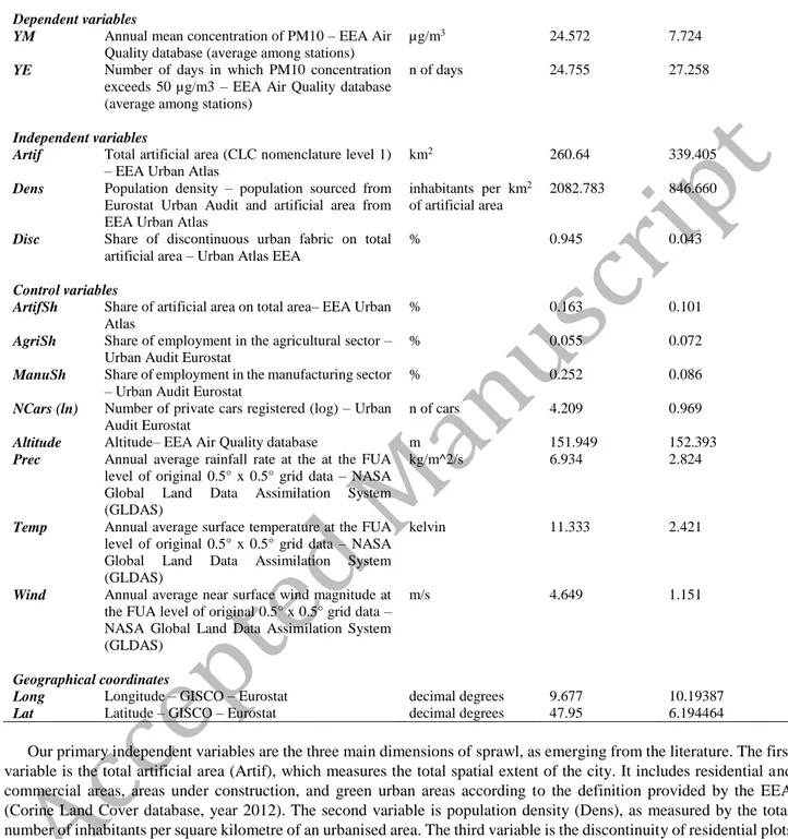
Table 1. Descriptive statistics – Means and Standard Deviations of the variables.

Variable Description of the variable Measure Mean SD

Dependent variables

YM Annual mean concentration of PM10 – EEA Air Quality database (average among stations)

µg/m3 _24.572 _7.724

YE Number of days in which PM10 concentration exceeds 50 µg/m3 – EEA Air Quality database (average among stations)

n of days 24.755 27.258

Independent variables

Artif Total artificial area (CLC nomenclature level 1) – EEA Urban Atlas

km2 _260.64 _339.405

Dens Population density – population sourced from Eurostat Urban Audit and artificial area from EEA Urban Atlas

inhabitants per km2

of artificial area

2082.783 846.660

Disc Share of discontinuous urban fabric on total artificial area – Urban Atlas EEA

% 0.945 0.043

Control variables

ArtifSh Share of artificial area on total area– EEA Urban Atlas

% 0.163 0.101

AgriSh Share of employment in the agricultural sector – Urban Audit Eurostat

% 0.055 0.072

ManuSh Share of employment in the manufacturing sector – Urban Audit Eurostat

% 0.252 0.086

NCars (ln) Number of private cars registered (log) – Urban Audit Eurostat

n of cars 4.209 0.969

Altitude Altitude– EEA Air Quality database m 151.949 152.393

Prec Annual average rainfall rate at the at the FUA level of original 0.5° x 0.5° grid data – NASA Global Land Data Assimilation System (GLDAS)

kg/m^2/s 6.934 2.824

Temp Annual average surface temperature at the FUA

level of original 0.5° x 0.5° grid data – NASA Global Land Data Assimilation System (GLDAS)

kelvin 11.333 2.421

Wind Annual average near surface wind magnitude at

the FUA level of original 0.5° x 0.5° grid data – NASA Global Land Data Assimilation System (GLDAS)

m/s 4.649 1.151

Geographical coordinates

Long Longitude – GISCO – Eurostat decimal degrees 9.677 10.19387

Lat Latitude – GISCO – Eurostat decimal degrees 47.95 6.194464

Our primary independent variables are the three main dimensions of sprawl, as emerging from the literature. The first variable is the total artificial area (Artif), which measures the total spatial extent of the city. It includes residential and commercial areas, areas under construction, and green urban areas according to the definition provided by the EEA (Corine Land Cover database, year 2012). The second variable is population density (Dens), as measured by the total number of inhabitants per square kilometre of an urbanised area. The third variable is the discontinuity of residential plots (Disc), computed as the ratio between the percentage of discontinuous residential area and total residential area. Both variables are sourced from the Corine Land Cover database: the numerator corresponds to the sum of plot areas classified with the code “112 - discontinuous urban fabric”, and the denominator is the sum of plot areas classified with the code “11 – urban fabric”.

We also include several control variables in the regression, accounting for the main sources of PM10 concentrations. Karagulian et al. (2015) identify vehicle traffic, combustions and agriculture, industrial activities, domestic fuel burning, natural sources and unspecified sources of human origin as the main sources of PM10 and PM2.5, globally. Car-dependency, the prevalent use of cars for daily trips to work and for leisure purposes, is partly the consequence of urban morphology (García-Palomares, 2010). Small, dispersed and discontinuous urban environments make the provision of urban transportation infrastructure less viable: the small size of the city does not allow for economies of scale, and the dispersed and discontinuous form requires huge network investments to reach the users. However, car-dependency is also

(7)

7

a result of a household’s behaviour, which is influenced by the socio-economic and cultural context. Including the (log of the) number of registered cars (NCars) in the regression allows to isolate the effects on air pollution of urban forms that require longer and more frequent commuting (which is less feasible using public transportation) from those caused by the use of automobiles that reflects preferences and socio-cultural norms. Moreover, we control for the composition of the economic activity in the city by including the employment shares in the agricultural (Agri_Sh) and manufacturing sectors (Manu_Sh). Further, we include the share of artificial area (Artif_Sh) as a measure of the degree of urbanisation, to which the sources of pollution are connected independently of the specific urban form (compact, dispersed, fragmented). The variable is an important control to isolate the effect of urban form on air quality from other causes of poor air quality not related to the characteristics of urban morphology. Unfortunately, some information is not available for selected cities that are consequently dropped from final database used for the estimation of model parameters. The final sample includes 348 observations.

In addition to these controls, we consider meteorological aspects that may influence air pollution and the geographical position of the region. These are the average temperature measured at the surface, the precipitation rate considering liquid precipitation only, and the average wind speed (Giri et al., 2008; Yi et al., 2010). Higher temperatures are associated with higher mean concentration and a higher probability that the concentration exceeds safeguard limits. More abundant precipitation is expected to lower mean concentration and the probability of exceedance. The effect of wind is controversial. On the one hand, wind helps dissolve particulate matter in the air that otherwise remains trapped on the ground. On the other hand, it brings particulate matter from pollution sources to other places, including cities. The final effect is city-specific, depending on the wind direction and the location of the city with respect to the pollution sources. Hence, it is impossible to disentangle these effects when modelling the average city, as we do in this study. All the meteorological values are sourced from the NASA Global Land Data Assimilation System (GLDAS). The original files are provided in 0.5°x0.5° grid point estimates and aggregated at the city level as the average of all point estimates within the city’s geometry.

We consider the altitude of the city, which is provided as part of the AirQuality EEA database, and expect it to negatively affect the dependent variable. It can have a negative impact on PM10 concentration because pollutants tend to be trapped on the ground, especially under certain meteorological conditions.

Finally, we consider the geographical position of the city by including in the modelling framework the spatial coordinates (latitude and longitude) among the covariates.

3.2 The empirical model

To understand how urban sprawl affects air pollution we estimate different cross-city econometric models. We begin from the simple linear model in equation (1) in which we relate the dependent variable (Y), measured as either the mean concentration level (YM_{) or the number of days in exceedance (Y}E_{) to the three dimensions we use to measure urban}

sprawl, namely, ARTIF, DENS, and DISC. In the latter case, the log-transformation of the dependent variable is applied to correct the excess skewness of the distribution due to the high values on the right tails.

1 2DIS 3 '

Y  ARTIF CDENS X (1)

In equation (1), X is a matrix with all the control variables without the geographical coordinates. According to our research hypothesis that air pollution is higher in larger, more discontinuous and less dense cities, we expect  ₁ 0,

2 0

  , and  ₃ 0.

Geographical coordinates are introduced in equation (2) through a penalised thin plate smooth function s

 

 to capture the trend surface and add smooth spatial structure from the residuals to the fit.

1 2 3 ' ( , )

Y  ARTIF DISCDENS Xs long lat  (2)

The smooth function s(long,lat), or “spatial trend” using a parallel with time series, allows the expected value of Y at one point in space to be conditional on the geographical location of the observation, expressed by longitude and latitude, by considering their interaction (Wood, 2017). The spatial trend surface captures systematic variations of the phenomenon concerned over a region based on geographical locations. Differently from spatial econometrics approaches, where a connectivity or adjacency matrix captures the spatial dimension of the data, the observations’ longitude and latitude are included directly as inputs in the model without considering the relationship with neighbouring observations. The smooth

(8)

8

function reflects the fact that the outcome is not a linear function of either longitude or latitude but rather is an unknown function of both and their interaction and the functional form are estimated non-parametrically1_.

More specifically, the model is estimated via Penalized Iteratively Re-weighted Least Squares: an iterative algorithm selects the smoothing degree (and, hence, the shape of the non-linear function) weighting the explanatory power of the smooth terms on the one hand and the excessive complexity of the functional form on the other through the Generalised Cross Validation criterion. Equation (2) is a GAM and represents the core structure of the empirical approach of this research2_{. The advantage of additive over linear models is the possibility of accounting for and easily estimating}

non-linear relationships. The non-non-linearity can be either expressed as a function of one variable, as in the case of polynomial functions, or as function of more variables, as in the case of interaction terms, to use a parallel with generalised linear models.

To account for these complex non-linear relationships between urban sprawl and air pollution, we also introduce smooth functions to the sprawl variables in two different ways. In the first, we introduce the smooth functions separately. This approach leads to equation (3), from which we can test whether the effect of each characteristic of sprawl on air pollution is non linear. In the second, in equation (4), we introduce a smooth function of density alone and a smooth function of artificial area and discontinuity combined to test the hypothesis that the impact of discontinuity is conditional on the total artificial area.













1 2 3 ' ( , )

Y s ARTIF s DISC s DENS  X s long lat  (3)









12 , 3 ' ( , )

Y s ARTIF DISC s DENS  Xs long lat  (4)

In terms of model structure, GAMs are equivalent to generalised linear models with whom they share the families of models and the link functions for the conditional expectations. Accordingly, the same assumptions of generalised linear models apply. In our case, we assume the normal distribution for both the mean concentration and the number of days in exceedance and, accordingly, the only assumption made for the purpose of estimation is the residuals’ normality.

4. Main Results

4.1 Presentation of results

Table 2 summarises the empirical results. In the first two columns (models (a) and (b) – corresponding to equation (1)), we report the estimates of the linear regression of the annual mean PM10 concentration (a) and days in exceedance (b). Both models return the expected results concerning the effects of urban sprawl on air quality. The coefficients are always significant at the 5% level except for Dens in model (a) that is significant at only 10%. The spatial expansion of cities affects positively PM10 concentration. An increase in the total artificial area of the amount of one standard deviation, approximately 340 km2, corresponds to an increase in the mean concentration of 340*0.0034=1.156 µg/m3 and a 340*0.0005=17% increase in the number of days with emissions exceeding the threshold, other aspects being equal.

1_{For further details about the algebraic formulation of the smooth function refer to Hastie, T. and R. Tibshirani}

(1986,1990) and, for a general introduction, to Wood (2017, Ch 3).

2_{The mgcv R package by Simon Wood has been used for estimation. We estimated all the models with the gam function}

(9)

9

Table 2. PM10 concentration determinants in EU cities, 2014

Linear Additive mean concentration (a) log days in exceedance (b) log days in exceedance (c) log days in exceedance (d) log days in exceedance (e) Intercept 43.9200*** _5.7690*** _1.0780 _1.9030*** _2.0167*** (7.8760) (1.2000) (0.8700) (0.5682) (0.5751) Artif 0.0034*** _0.0005*** _0.0002*** (0.0009) (0.0001) (0.0001) Dens -0.0010* _-0.0002** _-0.0001** (0.0005) (0.0001) (0.0001) Disc -24.6500*** _-2.6080** _0.9930 (7.9080) (1.2050) (0.6308) ArtifSh 1.9300 1.0620 0.2439 0.2741 0.2438 (5.1620) (0.7885) (0.5988) (0.6097) (0.6211) AgriSh 55.9200*** _5.0830*** _1.6460*** _1.3796*** _0.9592** (4.5520) (0.6976) (0.4230) (0.4281) (0.4668) ManuSh 24.7700*** _4.1070*** _0.4314 _0.5957 _0.3979 (3.8700) (0.5902) (0.4323) (0.4417) (0.4817) log(NCars) 1.4100** _0.1566* _0.3065*** _0.3003*** _0.3479*** (0.6160) (0.0953) (0.0622) (0.0661) (0.0729) Altitude -0.0085*** _-0.0015*** _-0.0015*** _-0.0016*** _-0.0017*** (0.0021) (0.0003) (0.0003) (0.0003) (0.0004) Prec -0.1503 -0.0446** _0.0112 _0.0119 _0.0113 (0.1166) (0.0178) (0.0151) (0.0150) (0.0144) Temp -0.1297 -0.0469** _-0.0043 _-0.0069 _-0.0155 (0.1354) (0.0206) (0.0253) (0.0251) (0.0249) Wind -1.4360*** _-0.2967*** _-0.0637 _-0.0936 _-0.1224* (0.3142) (0.0481) (0.0760) (0.0751) (0.0726) Additive terms s(Artif) 2.8330 [0.0195] s(Dens) 3.5120 4.7880 [0.0306] [0.0000] s(Disc) 1.3980 [0.3800] s(Artif,Disc) 2.3810 [0.0000] s(Long,Lat) 8.889 8.7820 9.1460 [0.000] [0.0000] [0.0000] Adj R2 _0.53 _0.43 _0.74 _0.74 _0.76 Dev Explained % 76.1 76.7 79.3

Note to table: standard errors in parenthesis. ***_,**_{, and}*_{indicate significance at the 1%, 5%, and 10% levels, respectively. For the}

additive terms, the values of the F statistics are reported in the table with the relative p-value reported in square brackets. The deviance explained is computed following Wood (2017).

As expected, the effect of density is negative. A decrease in density by the amount of its standard deviation (approximately 850 inhabitants per km2) is associated with an increase in the mean concentration of 850*0.001=0.85 µg/m3 and a 850*0.0002=17% increase in the number of days in exceedance. The use of population density in empirical modelling is instrumental in capturing the increased demand for miles travelled caused by the longer average distance commuted in a low-density built environment. In addition, the average density captures the diversity in transport modes as public transportation services are likely provided less (or less efficiently or altogether not provided) in low-density areas, which encourages the use of private transportation. Longer commutes and higher car dependency as well as more frequent daily trips to access primary services are also expected in fragmented areas, which are favoured by the spatial mismatch between the location of residential plots and that of daily basic services.

In this first specification the effect of urban discontinuity is also negative. An increase in the share of the discontinuous urban fabric equal to its standard deviation, approximately 4%, corresponds to a decrease in the mean concentration of 1.05 µg/m3 and an 11% decrease in the number of days in exceedance.

(10)

10

All the control variables’ coefficients are statistically significant in the model with the number of days as the response variable (b) while only precipitation and temperature coefficients are not significant in the model which explains the average concentration (a). Only the coefficient of the share of artificial area is not statistically significant. Overall, increasing shares of agriculture and manufacturing contribute to increasing air pollution in both models. Worsening air quality is also the result of the high use of cars as a transport vehicle. Finally, bad air quality is negatively associated with the city’s altitude, the average precipitation rate, the average temperature, the average wind speed in the city.

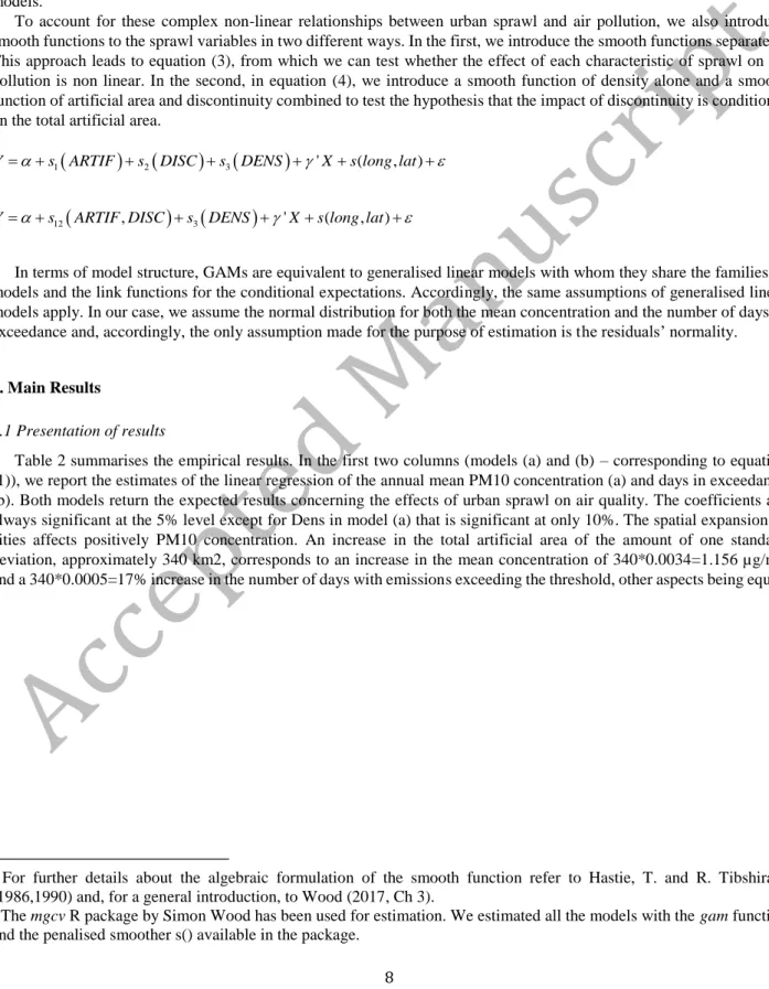
Specifications (a) and (b) returned internally consistent results and evidence that is coherent with the existing empirical studies concerning the role of city size and density, confirming that urban sprawl affects the mean concentration of pollutants as well as the probability of having dangerously high values of concentrations in a large number of days in the year. Nonetheless, both the models show specification problems related to missing factors that explain air pollution. The issue becomes clear by reviewing the spatial distribution of the residuals, which is similar in both models. Figure 1 plots the value of the residuals computed based on the estimates of model (b). Cities with high levels of unexplained numbers of days in exceedance are geographically concentrated in Eastern Germany and Southern Poland, in Romania, and in Northern France and the Benelux area. Particularly high values are visible close to Germany’s border with Denmark. The spatial concentration of high/low values of the residuals in neighbouring cities violates the independence assumption of the linear model, invalidating the estimates.

Figure 1: Spatial distribution of linear model residuals.

Note to figure: The figure plots the city-level map of the residuals of the linear model with the log of the exceedance days as dependent variable. The values are presented using a colour grade scale from green (low value) to red (high values).

The model in equation (2) solves this issue by introducing geographical coordinates into the model via a penalised smooth function, and the results of the GAM are summarised in the third column (c). The smooth function of the geographical coordinates represents a spatial trend that can account for the geographical concentration of the unobserved factors. The previous evidence concerning the role of the artificial area and density holds even after including the spatial trend whereas the counterintuitive result about discontinuity disappears as the coefficient here becomes correctly sloped but statistically insignificant. With the inclusion of the spatial trend, all the control variables retain their sign and

(11)

11

significance, except for the meteorological variables, whose coefficients becomes not statistically significant. The significance of the spatial trend is assessed with standard ANOVA tests in the lower part of the table. In correspondence with the value of s(·) the value of the F statistic of a test comparing the additive model and the same model but without the specific additive component is reported. In the case of the spatial trend, the test compares the model with the trend (c) and the model without (b), and the p-value (reported in square brackets) suggests rejecting the null hypothesis that the geographical position of the city does not affect its pollutant exceedance.

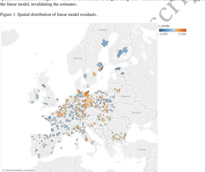
The estimated value of the spatial trend is presented in Figure 2: the figure shows, for each pair of coordinates, the component effect of each of the smooth term model, which adds up to the overall prediction. In the case of geographical coordinates, the figure appears as a set of level curves, each level representing the value of the smooth term: the higher the value of the smooth term (the trend), the higher is the level of the curve. We used a band with graded colours from green (low) to red (high) to indicate the estimated contribution of the geographical position to air pollution. The spatial trend well captures the spatial concentration of high levels of pollution in northern Italy, Germany, and Poland, which also extends to Romania. As a result of the improved capacity of this specification to explain the variation in air pollution levels, the R2 of the model increases compared to the previous models from 0.43 to 0.74, which is a substantial increase, considering that the gain is obtained by adding only two variables .

Figure 2. Location and air pollution – plot of the smooth function of geographical coordinates from the estimates in model (c) in Table 2.

Note to figure: The figure plots the expected values of days in exceedance conditional on the geographical position of the city, as expressed by latitude (Lat) and longitude (Long). The values are presented using a colour grade scale from green (low value) to red (high values).

(12)

12

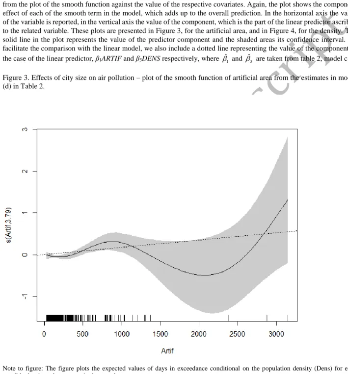
In model (d), we extend the use of penalised smooth functions to the urban sprawl variables using the specification in equation (3). The coefficient estimates of the linear part of the deterministic component of the model; hence, the control variables and the meteorological variables are consistent with the results of the other models, from which they retain sign and significance. Instead, the additive part offers significant insights into the relationship between urban sprawl and air pollution that has not been previously captured. First, there is no evidence of the effect of discontinuity on air pollution, as it is not possible to reject the null hypothesis that the smooth function of discontinuity can be excluded from the model according to the F statistic (p-value = 0.38). Second, it is confirmed that both the spatial size of the city and the average density have an impact on PM10 concentration; however, their effect is largely non-linear. This last evidence emerges from the plot of the smooth function against the value of the respective covariates. Again, the plot shows the component effect of each of the smooth term in the model, which adds up to the overall prediction. In the horizontal axis the value of the variable is reported, in the vertical axis the value of the component, which is the part of the linear predictor ascribed to the related variable. These plots are presented in Figure 3, for the artificial area, and in Figure 4, for the density. The solid line in the plot represents the value of the predictor component and the shaded areas its confidence interval. To facilitate the comparison with the linear model, we also include a dotted line representing the value of the component in the case of the linear predictor, β1ARTIF and β3DENS respectively, where ˆ₁ and ˆ₃ are taken from table 2, model c.

Figure 3. Effects of city size on air pollution – plot of the smooth function of artificial area from the estimates in model (d) in Table 2.

Note to figure: The figure plots the expected values of days in exceedance conditional on the population density (Dens) for each possible density value present in the sample.

In Figure 3, the relationship looks very similar to a polynomial function of the fourth degree. Nonetheless, excluding the three largest cities (with artificial area greater than 1500 km2), the function looks like an inverted U. In the cities below the approximate threshold of 800 km2, for example, Torino, Odense, Antwerpen, Nantes, Hannover, Ostrava, Glasgow, or Helsinki, a spatial expansion will result in increased air pollution. Beyond that threshold, instead, further spatial expansion leads to improvement in the air quality. We tentatively link this evidence to the presence of scale effects

(13)

13

in the provision of public services, which contribute substantially to reducing PM10 concentration. In small cities, the provision of public transportation services is not economically viable because the scale of the city and the potential demand do not justify an expansion of the network to allow full provision of service. Thus, an expansion of the city likely translates into longer and more frequent car-based trips. In contrast, in large cities, the economies of scale make the provision of public transportation affordable; the larger the scale, the more efficient this provision is, allowing car-based trips to be limited and air pollution to be contained.

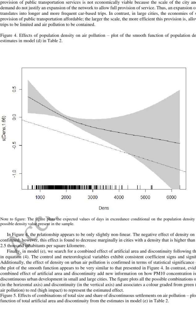
Figure 4. Effects of population density on air pollution – plot of the smooth function of population density from the estimates in model (d) in Table 2.

Note to figure: The figure plots the expected values of days in exceedance conditional on the population density (Dens) for each possible density value present in the sample.

In Figure 4, the relationship appears to be only slightly non-linear. The negative effect of density on air pollution is confirmed; however, this effect is found to decrease marginally in cities with a density that is higher than approximately 2.5 thousand inhabitants per square kilometre.

Finally, in model (e), we search for a combined effect of artificial area and discontinuity following the specification in equation (4). The control and meteorological variables exhibit consistent coefficient signs and significance values. Additionally, the effect of density on urban air pollution is confirmed in terms of statistical significance (p<0.001), and the plot of the smooth function appears to be very similar to that presented in Figure 4. In contrast, evidence about the combined effect of artificial area and discontinuity add new information on how PM10 concentration is influenced by discontinuous urban development in small and large cities. The figure plots all the possible combinations of artificial area (in the horizontal axis) and discontinuity (in the vertical axis) and associates a colour graded from green (low impact on air pollution) to red (high impact) to represent the estimated effect.

Figure 5. Effects of combinations of total size and share of discontinuous settlements on air pollution – plot of the smooth function of total artificial area and discontinuity from the estimates in model (e) in Table 2.

(14)

14

Note to figure: The figure plots the expected values of days in exceedance conditional on the levels of artificial area (Artif) and settlement discontinuity (Disc) for each possible combination of Artif and Disc present in the sample. The values are presented using a colour grade scale from green (low value) to red (high values).

The largest effect on air pollution is generated by the combination of high artificial area and high discontinuity, the upper right part of Figure 5. Indeed, as emphasised by Dupont (2007), peri-urban planning is non-neutral from a political perspective. Polluting and heavy industries usually tend to be relocated in the peripheries of large cities so as to reduce pollution in the city centre. In contrast, discontinuity does not contribute to worsening air pollution in small cities (Artif<500 Km2) as the estimated effect on air quality remains low (the green area in the left part of the figure) independently on the level of discontinuity.

4.2 Discussion

The empirical results presented are consistent with the findings of previous empirical analysis about the relationship between air quality and urban form. As anticipated in the introduction, most of the literature focused on CO2 emissions rather than air pollution to understand the impact of urban form and, hence, the results of the empirical analysis are not directly comparable. Nonetheless, we found interesting parallels.

A significant impact of artificial area on air quality is found in Bart (2010), Cirilli and Veneri (2014), McCarty and Kaza (2015), and Cárdenas Rodríguez et al. (2016). Such evidence suggests that air pollution, either measured as CO2 emission or pollutant concentration, linearly increases with the size of cities. We find a similar result as well, with a linear coefficient associated to artificial area positive and statistically significant in both the regressions of mean concentration and days in exceedance (table 2, models a and b). We show, however, that such linear relationship masks a more complex

(15)

15

inverse U patterns: urban area growth impacts positively air pollution in small (Km2<800) cities, then the impact turns negative in medium size cities (1500>Km2>800) to become positive again in large metropolitan areas (Km2>1500).

Concerning density, all the existing studies converge to the same result: air pollution increases when the density of a city decreases. Cirilli and Veneri report a negative coefficient for density in the CO2 emission per passenger regression. McCarty and Kaza (2015) find the geographical concentration of high density counties to affect negatively the exceedances, in particular Ozone exceedances. Cárdenas Rodríguez et al. (2016), in contrast, find a positive association between density and SO2 concentration and a lack of explanatory power of density in the regression of PM and NO2. The result may look in contrast to other existing evidence. It is worth noting, however, that coal fired power stations rather than traffic is the main source of NO2, and the link with density may reflect the location of power plants in the proximity of urban areas in specific regions of Europe where coal is a relevant source of energy production, like Poland. Compared to the existing literature, our result confirms that that higher densities are associated to lower concentrations of pollutants and, hence, a better air quality. Oppositely to the case of total urbanised area, we do not find strong evidence of non-linearity in the effect of density (other than those captured by the log-transformation of the dependent variable).

The most interesting result concerns the fragmentation of urbanised area, also defined as spatial discontinuity of urbanisation. McCarty and Kaza (2015) use several indicators of spatial discontinuity and find that exceedances increase with the increase in the number of patches, the decrease in the mean urban patch size, and the increase of its standard deviation. When the analysis focuses on PM, however, only the number of patches shows a significant relationship with air quality. The effect of the number of fragments is also found positive in Cárdenas Rodríguez et al. (2016), even though weakly significant (0.05<p<0.1) in the analysis of PM. In our study, the estimated coefficient on fragmentation is statistically significant but negative. It turns insignificant when the spatial trend is added to the model and becomes significant again when considered alongside total urbanised area. The overall effect is positive for large urban areas only, accordingly, meaning than an increase in discontinuity (equivalent to an increase in the number of patches or fragments in the other studies) has a positive effect on the number of exceedances.

In summary, the evidence suggests that the spatial expansion of cities per se is not the cause of the deteriorating air quality, at least in medium size cities. Density has a clear effect but most of the problems related to the urban form involve primarily large cities and metropolitan areas, at least when the spatial expansion comes in tandem with an increase in discontinuity and generates leapfrog urban development. Based on these evidences, we confirm that the development of new suburban employment clusters within the boundaries of metropolitan areas as an important factor inducing the spatial expansion of cities Felstenstein (2002). This has important consequences in terms of air pollution: a first effect is certainly given by emissions generated by additional industrial activities, which is confirmed in our results by the positive effect brought about by the share of manufacturing. Further, new suburban employment clusters allegedly attract workers to reside in their proximity which, in their turn, demand for the presence of retail and entertainment in the vicinity, thus resulting in higher land conversion (Herzog and Schlottman 1991; Malecki and Bradbury 1992) and domestic fuel consumption.

5. Conclusion

The extent to which integrated transport and planning policies can effectively mitigate the pollution of air remains an open question for policymakers and especially urban planners. Intuitively, more compact urban forms that require a lower dependency on private transportation should benefit air quality. The existing research has focused on the effect of compact urban form to investigate this link, and the results demonstrate that a lower PM10 concentration can be associated with a more compact urban structure. Despite this clear evidence, urban structures continue to evolve in the direction of low-density urban development on the peripheries that are also increasingly becoming characterised by a spatial discontinuity of the built-up area, especially residential settlements.

In this paper, we document the overall negative effects of urban sprawl, considered in its multiple dimensions of low-density and high-discontinuity urban development on the annual average PM10 concentration and the number of days in which PM10 concentration exceeds the safeguard threshold for citizens in EU cities. The empirical analysis contributes to the existing literature about urban sprawl and air quality considering the different characteristics of urban sprawl and their interaction. The evidence shows that these negative effects come from both low-density urbanisation and high spatial discontinuity; however, the latter effect is evidenced only in highly urbanised contexts, likely large cities. The results of the paper are robust to the inclusion of controls for city-specific characteristics, climatic conditions and unobservable characteristics related to the geographical location of the city.

For many years, urban sprawl has remained an ignored challenge. Emotional sentiments in favour of or against the spatial expansion of built-up areas and the sealing of soil have mainly driven the debate about urban sprawl, which has additionally been fuelled by disagreements about measures of sprawl. As a result, the discussion about the potential environmental consequences of sprawl is confined within the boundary of the comparison between the compact model of

(16)

16

urban growth and its possible alternative. Most of the recent streams of research on urban sprawl shed light on the multiple dimensions of urban sprawl. Low-density but also a high discontinuity of residential settlements led by changing household preferences and the diffusion of cars are shaping the urban form of modern cities, especially the largest ones. Documenting the environmental damage coming from the combination of these factors should raise awareness of the consequences of the current trends in urban development in Europe and prevent urban sprawl from continuing to be an ignored challenge. At the same time, the evidence in this paper relates pollution concentration to some specific characters of urban sprawl, indicating that the effect is highly context- and location-specific and caution is needed when translating this evidence into a policy message.

While air quality remains one of the many indicators of the quality of the urban environment and, consequently, of citizen’s health that can be affected by urban sprawl, it is a critical one, and more research and evidence is needed to adequately assess the impact of urban sprawl on our lives.

(17)

17

References

Arribas-Bel, D., Nijkamp, P., & Scholten, H. (2011). Multidimensional urban sprawl in Europe: a self-organizing map approach. Computers, Environment and Urban Systems, 35(4), 263–275.

Bandeira, J.M., Coelho, M.C., Sá, M.E., Tavares, R., & Borrego, C. (2011). Impact of land use on urban mobility patterns, emissions and air quality in a Portuguese medium-sized city. Science of The Total Environment, 409(6), 1154–1163. Barla, P., Miranda-Moreno, L.F., & Lee-Gosselin, M. (2011). Urban travel CO2 emissions and land use: a case study for

Quebec City. Transportation Research Part D: Transport and Environment, 16(6), 423–428.

Bart, I.L. (2010). Urban sprawl and climate change: a statistical exploration of cause and effect, with policy options for the EU. Land Use Policy, 27(2), 283–292.

Borrego, C., Martins, H., Tchepel, O., Salmim, L., Monteiro, A., & Miranda, A.I. (2006). How urban structure can affect city sustainability from an air quality perspective. Environmental Modelling & Software, 21(4), 461–467.

Brueckner, J.K. (2000). Urban sprawl: diagnosis and remedies. International Regional Science Review, 23(2), 160–171. Brueckner, J.K., & Fansler, D.A. (1983). The economics of urban sprawl: theory and evidence on the spatial sizes of

cities. The Review of Economics and Statistics, 65(3), 479–482.

Cárdenas Rodríguez, M., Dupont-Courtade, L., & Oueslati, W. (2016). Air pollution and urban structure linkages: evidence from European cities. Renewable and Sustainable Energy Reviews, 53, 1–9.

Cho, H.-S., & Choi, M.J. (2014). Effects of compact urban development on air pollution: empirical evidence from Korea. Sustainability, 6(9), 5968–5982.

Cirilli, A., & Veneri, P. (2014). Spatial structure and carbon dioxide (CO2) emissions due to commuting: an analysis of Italian urban areas. Regional Studies, 48(12), 1993–2005.

Coker, E.S., Cavalli, L., Fabrizi, E., Guastella, G., Lippo, E., Parisi, M.L., Pontarollo, N., Rizzati, M., Varacca, M., & Vergalli, S. (2020). The effects of air pollution on COVID-19 related mortality in Northern Italy. Environmental and Resource Economics, 76, 611–634.

Cole, M.A., Ozgen, C. & Strobl, E. Air pollution exposure and Covid-19 in Dutch municipalities. Environmental and Resource Economics, 76, 581–610 (2020).

Conticini E, Frediani B, Caro D (2020) Can atmospheric pollution be considered a co-factor in extremely high level of SARS-CoV-2 lethality in Northern Italy? Environmental Pollution, 261:114465

Daniels, B., Zaunbrecher, B.S., Paas, B., Ottermanns, R., Ziefle, M., & Roß-Nickoll, M. (2018). Assessment of urban green space structures and their quality from a multidimensional perspective. Science of the Total Environment, 615, 1364–1378.

Dupont, V. (2007). Conflicting stakes and governance in the peripheries of large Indian metropolises–An introduction. Cities, 24(2), 89–94.

DuPont, A. (2018). Improving and monitoring air quality. Environmental Science and Pollution Research, 25(15), 15253-15263.

EEA-FOEN (2016). Urban sprawl in Europe. EEA Report No 11/2016. European Environment Agency.

European Environment Agency (2017). European Union emission inventory report 1990-2015 under the UNECE Convention on Long-range Transboundary Air Pollution (LRTAP). European Environment Agency.

European Environment Agency (2019). Air quality in Europe - 2018 report. EEA Report No 12/2018, European Environment Agency.

Ewing R.H. (2008). Characteristics, causes, and effects of sprawl: a literature review. In Marzluff, J.M., Shulenberger, E., Endlicher, W., Alberti, M., Bradley, G., Ryan, C., Simon, U. & ZumBrunnen, C. (Eds). Urban Ecology. Boston, MA, Springer.

Felsenstein, D. (2002). Do high technology agglomerations encourage urban sprawl?. The Annals of Regional Science, 36(4), 663–682.

Ferreira, F., Gomes, P., Tente, H., Carvalho, A.C., Pereira, P., & Monjardino, J. (2015). Air quality improvements following implementation of Lisbon’s Low Emission Zone. Atmospheric Environment, 122, 373–381.

Frank, L.D., Stone, B., & Bachman, W. (2000). Linking land use with household vehicle emissions in the central puget sound: methodological framework and findings. Transportation Research Part D: Transport and Environment, 5(3), 173–196.

Frenkel, A., & Ashkenazi, M. (2008). Measuring urban sprawl: how can we deal with it?. Environment and Planning B: Planning and Design, 35(1), 56–79.

Galster, G., Hanson, R., Ratcliffe, M. R., Wolman, H., Coleman, S., & Freihage, J. (2001). Wrestling sprawl to the ground: defining and measuring an elusive concept. Housing policy debate, 12(4), 681–717.

García-Palomares, J.C. (2010). Urban sprawl and travel to work: the case of the metropolitan area of Madrid. Journal of Transport Geography, 18(2), 197–213.

Giri, D., Krishna Murthy, V., & Adhikary, P.R. (2008). The influence of meteorological conditions on PM10 concentrations in Kathmandu Valley. International Journal of Environmental Research, 2(1), 49–60.

(18)

18

Glaeser, E.L., & Kahn, M.E. (2004). Sprawl and urban growth. In Vernon Henderson, J., & Thisse, J.F. (Eds.). Handbook of Regional and Urban Economics. Elsevier, Volume 4, 2481–2527.

Guastella, G., Oueslati, W., & Pareglio, S. (2019). Patterns of urban spatial expansion in European cities. Sustainability, 11(8), 2247.

Guo, Y., Su, J.G., Dong, Y., & Wolch, J. (2019). Application of land use regression techniques for urban greening: an analysis of Tianjin, China. Urban Forestry & Urban Greening, 38, 11–21.

Hastie, T., & Tibshirani, R. (1986). Generalized additive models (with discussion). Statistical Science, 1, 297–318. Hastie, T., & Tibshirani, R. (1990). Generalized Additive Models. London, Chapman & Hall.

Herzog, H.W., & Schlottmann, A.W. (1991) Metropolitan dimensions of high technology location in the U.S.: worker mobility and residential choice. In Herzog, H.W., & Schlottmann, A.M. (Eds.). Industry location and public policy. University of Tennessee Press, Knoxville TN, 169–189

Janhäll, S. (2015). Review on urban vegetation and particle air pollution - Deposition and dispersion. Atmospheric Environment, 105, 130–137.

Janssen, N.A.H., Fischer, P., Marra, M., Ameling, C., & Cassee, F.R. (2013). Short-term effects of PM2.5, PM10 and PM2.5-10 on daily mortality in the Netherlands. Science of the Total Environment, 463–464, 20–26.

Karagulian, F., Belis, C.A., Dora, C.F.C., Prüss-Ustün, A.M., Bonjour, S., Adair-Rohani, H., & Amann, M. (2015). Contributions to cities' ambient particulate matter (PM): A systematic review of local source contributions at global level. Atmospheric Environment, 120, 475-483.

Lee, S., & Lee, B. (2014). The influence of urban form on GHG emissions in the U.S. household sector. Energy Policy, 68, 534–549.

Lelieveld, J., Klingmüller, K., Pozzer, A., Pöschl, U., Fnais, M., Daiber, A., & Münzel, T. (2019). Cardiovascular disease burden from ambient air pollution in Europe reassessed using novel hazard ratio functions. European Heart Journal, 1–7.

Litschike, T., & Kuttler, W. (2008). On the reduction of urban particle concentration by vegetation - A review. Meteorologische Zeitschrift, 17(3), 229–240.

Liu, Q. (2014). Electric car with solar and wind energy may change the environment and economy: a tool for utilizing the renewable energy resource. Earth’s Future, 2(1), 7–13.

Liu, X., & Sweeney, J. (2012). Modelling the impact of urban form on household energy demand and related CO2 emissions in the Greater Dublin Region. Energy Policy, 46(Supplement C), 359–369.

Lu, C., & Liu, Y. (2016). Effects of China’s urban form on urban air quality. Urban Studies, 53(12), 2607–2623. Malecki, E.J., Bradbury, S.L. (1992). R&D facilities and professional labor: labor force dynamics in high technology.

Regional Studies, 26, 123–136

Martins, H., Miranda, A., & Borrego, C. (2012). Urban structure and air quality. In Budi, H. (Ed.). Air pollution: a comprehensive perspective. London, InTech Open.

McCarty, J., & Kaza, N. (2015). Urban form and air quality in the United States. Landscape and Urban Planning, 139, 168–179.

Newman, P., & Kenworthy, J. (2006). Urban design to reduce automobile dependence. Opolis, 2(1), 35–52. OECD (2018). Rethinking urban sprawl: moving towards sustainable cities. Paris, OECD Publishing.

Ogen, Y. (2020). Assessing nitrogen dioxide (NO2) levels as a contributing factor to coronavirus (COVID-19) fatality. Science of the Total Environment, 726, 138605

Pascal, M., Falq, G., Wagner, V., Chatignoux, E., Corso, M., Blanchard, M., Host, S., Pascal, L., & Larrieu, S. (2014). Short-term impacts of particulate matter (PM10, PM10-2.5, PM2.5) on mortality in nine French cities. Atmospheric Environment, 95, 175–184.

Santi, P., Resta, G., Szell, M., Sobolevsky, S., Strogatz, S., & Ratti, C. (2014). Quantifying the benefits of vehicle pooling with shareability networks. Proceedings of the National Academy of Sciences, 111 (37) 13290–13294.

Schwarz, N. (2010). Urban form revisited — Selecting indicators for characterising European cities. Landscape and Urban Planning, 96(1), 29–47.

She, Q., Peng, X., Xu, Q., Long, L., Wei, N., Liu, M., Wenxiao j., Taoye Z., Ji H., & Xiang, W. (2017). Air quality and its response to satellite-derived urban form in the Yangtze River Delta, China. Ecological Indicators, 75, 297–306. Shi Y, Wang Y, Shao C, Huang J, Gan J, Huang X, Bucci E, Piacentini M, Ippolito G, Melino G (2020). COVID-19

infection: the perspectives on immune responses. Cell Death & Differentiation, 27(5), 1451-1454

Sovacool, B.K., & Brown, M.A. (2010). Twelve metropolitan carbon footprints: a preliminary comparative global assessment. Energy Policy, 38(9), 4856–4869.

Stafoggia, M., Zauli-Sajani, S., Pey, J., Samoli, E., Alessandrini, E., Basagaña, X., …, & Forastiere, F. (2015). Desert dust outbreaks in Southern Europe: contribution to daily PM 10 concentrations and short-term associations with mortality and hospital admissions. Environmental Health Perspectives, 124(4), 413–419.

Stone, B., Mednick, A.C., Holloway, T., & Spak, S.N. (2007). Is compact growth good for air quality? Journal of the American Planning Association, 73(4), 404–418.