MODELLING SHOT LENGTHS OF HOLLYWOOD MOTION
PICTURES WITH THE DAGUM DISTRIBUTION
Nick Redfern1
School of Arts and Communications, Leeds Trinity University, Leeds, UK
1. INTRODUCTION
With the application of artificial intelligence to filmmaking, decisions about shot selec-tion, ordering, and duration are progressively moving out of the hands of motion picture editors and are being taken over by computers. In 2016, 20th Century Fox released the trailer for its AI science-fiction horror/thriller Morgan. This trailer was produced by training the IBM supercomputer Watson on a sample of 100 horror film trailers in or-der to identify which moments should be included in the trailer forMorgan. Watson isolated 10 scenes totalling six minutes of video that were then shaped into a final cut by a human editor, thereby reducing the total production time from the 10 to 30 days that is typical for trailer production to 24 hours (Smithet al., 2017). The following year, a paper by researchers at Stanford University and Adobe, makers of the non-linear edit-ing suite Premiere Pro, described an idiomatic editedit-ing system enabledit-ing filmmakers to build custom editing styles by controlling a range of parameters (e.g. the visibility of the speaker, avoiding jump cuts, etc.) that are then applied to a collection of takes of a scene to generate dialogue scenes in a handful of seconds (Leakeet al., 2017). As these examples show, as the role of artificial intelligence in filmmaking grows it will increas-ingly be the case that the decisions of filmmakers will focus on the selection of models for computers to shape the final form of a film. Consequently, a key area in the de-velopment of computational filmmaking technologies is the selection and clarification of those models that can be used to efficiently generate appropriately edited sequences (Ronfard, 2017). A major issue is the identification of statistical distributions that can act as a model for motion picture shot lengths in order to determine shot duration and shape the pacing of a film. Shot duration is a key indicator of film style and has long been used as a low-level visual feature in applied media aesthetics for the automated clas-sification and summarization of video (Álvarezet al., 2019), with a range of distributions considered (Vasconcelos and Lippman, 2000; Taskiran and Delp, 2002). Due to the pos-itively skewed nature of motion picture shot length distributions, a common choice for
automated editing systems is the two-parameter lognormal distribution (Galvaneet al., 2015a,b). While it has a skew to the upper tail the lognormal distribution often does not fit the observed data, with many shot length distributions remaining skewed after application of a logarithmic transformation to shot length data. While the application of a Yeo-Johnson transformation to the log-transformed data has been suggested as a solution to this problem, there are often more shots of shorter duration evident in the lower tail of a shot length distribution than expected once the second transformation is applied (Baxter, 2014).
In this paper, I analyse the use of the three-parameter Dagum distribution for mod-elling shot length distributions in Hollywood motion pictures. As a special case of the four-parameter generalized beta distribution of the second kind, the Dagum distribution has two shape parameters and covers a region of the skewness-kurtosis plane, whereas the lognormal distribution has only a single shape parameter and corresponds to a line in the skewness-kurtosis plane as a special case of the three-parameter lognormal distribu-tion (McDonaldet al., 2013). The flexible shape of the Dagum distribution suggests it as a candidate for shot length distributions capable of modelling a wide range of skewness and kurtosis values and a variety of tail behaviours. I compare the fit of the Dagum dis-tribution and the lognormal disdis-tribution to a sample of 134 Hollywood films released from 1935 to 2005. The advantages of this paper lie in its discussion of the shape of motion picture shot length distributions, which to date has not received the same level attention as the average shot length in analyses of film style. I show how the shape pa-rameters of the Dagum distribution determine the shape of a shot length distribution and make recommendations for selecting parameters for models for four different types of Hollywood films.
2. MODELS OF SHOT LENGTH DISTRIBUTIONS
2.1. The Dagum distribution
The Dagum distribution is a heavy-tailed distribution proposed by Dagum (2008) for modelling income distributions and has also been applied to meteorological, hydrolog-ical, and waiting time data. There are different versions of the Dagum distribution: a three-parameter distribution (Type I) and a four-parameter specification (Type II). Here I focus on the three-parameter Type I Dagum distribution. The Dagum distribution is a special case of the four-parameter generalized beta distribution of the second kind, with shape parameterq equal to 1. It is related to the Burr XII (Singh-Maddala) distribution and is also known as the inverse Burr or Burr III distribution.
The probability density function of the Dagum distribution is
f(x;a, b, p) = a p x b a p x 1+ x b ap+1 ,x> 0,
where p> 0 and a > 0 are shape parameters and b > 0 is a scale parameter. The distri-bution function is F(x;a, b, p) = 1+ x b −a− p .
Kleiber (2008) gives a detailed summary of the properties and functions of the Dagum distribution.
2.2. The lognormal distribution
The two-parameter lognormal distribution is defined in relation to the normal distribu-tion: a random variableX is lognormally distributed if its logarithm (Y = log(X )) is normally distributed. The lognormal distribution is a continuous probability distribu-tion with the density funcdistribu-tion
f(x;µ,σ) = 1 xσp2πexp − 1 2σ2(log x − µ) 2,x> 0,
whereµ is the arithmetic mean and σ is the standard deviation of Y = log(X ). The distribution function is F(x;µ,σ) = 1 σp2π Z∞ 0 1 texp §−(log t − µ)2 2σ2 ª d t .
This distribution is a special case of the three-parameter lognormal distribution with location parameter (γ) equal to 0. Kleiber and Kotz (2003, pp. 107-145) provide a detailed review of the properties and functions of the lognormal distribution.
3. METHODOLOGY
3.1. Data
The data used here comprises 134 Hollywood films released between 1935 and 2005 di-vided into five genres (action, adventure, animation, comedy, and drama) from Cutting et al. (2010), and is available through the Cinemetrics database atwww.cinemtrics.lv/ database.php.
3.2. Parameter estimation
The parameters of both distributions were estimated by maximum likelihood using the R (R Core Team, 2018) packagesfitdistrplus (Delignette-Muller and Dutang, 2015) andactuar (Dutang et al., 2008).
3.2.1. Dagum distribution
Inactuar, the Dagum distribution is called the inverse Burr distribution and is fitted using theinvBurr root function. For a random sample of size n from the Dagum dis-tribution with parameters p, a, and b , the log-likelihood function is
` = n loga + n log p + (a p − 1)Xn i=1 logxi− na p log b − ( p + 1) n X i=1 log 1+ x i b a .
The maximum likelihood estimators of the parameters are obtained numerically by maximizing the log-likelihood function with respect to p, a, and b by solving∂ p∂ ` = 0,
∂ `
∂ a= 0, and∂ b∂ ` = 0. Kleiber (2008, p. 108) gives the likelihood equations for each
param-eter. fitdistrplus::fitdist requires starting values to fit the Dagum distribution, and those used here were shape 1 (p)= 1, shape 2 (a) = 1, and scale (b) = 1. When no result was returned, the starting value for the shape 1 parameter was increased through the sequence 15, 30, and 45 until a fitted distribution was returned.
3.2.2. Lognormal distribution
The log-likelihood function for the 2-parameter lognormal distribution is
` = −n 2log(2πσ 2) −Xn i=1 logxi− Pn i=1logxi2 2σ2 + Pn i=1logxiµ σ2 − nµ2 2σ2
and has a closed-form solution. Maximising` with respect to µ and σ, the maximum likelihood estimators are
ˆ µ = 1 n n X i=1 logxi and c σ2= 1 n n X i=1 (log xi− ˆµ)2. 3.3. Goodness-of-fit
Four methods are used to assess goodness-of-fit of the Dagum and lognormal distribu-tions to shot length data. Numerical goodness-of-fit summaries are produced using the functionfitdistrplus::gofstat(). Due to limitations of space I include only a lim-ited number of examples of individual films here. Full results for all films in the sample is available in the supplementary material for this article.
3.3.1. Cumulative distribution statistics
The Kolmogorov-Smirnov (K-S) statistic is the maximum absolute distance between the empirical CDF (F0(x)) to the distribution function of the model distribution (F (x)):
D= max|F0(x) − F (x)|.
The K-S statistic is sensitive to deviations from the model in the centre of the distribu-tion. The Anderson-Darling (A-D) distance also compares the empirical CDF to the distribution function of the model distribution but is more sensitive to differences in the tails: A2= n Z∞ −∞ (F0(x) − F (x))2 F(x)(1 − F (x))d F(x).
These statistics are used to compare the distance between the Dagum and lognormal models to the shot lengths of each film in the sample, with the model with the smaller distance to the empirical CDF preferred.
3.3.2. Bayesian information criterion
I am comparing the performance of two models with different numbers of parameters, and so I use the Bayesian information criterion (BIC) for model selection:
B I C= −2log(L(Θ)) + k log(n).
The BIC balances model fit, based on the likelihood of the model fitted to the data for the maximum likelihood parameters ofΘ , and complexity, penalising the fit for the sample size (k) and the number of parameters (n). The model with the lower BIC is preferred. Raftery (1995) proposed the following guidelines for interpreting the absolute difference between BICs of two models: a difference between 0 and 2 is weak evidence in favour of a particular model; a difference between 2 and 6 is positive evidence; a difference between 6 and 10 is strong evidence; and a difference greater than 10 is very strong evidence.
3.3.3. Graphical methods
I use three graphical methods for assessing goodness-of-fit. The probability density func-tions of the shot length data and the theoretical quantiles for the lognormal and Dagum distributions fromfitdistrplus::qqcomp() were plotted using ggplot2::geom_line (stat=`density'). CDF plots were produced using the fitdistrplus::cdfcomp() function for comparison of the empirical cumulative distribution function and the dis-tribution functions of the fitted disdis-tributions and to give concrete meaning to the K-S and A-D distances. Quantile-quantile (Q-Q) plots visualise the fit between the observed values and the estimated values of the model distribution: if the data are well fitted by the model, then the points in the plot should lie on the 45-degree line. A Q-Q plot can be used to identify why a theoretical distribution does not fit the data, and can detect
differences in location, scale, asymmetry, deviations in the tails, and outliers. The Q-Q plots were produced using thefitdistrplus::qqcomp() function. An advantage of these plots is that they allow for the visual comparison of both the model distributions assessed here and may reveal which model fits the data best when both are indicated to be good fits according to numerical goodness-of-fit statistics or where there is conflicting evidence between those statistics.
4. RESULTS FORHOLLYWOOD MOTION PICTURES, 1935-2005 4.1. Goodness-of-fit results
Visual inspection of the probability density functions, cumulative distributions func-tions and Q-Q plots for each film show that, overall, shot length data of films in the sample is well-fitted by the three-parameter Dagum distribution. This distribution also fits the better than the two-parameter lognormal distribution, with the latter providing an adequate fit for only a small proportion of films. There are some films for which neither distribution adequately fits the data. Interestingly, this tends to be restricted to some films released in 1945, 1950, and 1960 with films released in other years well-fitted by at least one, if not both, of these distributions.
Comparing the goodness-of-fit statistics for the two theoretical distributions we see that the K-S distance is smaller for the fitted Dagum distribution for 86% of films in the sample, though the differences between this and the fits of the lognormal distribution are typically small. The A-D distances are smaller for the Dagum distribution for 83% of films and with larger differences when compared to the fit of the lognormal distri-bution, indicating the former is better able to fit the tails of shot length distributions. Applying Raftery’s criteria for interpreting differences in BIC, there are four films with an absolute difference less than 2 indicating differences in model fit that are not worth mentioning. Of the remaining 130 films, the BIC for the fitted Dagum distribution is lower for 90 films (69%). When the BIC indicates the Dagum distribution is a better fit, the K-S and A-D distances also indicate this and there are no conflicting numerical goodness-of-fit results. When the BIC is lower for the lognormal distribution there are no conflicts with the CDF-based statistics for 17 films (13%), but at least one of the K-S or A-D distances indicates a better fit for the Dagum distribution for the remaining 23 films. Of the forty films with a BIC difference indicating positive evidence in favour of the lognormal distribution, 29 were released between 1935 and 1970, inclusive, with only 11 released from 1975. This suggests that the lognormal distribution better fits the slower-paced editing style of classical Hollywood cinema (1917-1960) than the more rapid editing characteristic of the intensified continuity style of contemporary Holly-wood filmmaking (Bordwell, 2006). Figure 1 plots the BIC differences for all films in the sample and shows that the animation genre stands out as the one genre for which the majority of films are better fitted by the lognormal distribution.
The superior fit of the Dagum distribution is due to it having two shape parameters that give it its flexible shape, whereas the lognormal distribution, having only a single
Figure 1 – Differences in Bayesian information criterion (BIC) for fitted three-parameter Dagum distribution and two-parameter lognormal distribution for shot length data of 134 Hollywood films released from 1935 to 2005 (Source: Cuttinget al. (2010);http://www.cinemetrics.lv/ database.php). Negative differences indicate the Dagum distribution is the preferred model.
Figure 2 – Probability density function (A), cumulative distribution function (B) and quantile-quantile (C) plots for fitted three-parameter Dagum and two-parameter lognormal distributions forBack to the Future (1985).
shape parameter, cannot be bent enough to fit the data. This can be seen in Figure 2 when fitting the distributions to shot length data forBack to the Future (1985). The shapes of the probability density function (Figure 2.A) and the Q-Q plot (Figure 2.C) show the logarithmic transformation fails to remove the skew of the data. The Dagum distribution typically fits the lower tail better than the lognormal distribution which predicts a much shorter tail than is actually observed, though, as the example ofBack to the Future shows, the lognormal distribution can provide a better fit to the upper tail. The shot length data in the right tail for this film is lighter than that predicted by the Dagum distribution, but as the data is concentrated in the left tail the overall fit is better. The peak of the empirical distribution is greater than that predicted by the lognormal distribution. These are common patterns across the majority of films in the sample.
4.2. The shape of shot length distributions
Skewness (S) and kurtosis (K) describe the shape of a distribution and are, respectively, the third S= E[(x − µ) 3] (E[(x − µ)2])32 = m3 m32 2 and fourth K= E[(x − µ) 4] (E[(x − µ)2])2= m4 m2 2
standardized moments. Skewness measures the symmetry of a distribution based on the relative sizes of the tails. A distribution with tails of equal weight will have a skewness of zero and be symmetric, while distributions with a more massive right(left)-hand tail will have a positive(negative) skewness value. Kurtosis is a measure of the combined weight of the tails relative to the rest of a distribution, with higher values of kurtosis indicating heavier tails. Kurtosis doesnot describe the peakedness of a distribution (Westfall, 2014). Beyond noting they are positively skewed, little attention has been paid to the shape of shot length distributions. Kohara and Niimi (2013) compared the shape of the distri-butions of films by three Japanese animation directors, interpreting differences in skew-ness as evidence of the distinctive shot length styles of the directors. However, their dis-cussion of the kurtosis of shot length distributions was incorrectly presented in terms of the peakedness of the distributions and not the relative weight of the tails. Baxter (2014) looked at the skewness and (excess) kurtosis values of log-transformed shot length dis-tributions to assess departures from lognormality, finding that applying a logarithmic transformation did not remove the skewness from the data and that films released after 1975 tended to have higher kurtosis values than films released before that date. Baxter subsequently applied a Yeo-Johnson transformation to log-transformed shot length data in order to ‘normalise’ the data, finding that films released after 1975 deviate from the ‘normal’ distribution with more shorter shot lengths than expected often showing in the lower tail of the distributions.
Figure 3 plots the skewness and kurtosis values of the films in the sample. In the skewness-kurtosis plane the observations for the films in the sample all lie in the Dagum region between the lower bound for the Dagum distribution and the curve correspond-ing to feasibleS-K combinations for the lognormal distribution. The generalised Gamma distribution which also covers the region between the lower bound of the Dagum dis-tribution and the lognormal curve does not appear to be a good fit for Hollywood films but may perform better for films with a slower editing style. Films better fitted by the lognormal distribution tend to have lower values of skewness and kurtosis among the sample (S< 4 and K < 15), but in general the lognormal distribution tends to underesti-mate the skewness and overestiunderesti-mate the kurtosis of the data resulting in the poorer fit we see in Figure 2 and for many films in the sample. There are no differences in values for S and K among the five genres, but there is a clear tendency for films in the sample with release dates after 1975 to exhibit both greater skewness and kurtosis values than films in the sample released before that date. This reflects the shift to an intensified continu-ity style of editing in contemporary Hollywood cinema characterised by shorter shot lengths as editors cut on every line of dialogue and include more reaction shots than dur-ing the classical sound era from 1930 to 1960, but which nonetheless retains the creation of narratively intelligible and spatially and temporally coherent sequences as its prin-ciple goal (Bordwell, 2006). Previously this shift to a more rapid editing style has been measured in the decrease of the mean shot length over time (Cutting and Candan, 2015), but this statistic does not tell us anything about changes to the shape of a shot length distribution, especially in the tails of the distribution. There are two related things hap-pening in the films in this sample that affect the shape of the distribution resulting in higher skewness and kurtosis values: the increasing concentration of the mass of the dis-tribution in a narrower range of values resulting from the shift to a more rapid editing style, and the attendant increase in the relative extremity of points in the upper tail of a distribution. For example,Charlie’s Angels (2000) has the shot length distribution with the greatest skewness (18.73) and kurtosis (547.97) values of any film in the sample. This film is edited very quickly, comprising 1707 shots with a median shot length of 2.0 sec-onds, an interquartile-range of 2.1 secsec-onds, and a 95-th percentile of 8.8 seconds. Only 0.5% of the shots in the film are greater than 20 seconds in duration and the longest shot is over two-and-a-half minutes in length at 156.2 seconds.
Several analyses of empirical data have established that there is a relationship be-tween skewness and kurtosis given byK= aSν+ b, where ν ' 2. This relationship has been observed in plasma physics, financial data, atmospheric science, oceanography, and medical and biological data, with many of the data sets for which this relationship holds being time series (see Ausloos and Cerqueti (2018) and Sattinet al. (2009) for detailed literature reviews). Shot length data for motion pictures is also time series data as a film is comprised of a sequence of shots each with a duration of x seconds, and in Figure 3 the solid trendline shows a power law relationship between skewness and kurtosis for films in the sample, whereK= 1.86 × S1.96(R2= 0.98). Why this relationship should
appear to hold for artistic objects like motion pictures as it does for natural systems such as sea surface temperatures, turbulent dispersion, or fluctuation scaling in human colour
Figure 3 – Skewness (S) and kurtosis (K) values for shot length data of 134 Hollywood films released from 1935 to 2005 (Source: Cutting et al. (2010); http://www.cinemetrics.lv/database. php). The Dagum distribution has two shape parameters and feasible combinations correspond to a region in theS-K plane, with the upper bound defined by S, KDa g u mwhenp= 1 and a > 4 and the lower bound defined by the curveS=2(1−θ)θ+3p1+2/θandK=3(3θ2−θ+2)(1+2/θ)
(θ+3)(θ+4) for 0< θ < 1. With one shape parameter (σ), possible S-K values for the lognormal distribution are given by a curve defined byS=pe3σ2+ 3e2σ2
− 4, K = e4σ2
+ 2e3σ2
+ 3e2σ2
− 3. The solid trendline is the power lawK = 1.86 × S1.96fitted to the observed skewness and kurtosis values, with 95% confidence interval.
vision is unknown. Many of the observed cases of the relationship between skewness and kurtosis noted above result from trial-to-trial variability or from sub-sampling time-series data. This is clearly not the case in this paper as each film in the sample is a unique aesthetic artefact rather than a subset of measurements of a single phenomenon. Nor is it clear why this relationship should hold for Hollywood films released over a 70-year period by different personnel under different production conditions. It is possible that the global relationship betweenS and K emerges from looking at the shot length dis-tributions of individual films because these films are all produced within the dominant stylistic system of continuity editing, albeit one that exhibits variations between its clas-sical (pre-1960) and intensified (post-1975) eras. At this stage, this is pure speculation and the relationship between skewness and kurtosis is an area to be explored further, with particular attention paid to motion pictures emerging from different stylistic systems such as European art cinema or television programmes to determine if the above rela-tionship holds or if films from produced under different sets of aesthetic norms exhibit different relationships between skewness and kurtosis.
4.3. Interpreting the parameters of the Dagum distribution
The parameters p and a affect the shape of shot length distributions in different ways. The shape 1 parameterp affects the lower tail while the shape 2 parameter a affects both tails, so that the fit of the lower tail – where there are more data points – is determined by a p (Kleiber, 1996), whereas the upper tail – where data points are sparse – is determined bya. As a increases, the mass of the data in the upper tail of the distribution decreases and the mass of the data in the lower tail of the distribution increases so that both the skewness and kurtosis decrease. The result is a pdf with thinner tails and a sharper, more symmetrical peak as the data is drawn towards the middle of the distribution. As p increases all values in the distribution increase, shifting the probability density function to the right with a stronger effect in the lower tail of the distribution. The unequal effect on the tails of the distribution means that as p increases, the skewness and kurtosis of the Dagum distribution increases. For motion picture shot length data, a describes the concentration of the mass of the data and p describes the relative shape of the distribution. The scale parameterb determines the height of the density function and but does not affect the shape of the distribution.
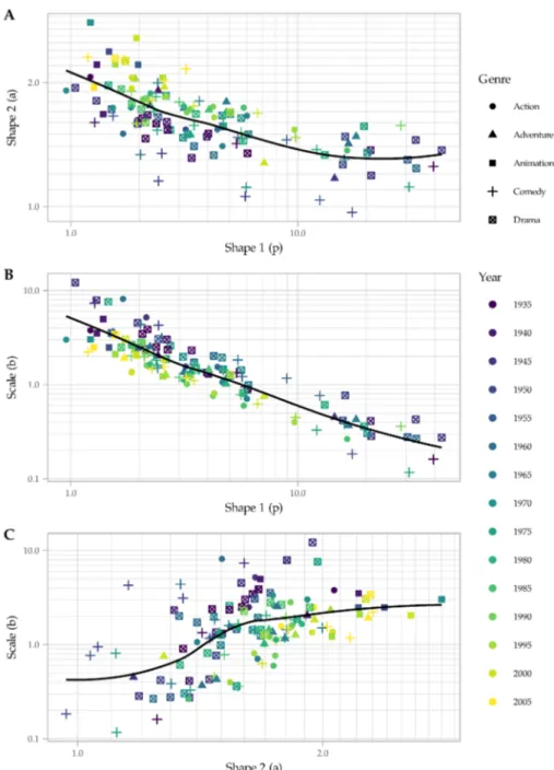
Figure 4 plots the parameters of the fitted Dagum distributions by year of release and genre. One of the key features to emerge is that most of the parameter values lie within a fairly narrow range indicating the homogeneity and consistency of Hollywood editing. Plotting the parameters on log-log scales shows there is a strong relationship between the two shape parametersp and a for most films but that this relationship does not hold for larger values of p (Figure 4.A); a strong power law relationship between the shape 1 ( p) and scale (b ) parameters (Figure 4.B); but a much weaker relationship between the shape 2 and scale parameters (Figure 4.C). The loess trendlines in Figure 4 indicate there is a sub-group of 22 films withp> 12, a ' 1.3, and b < 1, largely comprised of comedy and
drama films that tend to be more slowly edited and exhibit higher relative dispersion of their shot lengths than other films in the sample, with more variation around the median shot length than is evident elsewhere in the sample. Leaving this sub-group of films aside, we see that films released after 1975 tend to have highera and lower b parameters, respectively, than films released up to 1975, with the trendlines in Figure 4 splitting the main group of the sample. More recent films – i.e. those released since 1990 – tend to cluster together indicating a trend to similar shot length distributions over time. Again, this reflects the shift to a more rapid editing style in contemporary Hollywood cinema as the relative proportions of shots of shorter duration has increased and longer takes has decreased. There does not appear to be a clear trend in the value of the shape 1 parameter over time, with p related to the weight of the tails relative to the mass of the data. Changes in the two shape parameters of the Dagum distribution over time therefore characterise the polarization of shot lengths in Hollywood cinema, with the shift to an intensified continuity editing style resulting in the concentration of shot lengths in a narrower range of values and an increase in the relative extremity of the tails of the distributions.
There is a tendency for films that are better fitted by the lognormal distribution to be found on the left-hand side of Figures 4.A and 4.B, with low p values and high a and b values. An example of this tendency can be seen in the animated films in the sample, which show more similarity to one another than we see for films in other genres and which show no apparent difference between earlier cel-animated films and later digitally produced films. These films typically having among the lowest shape 1 parameters (p= 1.2−2.5) and among the highest values for the shape 2 (a = 1.6−2.8) and scale parameters (b = 1.2 − 4.9) and exhibit a consistency of style from Fantasia (1940) to Madagascar (2005) not evident in other genres. As Figure 5 shows, films such asThe Aristocats (1970) can still be well-modelled by the Dagum distribution but the lognormal distribution does appear to be a better choice for animated films.
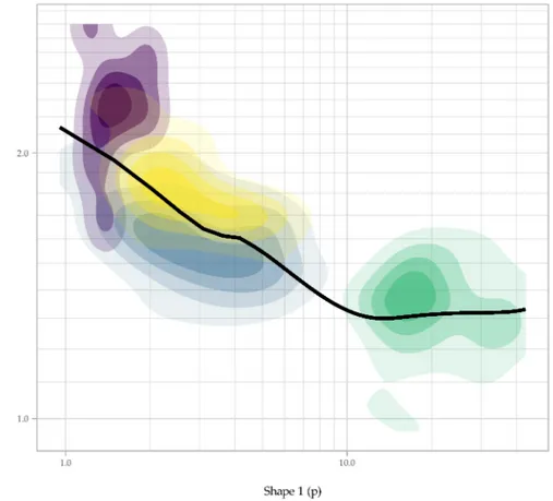
The shape of the distribution of shot lengths in a motion picture is the product of the relationship between thea and p parameters. Consequently, choice of parameters to produce a Dagum distribution as a model of shot lengths for automated video editing will depend on how filmmakers choose to construct that relationship. Figure 6 presents a 2-d density plot of four groups of films in the sample based on their shape parameters, indicating the concentration and range of values ofa and p for different editing styles. Using this map, filmmakers can select appropriate pairs of values according to taste, en-abling them to meet the competing demands of adherence to a set of stylistic norms and variability in editing between films by selecting parameters from the range of possible pairs for a given style. Although there is some overlap of the ranges for the classical and intensified continuity styles the concentrations are separated diagonally by the trend-line, signalling interaction between choices ofa and p for these editing styles. This is not the case for the other two groups of films. This plot makes the distinctiveness of the animated films in the sample evident, and the shape of the density region here indicates that choice ofa is crucial as values of p are relatively limited for this genre. Conversely, for films with high relative dispersion it is the choice of p that dominates the shape of
Figure 4 – Parameter relationships of the three-parameter Dagum distribution fitted to shot length data of 134 Hollywood films released from 1935 to 2005 (Source: Cuttinget al. (2010);http: //www.cinemetrics.lv/database.php), with loess trendlines.
Figure 5 – Probability density function (A), cumulative distribution function (B) and quantile-quantile (C) plots for fitted three-parameter Dagum and two-parameter lognormal distributions forThe Aristocats (1970).
Figure 6 – 2-d density plots of Dagum shape parameters for the four main types of films in sample a 134 Hollywood films released from 1935 to 2005. (Source: Cuttinget al. (2010);http://www. cinemetrics.lv/database.php).
the desired distribution as values ofa are limited. The value of the scale parameter can be determined based on the apparent power law relationship evident in Figure 4.B, where b' 4.58 × p−0.87.
5. CONCLUSION
In this paper I fitted the three-parameter Dagum distribution to shot lengths in Hol-lywood motion pictures. Based on the K-S statistics, the A-D statistics, the BIC, and visual inspection of the distributions, the Dagum distribution is a flexible model that well describes shot lengths in Hollywood motion pictures and generally provides a bet-ter fit than the two-paramebet-ter lognormal distribution due to its ability to model shot length distributions with a broad range of shapes. Animated films, however, appear to be better fitted by the lognormal distribution. These results can be used to inform the choice of model for automated video editing to produce sequences that more closely the editing practices of film editors based on the selection of the shape parameters appro-priate to a particular style of editing. I also identified a power law relationship between the skewness and kurtosis of shot lengths for films in the sample withν = 1.96, which is consistent with results reported in other fields though it is unclear why this relationship should hold for motion pictures as it does for natural systems.
REFERENCES
F. ÁLVAREZ, F. SÁNCHEZ, G. HERNÁNDEZ-PEÑALOZA, D. JIMÉNEZ, J. M. MENÉN
-DEZ, G. CISNEROS(2019). On the influence of low-level visual features in film
classifi-cation. PloS ONE, 14, no. 2, p. e0211406.
M. AUSLOOS, R. CERQUETI(2018).Intriguing yet simple skewness: Kurtosis relation in
economic and demographic data distributions, pointing to preferential attachment pro-cesses. Journal of Applied Statistics, 45, no. 12, pp. 2202–2218.
M. BAXTER(2014). Notes on Cinemetric Data Analysis. http://www.cinemetrics.
lv/dev/Cinemetrics_Book_Baxter.pdf. Online; accessed 26 August 2019. D. BORDWELL(2006). The Way Hollywood Tells It: Story and Style in Modern Movies.
University of California Press, Berkeley, CA.
J. E. CUTTING, A. CANDAN(2015). Shot durations, shot classes, and the increased pace
of popular movies. Projections, 9, no. 2, pp. 40–62.
J. E. CUTTING, J. D. LONG, C. E. NOTHELFER(2010). Attention and the evolution of
Hollywood film. Psychological Science, 21, no. 3, pp. 432–439.
C. DAGUM (2008). A new model of personal income distribution: Specification and
es-timation. In D. CHOTIKAPANICH(ed.),Modeling Income Distributions and Lorenz
M. L. DELIGNETTE-MULLER, C. DUTANG(2015).fitdistrplus: An R package for fitting distributions. Journal of Statistical Software, 64, no. 4, pp. 1–34.
C. DUTANG, V. GOULET, M. PIGEON(2008).actuar: An R package for actuarial science. Journal of Statistical Software, 25, no. 7, pp. 1–37.
Q. GALVANE, R. RONFARD, M. CHRISTIE(2015a). Comparing film-editing. In Euro-graphics Workshop on Intelligent Cinematography and Editing, WICED ’15, May 2015, Zurich, Switzerland. The Eurographics Association, pp. 5–12.
Q. GALVANE, R. RONFARD, C. LINO, M. CHRISTIE(2015b). Continuity editing for 3d animation. In Proceedings of the Twenty-Ninth AAAI Conference on Artificial Intel-ligence. pp. 753–761.
C. KLEIBER(1996).Dagum vs. Singh-Maddala income distributions. Economics Letters, 53, no. 3, pp. 265–268.
C. KLEIBER(2008). A guide to the Dagum distributions. In D. CHOTIKAPANICH(ed.), Modeling Income Distributions and Lorenz Curves, Springer, New York, pp. 97–117. C. KLEIBER, S. KOTZ(2003). Statistical Size Distributions in Economics and Actuarial
Sciences. John Wiley & Sons, Hoboken, NJ.
I. KOHARA, R. NIIMI(2013). The shot length styles of Miyazaki, Oshii, and Hosoda: A quantitative analysis. Animation, 8, no. 2, pp. 163–184.
M. LEAKE, A. DAVIS, A. TRUONG, M. AGRAWALA(2017). Computational video edit-ing for dialogue-driven scenes. ACM Transactions on Graphics, 36, no. 4, pp. 130–1. J. MCDONALD, J. SORENSEN, P. A. TURLEY(2013). Skewness and kurtosis properties
of income distribution models. Review of Income and Wealth, 59, no. 2, pp. 360–374. R CORE TEAM (2018). R: A Language and Environment for Statistical Computing. R Foundation for Statistical Computing, Vienna, Austria. URL http://www. R-project.org/.
A. E. RAFTERY(1995).Bayesian model selection in social research. Sociological Method-ology, 25, pp. 111–164.
R. RONFARD(2017). Five challenges for intelligent cinematography and editing. In Eu-rographics Workshop on Intelligent Cinematography and Editing, EuEu-rographics Associa-tion, April 2017, Lyon, France.
F. SATTIN, M. AGOSTINI, R. CAVAZZANA, G. SERIANNI, P. SCARIN, N. VIANELLO
(2009). About the parabolic relation existing between the skewness and the kurtosis in time series of experimental data. Physica Scripta, 79, no. 4, p. 045006.
J. R. SMITH, D. JOSHI, B. HUET, W. HSU, J. COTA(2017).Harnessing A. I. for augment-ing creativity: Application to movie trailer creation. In Proceedaugment-ings of the 2017 ACM on Multimedia Conference - MM ’17. ACM Press, Mountain View, California, USA, p. 1799–1808. URLhttp://dl.acm.org/citation.cfm?doid=3123266.3127906. C. TASKIRAN, E. DELP(2002).A study on the distribution of shot lengths for video
anal-ysis. In SPIE Conference on Storage and Retrieval for Media Databases. vol. 4315. N. VASCONCELOS, A. LIPPMAN(2000).Statistical models of video structure for content
analysis and characterization. IEEE Transactions on Image Processing, 9, no. 1, pp. 3–19.
P. H. WESTFALL(2014).Kurtosis as peakedness, 1905–2014. R.I.P. The American
Statis-tician, 68, no. 3, pp. 191–195.
SUMMARY
This paper demonstrates the three-parameter Dagum distribution provides a good fit for shot lengths in Hollywood films due to its ability to model a wide range of skewness and kurtosis values and a variety of tail behaviours by virtue of its two shape parameters. The fit of this distribution is better across films in the sample than the two-parameter lognormal distribution, though animated films are an important exception to this. These results can be applied to more closely replicate the editing practice of film editors when generating film sequences using automated editing software.