A geometric approach to the structure of complex networks

A geometric approach to the structure

of complex networks

Guillermo García Pérez

Aquesta tesi doctoral està subjecta a la llicència Reconeixement- NoComercial – CompartirIgual 4.0. Espanya de Creative Commons.

Esta tesis doctoral está sujeta a la licencia Reconocimiento - NoComercial – CompartirIgual 4.0. España de Creative Commons.

This doctoral thesis is licensed under the Creative Commons Attribution-NonCommercial-ShareAlike 4.0. Spain License.

P

H

D T

HESIS

A geometric approach to the

structure of complex networks

Author

G

UILLERMO

G

ARCÍA

P

ÉREZ

Advisors

P

. M

Á

S

D

. M

B

A geometric approach to the

structure of complex networks

M

U

B

P

ROGRAMA DE DOCTORAT EN FÍSICA

Autor

G

G

P

Directors

P

. M

Á

S

D

. M

B

Tutor

Acknowledgements

I have many reasons to be grateful to my advisors, M. Ángeles Serrano and Ma-rián Boguñá: for the trust you put in me with a fellowship, giving me the oppor-tunity to start a scientific career; for all the hours and selfless effort that you have dedicated to patiently guide and mentor me, always finding the time to discuss with me, and for everything that I have learnt from your expertise as a result; for the comfortable and active working environment—in which we have had more research ideas than we could possibly tackle—that has motivated me through-out these years; and for being always supportive when times were difficult, either personally or professionally. Thank you, I am very lucky to have studied my PhD with you, and I hope that we continue to work together.

I am also very thankful to Antoine Allard, with whom I have collaborated much these years. Antoine, it has been great working with you, and thanks for everything you have taught me. I also want to thank Francesco, Michele, Muhua, Nikos and Roya for the good time working together.

I would like to thank Profs. Sabrina Maniscalco and Jyrki Piilo for allowing me to stay at the Turku Quantum Technology group as a visiting PhD student. I am also grateful to them, as well as to Johannes Nokkala, for our collaboration: I really enjoyed it. I had a great time in Finland, and for that I must thank everyone at the UTU Theoretical Physics Department.

Thanks also to my colleagues at UB for the good times and the interesting discussions. I specially thank Elisenda, Jan, Michele, Oleguer, Pol and Xavi for their valuable advice and comments. I also acknowledge Albert Díaz for manag-ing the ClabB as well as many group activities.

It has been quite stimulating to witness how Quadrívium, which started as a few of us giving some outreach talks every now and then, has grown during these years. I must acknowledge Blai G., Blai P., Gian, Matt and Nahuel for it.

I am deeply thankful to Marta, probably the person who knows me best, for always helping me to pursue my goals, even in the hardest moments. I also want to thank my friends, especially Elisa, for the scientific conversations and for their help whenever I needed it during this period.

Finally, I want to express my gratitude to my family, especially to my parents Margarita Pérez and Mario García, who encouraged me to return to my studies many years ago and unconditionally supported me along the path. I owe you many things, but I take this occasion to thank you for helping me to find out what I really wanted to do and to make it possible.

Contents

1 Introduction 1

1.1 Complex networks . . . 1

1.1.1 The universal properties of real networks . . . 3

1.1.2 Network models. . . 7

1.2 Hidden metric spaces . . . 9

1.2.1 Similarity, geometry, and clustering . . . 10

1.2.2 Geometric network models . . . 10

1.2.3 Embedding of real networks and navigability . . . 14

1.3 Outline of the thesis . . . 17

2 Static geometric models and embeddings of networks 21 2.1 Similarity space as a sphere . . . 21

2.2 TheS1model . . . 22

2.3 TheH2model . . . 25

2.3.1 Isomorphism between theS1and theH2models . . . 25

2.3.2 Specifications . . . 26

2.4 Embedding methods . . . 27

2.4.1 Algorithm for large networks . . . 28

2.4.2 Algorithm for sequences of small networks . . . 31

2.5 Beyond angular homogeneity . . . 34

2.5.1 Geometric Preferential Attachment in theS1model . . . 36

2.6 Higher-dimensional similarity space . . . 40

2.6.1 TheSD model . . . 40

2.6.2 Clustering and dimensionality . . . 43

2.7 Discussion . . . 46

2.8 Additional information. . . 47

2.8.1 The distribution of distances on a D-sphere . . . 47

3 The World Trade Atlas 1870–2013 49 3.1 Beyond detached bilateral flows and geographic distance . . . 49

3.2 The World Trade Web as an undirected complex network . . . 51

3.2.1 Data and network reconstruction . . . 54

3.3 Mapping the World Trade Web . . . 60

3.3.1 A gravity model for trade channels . . . 60

3.3.2 Hyperbolic maps of WTW backbones . . . 62

3.4 Trade since the 19th century . . . 66

3.4.2 Detecting communities in WTMs: the CGM method . . . 69

3.4.3 WTM communities versus PTAs . . . 71

3.5 Discussion . . . 76

4 Geometric renormalization of complex networks 79 4.1 The problem of scales in complex networks . . . 79

4.2 The Geometric Renormalization Group transformation . . . 80

4.3 Evidence of geometric scaling in real networks. . . 82

4.4 Expected scaling in geometric models . . . 86

4.4.1 Transforming the parameters of the model . . . 86

4.4.2 Flow of the average degree . . . 90

4.4.3 Connectivity phase diagram . . . 93

4.5 Applications . . . 94

4.5.1 Smaller-scale replicas for efficient dynamics simulation . . . 94

4.5.2 A multiscale navigation protocol in hyperbolic space . . . 98

4.6 The partition function in hyperbolic space . . . 101

4.7 Discussion . . . 103

4.8 Additional information. . . 104

4.8.1 Exact behaviour of the average degree for r = 2 . . . 104

4.8.2 Renormalization in higher dimensions . . . 107

5 The geometric nature of weights in real complex networks 111 5.1 Beyond binary networks . . . 111

5.2 Interplay between weights and triangles in real networks . . . 112

5.3 A geometric model of weighted networks . . . 115

5.3.1 General properties of the model . . . 117

5.3.2 The one-dimensional version. . . 121

5.3.3 The effect of the underlying geometry . . . 122

5.4 Hidden metric spaces underlying real weighted networks . . . 124

5.4.1 Inference via the triangle inequality . . . 126

5.4.2 Reproducing real networks . . . 128

5.5 Discussion . . . 134 5.6 Calculation details . . . 136 6 Conclusions 139 A List of publications 145 B Resum en català 147 References 153

C

HAPTER

1

Introduction

1.1 Complex networks

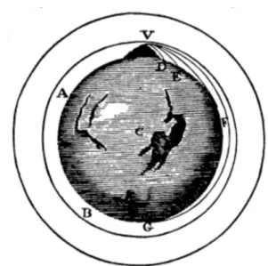
The last three centuries have witnessed an explosive development of scientific knowledge. In 1687, Sir Isaac Newton published the Principia [120], a book in which he introduced the fundamental laws that govern the motion of bodies. His important discoveries allowed, for the first time in human history, to explain and predict in precise mathematical terms the motion of any body using three simple principles. Even more strikingly, not only did Newton explain how bod-ies move when forces act upon them, but also how bodbod-ies exert gravitational forces one onto another. He even devised a beautifully simple thought experi-ment some years later [121], depicted in Fig.1.1, which illustrates how his dis-coveries unify the motion of celestial bodies, ever before regarded as divine en-tities, and the motion of regular, mundane earthly bodies. Newton imagined a cannon, the power of which can be regulated, located at the summit of a moun-tain; as the velocity with which the cannonballs are shot parallel to the ground increases, the trajectories described by them become further-reaching until, for some critical initial speed, they orbit the planet, just like the Moon orbits the Earth. In other words, the orbit of the Moon around our planet was no longer to be considered different in nature from that of an everyday object falling to the ground.

Not surprisingly, the great success of being able to reduce so many seemingly diverse phenomena to a few principles paved the way to reductionism, which has ever since been doubtlessly fruitful in physics. This approach is guided by the idea that it is sufficient to understand the elementary processes taking part in a system in order to explain its observed behaviour. Nevertheless, and despite the long list of achievements of reductionism—and the ones still to come—, it might not always lead to a complete understanding of Nature. While it is cer-tainly true that many systems can be analyzed in terms of the basic rules gov-erning each of their parts—like, for instance, the macroscopic behaviour of an ideal gas can be derived from the assumption that its constituent atoms obey Newton’s laws of motion—, that might be possible for some particular systems only. For example, it is hard to imagine how one could explain human behaviour from first physical principles, even though all processes taking place in a human body are driven by them.

Figure 1.1: Netwon’s cannonball. Thought experiment devised by Newton to illustrate how an attractive force between massive objects explains both the falling of objects and planetary orbits. The cannonballs are shot parallel to the ground from the summit of the mountain. In the absence of air, they become satellites provided sufficient initial velocity.

In the systems that we call complex, which exhibit behaviours that are not ex-pected from the driving principles applicable to their elements, the interaction patterns between its constituent units are—at least partly—responsible for these emergent phenomena and, therefore, they need to be accounted for as well. In other words, besides knowing the laws governing each part of the system, it is also imperative to know how these different parts interact, which forces us to drop the reductionist approach and turn towards a holistic description. This is where complex networks become essential.

Complex networks [118,50, 57] represent the interaction patterns of com-plex systems in terms of graphs, mathematical objects conceived by the great

mathematician Leonhard Euler [62]. They are composed of nodes, or vertices,

representing distinct parts of a system, and edges, or links, representing their pairwise interactions. Clearly, such an abstract description can be applied to a vast variety of systems, and they are indeed used in many different fields of knowledge, like sociology, biology, technology, mathematics or physics, to name a few. For instance, social networks usually represent interactions of some sort— like friendship or collaboration—between people, whereas biological networks range from descriptions of metabolisms to interactions between neurons. In any case, the generality of the concept of network and the importance of considering interactions in many fields make complex networks an appealing approach to

1.1. Complex networks 3

many sciences which, in turn, makes network science one of the most transver-sal lines of research nowadays.

During the last 20 years, since the first papers on network theory were pub-lished, many real networks have been measured, which has allowed researchers to characterize their topologies. Remarkably, although they are far from be-ing regular lattice-like structures or purely random and unstructured graphs, it has become clear that there are some ubiquitous features exhibited by networks from completely different domains [40,166].

1.1.1 The universal properties of real networks

Complex networks are usually classified according to the nature of their links. Networks are called simple if their links are binary, that is, if they do not have any attributes other than their existence, whereas they can be weighted if there is an intensity assigned to every link, or directed if the links have a directional-ity. Mathematically, a network is usually represented in terms of its adjacency matrix A, whose elements ai j ≡ (A)i j contain the information regarding the

connections between every pair of nodes i and j . Hence, for simple networks,

ai j= aj i= 1 if both nodes are connected and ai j= aj i = 0 otherwise. In directed

networks, however, the adjacency matrix is not symmetric, while in weighted networks, the adjacency matrix elements are positive real numbers. In the latter case, it is frequent to use the notationωi j instead of ai j.

In this thesis, we mainly focus on simple and weighted networks, so we re-strict our account of network properties in this section to these two classes of graphs. We first review the main topological features, which are only related to the existence of links and, secondly, the weighted properties, which are defined for weighted networks only.

1.1.1.1 Topological properties

The first feature of real networks to be identified was degree heterogeneity [56,

11,63,87]. The degree of a node i , typically referred to as ki, is the number of

links reaching it, that is, its number of neighbours. In real networks, this quan-tity is very heterogeneously distributed, since most nodes have very low degree, while a very small amount of nodes are connected to a macroscopic fraction of the system. More precisely, the degree distribution, defined as the probability for a randomly chosen node in the network to have k neighbours, scales as a power-law

P (k) ∼ k−γ, (1.1)

where the exponentγ, which measures degree heterogeneity, is usually found

Eq. (1.1) diverge as the size of the network N → ∞, which implies that, even if the average degree is well defined (finite), it does not represent a measure of typical degrees in the network, since fluctuations are very large (infinite in the thermodynamic limit). This is the reason why real-world networks are called

scale-free networks. Real networks are also sparse, meaning that their average

degrees are small as compared to the system size1.

100 ₁₀1 ₁₀2 k 10−3 10−2 10−1 100 Pc (k ) a 100 ₁₀1 ₁₀2 k 10−1 100 ¯c( k ) b 100 ₁₀1 ₁₀2 k 10−1 100 hk i hk 2i knn (k ) c 1 2 3 4 5 l 0.0 0.2 0.4 0.6 0.8 1.0 P (l ) d

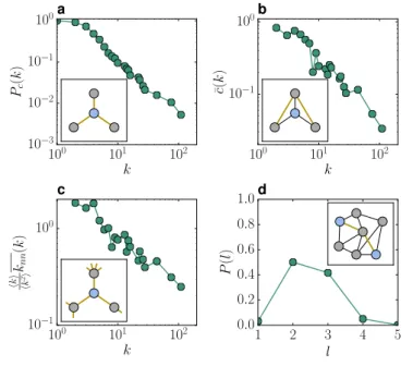
Figure 1.2: Topological properties of a real network. The green curves

repre-sent different features of the World Trade Web network in 2013 (see Chapter3

for details). The insets illustrate the different quantities under scrutiny. a, Com-plementary cumulative degree distribution Pc(k) =P∞_k0_=kP¡k0¢ representing the

probability for a randomly chosen node in the network to have a degree larger than or equal to k, which is less noisy than P (k). b, Clustering spectrum, that is, average clustering computed over nodes of the same degree. As an example, the blue node in the sketch has c = 2/3. c, Normalized average nearest neighbours degree averaged over all nodes in every degree class. The normalization factor ­k2_{® /〈k〉 leaves this curve fluctuating around one for uncorrelated networks. In} this case, however, the network shows a clear disassortativity. The blue node in the inset has average nearest neighbours degree 10/3. d, Distribution of short-est path lengths. Despite the size of the network, N = 189 nodes, the most likely distance is l = 2, whereas very few pairs are separated by more than 4 hops. In the sketch, the two blue nodes lay at distance l = 2.

1_{The definition of sparseness is more precise in the context of network models, in which} net-work size N can be controlled. We say that a model generates sparse graphs if their average degree is independent of N .

1.1. Complex networks 5

Beyond the degrees of single nodes, some structures involving more nodes are also commonly found in real networks. In particular, the presence of trian-gles, or transitive connections, is much higher in real networks than predicted by most network models [111], as we will see in the next section. Triangles can be quantified in networks through the so-called clustering coefficient. Given a node

i with degree ki> 1, its clustering coefficient is defined as the probability for two

randomly chosen neighbours of i to be connected. This quantity is computed as

ci =

2ni

ki(ki− 1)

, (1.2)

where ni is the number of connections among neighbours of i and the

fac-tor 1₂ki(ki− 1) accounts for the maximum possible number of links among the

neighbours of i . Clustering is often represented by its spectrum, that is, the av-erage clustering of nodes of a given degree (see Fig.1.2b).

Global regularities are also observed in real topologies. Given a pair of nodes

i and j in a graph, the length of the shortest path, that is, the shortest sequence

of nodes with i and j as endpoints such that every pair of consecutive elements are connected (if there is any), defines a distance between the nodes. Indeed, this distance fulfils all the properties of a metric space: it is positively defined, equal to zero if and only if j = i , symmetric and it satisfies the triangle inequality,

di j≤ di l+ dl j, ∀l . (1.3)

This last property can be explained as follows. Since by definition no path can be shorter than the shortest path, the path resulting from the concatenation of the shortest paths from i to l and from l to j , the length of which is given by the right-hand side of the above inequality, cannot be shorter than di j. In real

networks, the average distances computed over all pairs of nodes are extremely short and scale as ¯d ∼ log N with the system size. This is called the small-world

property, and it was experimentally discovered on social networks in the 1960’s by Milgram [163]. Later on, it was also found that scale-free networks are

ultra-small [49], with a scaling given by ¯d ∼ loglog N . In both cases, the diameter of the

network D, defined as the longest shortest path, scales as D ∼ log N , which im-plies that the fluctuations of topological distances are small as well. In Fig.1.2d,

we show their distribution in the World Trade Web.

Some networks also present degree-degree correlations. For instance, tech-nological systems are usually disassortative [107], which means that low-degree nodes tend to connect to high-degree nodes and vice-versa. Social systems, on the other hand, usually exhibit the opposite assortative behaviour [53], accord-ing to which there is a positive correlation between the degree of a node and that of its neighbours. These correlations are typically measured in terms of the aver-age degree of the neighbours of nodes of a given degree, as in Fig.1.2c. Although

degree-degree correlations are not universal, in the sense that networks can be assortative, disassortative or even uncorrelated, it is an important structural fea-ture used to characterize real topologies.

Most real networks also present a clear community structure, which means that nodes can be partitioned into groups—communities—such that the density of connections among nodes within the same community is higher than among nodes belonging to different communities [117,137, 14]. Identifying the opti-mal partition into communities for a given network, i. e. the one that maximizes the link density within communities, has been a very active topic of research in network science.

It is worth pointing out that these are not the only structural features which have been recognized in real-world networks. For instance, they have also been studied in terms of motifs [111], quantifying the density of small subgraphs in them, of k-core decompositions [10], assessing the structure of the subgraphs in which all nodes have degree larger or equal to k, and even in terms of between-ness, measuring the number of shortest paths passing through a node or a link. Interestingly, all these properties seem to be reproduced by random networks as long as they have the same degree distribution, degree-degree correlations and clustering coefficient [126].

1.1.1.2 Weighted structure

In weighted networks, the local weighted structure of nodes is encoded in their

strength, defined as the sum of the weights of all links reaching it. In some sense,

it is the weighted equivalent to the topological degree and, as their topological counterparts, strengths are also power-law distributed in real networks,

P (s) ∼ s−ξ. (1.4)

Furthermore, another feature broadly observed in real datasets is a non-linear relation between strengths and degrees [20,136,22],

¯

s(k) ∼ kη, (1.5)

where ¯s(k) is the average strength of nodes with degree k andη is usually larger

than 1. Notice that this observation is not compatible with the trivial coupling between weights and topology, which leads to

¯

s(k) = 〈ω〉k, (1.6)

1.1. Complex networks 7

1.1.2 Network models

The fact that many real-world networks from utterly different origins share such important similarities suggests that there might be some general mechanisms driving their formation and evolution. In network science, a great deal of ef-fort has been devoted to unveiling and identifying what those principles are by proposing network models.

A network model is a set of rules defining the generation process of a graph; the goal is, therefore, to find a model with a minimal set of ingredients capa-ble of reproducing all the aforementioned network properties: scale-free degree distribution, sparseness, high clustering, small-world property and community structure. Indeed, such model would allow us to answer the question of why those features are ubiquitous.

It is important to note that there is a random component in most real net-works. This is a rather expected statement if we think in social terms, which are probably more intuitive to us; even if the decision to establish a relationship of some sort with someone is not purely random, there is randomness, at least, in who we have the chance to establish a connection with. Consequently, if we aim at modelling complex networks, it seems reasonable to adopt the approach of designing random models.

In a random model, the set of rules dictates the probability with which the events that generate the network happen, rather than specifying which particu-lar events happen. Therefore, a given random model with a given initial condi-tion or model parameters does not generate a single network, but a whole en-semble of networks, each of them with some probability, as opposed to a deter-ministic model in which the resulting network would be uniquely determined.

In addition to the considerations regarding the randomness of the approach, it is also important to distinguish between growing and static models. A growing model aims at explaining how complex networks grow in time, that is, how their topological structures emerge during the network-formation process. Typically, in growing models, nodes are added sequentially and the model specifies with what probability they connect with already existing nodes. Static models, on the other hand, focus on defining realistic ensembles of networks with a fixed set of nodes. In the rest of this section, we will briefly review several random models of particular importance in the development of network theory.

The first random model of networks was the Erd˝os-Rényi model [61, 60],

which generates completely random graphs. In this static model, for a given size N , E edges are randomly and uniformly distributed among the N (N − 1)/2 pairs of nodes. There is also a less constrained version of this model in which the number of links E is not fixed, but every pair of nodes has a probability p of being connected (the same for all pairs), which fixes the average number of

edges 〈E〉 [76]. In any of the two versions, the resulting graphs are small-world, but their degrees are homogeneously distributed and the clustering coefficient vanishes as N → ∞ if the average degree 〈k〉 is fixed. These two properties are easy to understand in the second and less restricted version. Since all links are identically and independently distributed, degrees follow a Binomial distribu-tion with mean p (N − 1). As for the clustering, notice that the probability for a pair of neighbours of some node to be connected is simply p, which scales as

p ∼ (N − 1)−1 for fixed p (N − 1). Hence, this model shows that real-world

net-works are not purely random, but some underlying mechanisms must be re-sponsible for degree heterogeneity and clustering.

The explanation of degree heterogeneity came by the hand of what is now commonly known as the preferential attachment mechanism, encoded in the

Barabási-Albert model [17]. In this growing network model, nodes are added

sequentially to the network and they establish a fixed number of connections

m with the already existing nodes. However, instead of choosing them with

equal probability, they tend to connect to higher-degree nodes with higher like-lihood. This simple rule, which implies that popularity plays a central role in the network-formation process, indeed results in power-law degree distributions. Nevertheless, this model presents a null clustering coefficient in the thermody-namic limit, so preferential attachment cannot be the only mechanism taking part in the evolution of real networks.

Although the Barabási-Albert model explains scale-freeness, it is not the only model capable of generating power-law degree distributions. There is yet an-other very important model in network science that allows to generate networks with a predefined target degree sequence but which are random in all other re-spects: the Configuration Model [37,24]. In this static model, every node i is assigned ki stubs, or half-links, and the network is constructed by randomly

se-lecting pairs of stubs to form the links (avoiding pairs of stubs belonging to the same node or to two already connected nodes to be chosen in order not to gen-erate networks with self-loops or multiple connections). Clearly, in the resulting network, every node has degree ki by construction. As in the case of the

Erd˝os-Rényi model, there is also a less constrained version, also known as the Soft

Con-figuration Model, in which every node is assigned an expected degree ki and

every pair of nodes is connected with a probability proportional to the product of them, pi j ∝ kikj. As in the case of the last two models, the Configuration

Model also has a vanishing clustering coefficient for large networks.

Finally, the small-world property was also explained in the early days of net-work theory by means of the Watts-Strogatz model [166]. In this model, N nodes are placed on a ring and connected to their k nearest neighbours, hence forming a regular ring-like lattice. Then, every link is visited and, with probability p, it is rewired, that is, one of its endpoints is moved to another randomly chosen node

1.2. Hidden metric spaces 9

in the network. With this simple rewiring mechanism, which generates short-cuts across the system, the model undergoes a transition from the non-small-world to the small-non-small-world regime as p is increased. Thus, this model identified randomness as an important element determining the structural properties of real networks. Contrarily to the models introduced so far, the Watts-Strogatz model does exhibit strong clustering that remains from the original lattice-like graph. However, degrees are homogeneous.

As for weighted networks, many models have been proposed to explain their observed properties. For instance, growing network models [27, 21, 174, 99,

13, 176, 165, 103] focus on identifying the basic rules driving the growth of weighted networks, usually in the form of a weighted preferential attachment. The maximum-entropy class of models [108, 70, 71, 144, 145], on the other hand, aims at describing real weighted structures in terms of maximally random graphs with a minimal set of constraints. Nevertheless, none of these models is able to reproduce simultaneously the topology and weighted structure of real weighted complex networks.

1.2 Hidden metric spaces

As we have seen in the previous section, although the canonical models in net-work science reveal some of the main mechanisms shaping the topology and weighted structure of real networks, they are not capable of incorporating all the ingredients in a simple set of rules. Furthermore, none of them provides a simple ontological explanation for the origin of clustering, in the same terms as prefer-ential attachment provides a reasonable explanation for degree heterogeneity.

Ten years ago, the idea of similarity between nodes as a plausible source of clustering was introduced by Serrano, Krioukov and Boguñá [152]. Remarkably, their considerations opened the path to a geometric understanding of complex networks that, besides yielding models capable of reproducing the observed fea-tures of real-world networks [152,94], provides us with new tools and techniques for their analysis and efficient navigation. This section presents a brief intro-duction to the hidden metric spaces approach to complex networks. After dis-cussing the basic concepts, we introduce the different static and growing geo-metric models and discuss how these allow to construct maps of real networks that can be used to analyze them from a novel perspective as well as to navigate them efficiently.

1.2.1 Similarity, geometry, and clustering

As we saw when we introduced the preferential attachment mechanism, scale-freeness emerges from the predilection of new nodes entering the system to con-nect to already existing ones based on their degrees, i. e. on their popularities. Nevertheless, it seems reasonable to assume that popularity might not be the only driving force in the connection-formation process. We could indeed pre-sume that the different parts conforming the system, the nodes, are not all equal to one another, but that they are equipped with some intrinsic properties other than popularity, and that the similarity between these intrinsic properties also plays a role in the probability for two nodes to interact. This simple yet reason-able assumption is suitreason-able to be described in geometric terms, as we shall see.

To understand why geometry might indeed be adequate for the description of the similarity between nodes, we should first recognize a very important prop-erty of similarity: transitivity. If two nodes A and C are both similar to a third node B , then A and C should also be similar to one another. Now, suppose that the space of the nodes’ intrinsic properties is a metric space, such that the dis-tance between two points in the space is a measure of their dissimilarity, that is, the closer two points lay in the space, the more similar the intrinsic properties represented by those points are. Then, the transitivity of similarity is automati-cally incorporated in the structure of the metric space as a result of the triangle inequality

dAC≤ dAB+ dBC, (1.7)

which, in terms of similarity, admits the following reading: the dissimilarity be-tween nodes A and C is bounded by the sum of the dissimilarities of both nodes to node B .

In our network-modelling context, the transitivity of similarity—or, equiva-lently, of similarity-distance closeness—represents a natural source of cluster-ing. If similarity takes part in the probability for two nodes to connect, then two nodes A and C near in similarity space to node B should be connected to B with high probability. Since, in light of Eq. (1.7), A and C must also be near in similar-ity space, they should have a high probabilsimilar-ity of being connected as well, thus yielding a non-zero clustering coefficient for node B . Figure1.3illustrates how triangles emerge among nearby nodes in the underlying space.

1.2.2 Geometric network models

In order to explore the geometric origin of clustering in real networks in precise mathematical terms, we need network models based on underlying similarity spaces. In this section, we introduce the main geometric network models pro-posed during the last years.

1.2. Hidden metric spaces 11

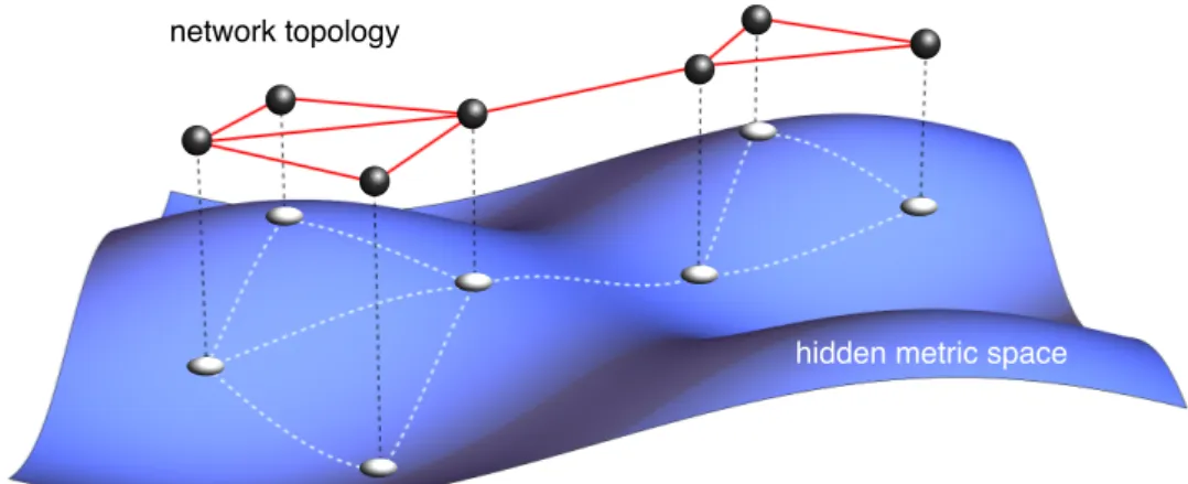
hidden metric space

network topology

Figure 1.3: Illustration of the connection between network topology and

hid-den metric spaces. The blue surface represents an arbitrary metric space on

which several nodes are scattered. The distance among them is given by the length of the geodesics, or shortest curves, drawn as light dashed lines on the surface. Connections are established among nearby pairs only, giving rise to re-sulting topology depicted in the upper layer. Notice that topological triangles appear naturally as a consequence of the closeness in the hidden metric space.

The first model based on an underlying geometry to be proposed was theS1

model2[152]. In this model, every node is assigned two hidden variables, a

hid-den degree and a coordinate on a circle abstracting the simplest geometry for a similarity space. The connection probability between two nodes then depends on the ratio between their distance along the circle—their similarity—and the product of their hidden degrees—their popularities. Therefore, this model re-sembles a gravity law for connectivity, in the sense that the likelihood for two nodes to be connected increases with the product of their “masses”, the hidden degrees, and decreases with the distance among them. This simple model gen-erates very realistic topologies regardless of the specific form of the connection probability function, as long as it is a sufficiently fast decaying function of the aforementioned ratio. Moreover, every node’s degree becomes proportional to its hidden degree, which confers the model a high level of control over the de-gree distribution. As we will see when we discuss the mathematical details of the model, two additional global parameters enable to control the average de-gree and clustering of the resulting networks as well. It is worth mentioning that

2_{In fact, it was proposed as a model in arbitrary dimensions, although it has ever since} partic-ularized to its one-dimensional version for simplicity. We explore the general version in detail in Section2.6.

the model has also been extended to bipartite networks in which one mode ex-hibits a heterogeneous degree distribution while, in the other mode, degrees are

homogeneous [155].

Interestingly, it was later discovered that hyperbolic geometry emerges from theS1model [93,94]. By mapping every node’s hidden degree into a radial coor-dinate appropriately, with high-degree nodes closer to the origin of the coordi-nate system than low-degree nodes, they all lay on a two-dimensional finite disk, and the connection probability becomes a function of the distance separating them only; this distance, however, is not the familiar Euclidean distance but, in-stead, that of the negatively curved homogeneous hyperbolic space. Therefore, theS1model is isomorphic to a purely geometric model, theH2model, in which

nodes are sprinkled on a hyperbolic disk and then connected with a probability that decreases with the distance among every pair of them. It is important to note that, in this purely geometric representation, geometry does not only en-code similarity distances, but it includes the popularity dimension (degrees) as well in a sole distance metric.

Both theS1and theH2models will be explained in detail in Chapter2. How-ever, it might be beneficial to give some intuition about hyperbolic geometry and its interplay with complex topologies at this point. Hyperbolic space is a metric space with constant negative curvature [45]. Unfortunately, contrarily to its pos-itively curved counterpart—the two-dimensional sphere—the two-dimensional hyperbolic plane cannot be completely embedded isometrically as a surface in three-dimensional Euclidean space, which hinders its visualization and makes it less intuitive. Nevertheless, we can still grasp some intuition about this geom-etry by writing down the metric tensor explicitly in the coordinate system of the so-called native representation, or polar coordinate system, of hyperbolic space, which will be the only one used in this thesis. In these coordinates, every point in the space is given a radial coordinate standing for the distance to the (arbi-trary) origin of the space, as well as an angular coordinate between zero and 2π. The metric then reads

ds2= dr2+ sinh2r dθ2. (1.8)

By comparing it to the metric of the familiar Euclidean two-dimensional plane in polar coordinates, ds2= dr2+r2dθ2, we can immediately notice that the perime-ters of hyperbolic circles grow much faster with their radii than Euclidean circles. In particular, they grow exponentially, with a scaling given by the hyperbolic sine in Eq. (1.8). Naturally, the areas of disks also scale exponentially with their radii. Now, in theH2model, nodes are sprinkled with a fixed (and quasi-uniform) density, as will be explained in detail in the next chapter. This means that the number of nodes at distance smaller than r from a given node is proportional to the area of the hyperbolic disk of radius r centred at the node and, hence,

1.2. Hidden metric spaces 13

scales exponentially with r ; this is fully consistent with the small-world prop-erty, as a result of which the number of nodes at a given topological distance d from any node scales exponentially with d . Besides explaining small-worldness, clustering is immediately encoded in the triangle inequality, so all the discussion presented in Section1.2.1can be applied here as well. Finally, we can give an in-tuitive interpretation of degree heterogeneity in this context. As we will see in the next chapter, nodes tend to establish connections with other nodes at distance smaller than the radius of the hyperbolic disk ˆR (see Eq. (2.12) for details). Con-sequently, a node with very small radial coordinate is close to the point laying at distance smaller than ˆR from all the nodes in the system: the origin. Therefore,

nodes near the origin tend to have very high degrees. Nodes in the periphery, on the other hand, can only connect to other nodes that are either near the origin or peripheral but very close angularly. This last point can be seen from the met-ric: in the periphery of the disk, a very small angular separation becomes a very large hyperbolic distance. Therefore, nodes at large radial coordinates can only connect to a much more restricted set of nodes.

This thesis strongly relies on these two static geometric models, and the iso-morphism between them is repeatedly used throughout. Nevertheless, there are also two growing geometric models which we present here for completeness.

The Popularity versus Similarity Optimization model (PSO) [133] is based on the following assumptions. First, the popularity of a node at a given growth-time is determined by its age, that is, how long ago it appeared into the system; hence, older nodes should receive more connections from newcomer nodes. In other words, there is a preferential attachment process. Second, newly added nodes do not choose their neighbours according to their popularity only, but they also take similarity, abstracted as an angular coordinate, into consideration, hence-forth generating clustering in the resulting networks. In the PSO model, when a node enters the system, it connects with a fixed number m of nodes that are maximally popular or similar to itself, where m regulates the average degree. Re-markably, by mapping each age to a radial coordinate appropriately, the model can be interpreted as nodes connecting to the m closest nodes in hyperbolic space. Furthermore, allowing the popularity of nodes to fade away over time confers the model control over degree heterogeneity, whereas the level of clus-tering can be regulated by adding some randomness to the selection of neigh-bours.

As we discuss in the next section, when we unveil the hidden similarity space coordinates of nodes in real networks through a process that we call embedding, we observe a non-uniform angular distribution of nodes, a phenomenon inti-mately entangled with the community structure of the network. To account for these geometric communities, a model based on the PSO was proposed: the

not appear with uniform angular density on similarity space; instead, the prob-ability for a new node to appear at a given coordinate increases with the amount of nodes in the vicinity of such point. Hence, there is a geometric preferential at-tachment in similarity space that provides a plausible explanation for the com-munity structure of real networks: the intrinsic properties of nodes, defining their position in similarity space, are influenced by the properties of already ex-isting nodes, as they tend to mimic features which are frequent in the system.

Notice that theS1model shares some similarities with the gravity-law ap-proach to trade in economics [162, 26, 158] to predict trade volumes, whereas the H2 model resembles latent space models [109, 110], conceived to explain homophily and similarity in social systems.

1.2.3 Embedding of real networks and navigability

One of the most interesting possibilities that geometric models offer is the em-bedding of real-world networks into hidden metric spaces. To that end, we con-sider the following problem: given a network, and assuming its geometric origin, can we find its embedding on a hidden metric space, that is, can we infer the hid-den variables and model parameters that best describe the observed topology? This question has been proved to have a positive answer in general, although it poses some technical challenges. In this section, we briefly discuss the most commonly adopted methods to tackle this problem and elaborate on the possi-bilities that the resulting maps of real systems open.

A very widely used method to address the problem of geometric-information inference is likelihood maximization [35,155,2,30]. The basic idea is to find the set of hidden variables and model parameters that maximize the likelihood for the observed network to be generated by the model. This is indeed the general scheme followed to obtain all the embeddings in this thesis, so the procedures will be detailed in Chapter2. However, it is worth mentioning that this embed-ding scheme is not representative of all currently available methods. Several new approaches to tackle this problem apply machine learning algorithms to find the angular coordinates, disregarding the likelihood completely [8,115]. Some other methods follow a pure likelihood-maximization strategy making use of the growing models instead of the static versions [134].

What makes it worth overcoming the technical difficulties of network em-bedding is applying the technique to real-world networks. If we adhere to the hypothesis that similarity between nodes influences the observed topolo-gies of real networks, we can interpret the coordinates of nodes obtained from the embedding as their positions in the underlying similarity space. In other words, embedding a network onto a metric space provides us with a map of the system’s similarity space, which would otherwise remain hidden. A

scep-1.2. Hidden metric spaces 15

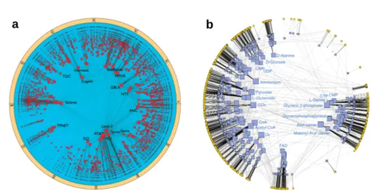
Figure 1.4: Hyperbolic representations of two real-network embeddings.

Nodes are represented by squares and links by lines between them. Every node is assigned a radial coordinate representing its popularity, or degree, such that high-degree nodes are near the centre (see Section2.3for further details). An-gular coordinates account for the positions of nodes in similarity space, so the boundary of the disk is theS1model metric space. Notice that both angular dis-tributions are far from being homogeneous, as they exhibit large gaps and highly populated angular regions. a, The Internet Autonomous Systems network. Ev-ery node is an Autonomous System, a subnetwork in the physical network of the Internet, taking part in the information-routing process. The embedding reveals a clear correlation between nodes and their geographical location [35].

b, Metabolic network of the Escherichia coli. Every node is a metabolite and

the connections among them represent their participation into common reac-tions. In this case, angular inhomogeneities are closely related to metabolic pathways [155].

tical reader, however, might argue that maximizing the likelihood for any net-work, including graphs without a geometric origin, would yield a set of hidden coordinates, which in turn implies that the coordinates obtained from the em-bedding of real networks could be meaningless, in the sense that they need not have a similarity-coordinate interpretation. However, during the last ten years, much evidence supporting precisely the opposite claim has been accu-mulated [35,155,82,2,3,4], including many of the results in this thesis.

A notable characteristic of the angular coordinates obtained from the em-bedding or real networks is non-uniformity; we usually find angular regions where the density of nodes is higher than average followed by large empty gaps separating these regions (see Fig.1.4). The reason for the appearance of these denser areas is that, within any of them, the link density is higher than aver-age, so they are caused by the community structure of the network. In order

for the model to encode this higher link density, the average angular distance between nodes within each community needs to be shorter, thus forming these angular correlations in the embedding. Moreover, the resulting angular distribu-tion usually has a very evident interpretadistribu-tion in terms of similarity. For instance, in the embedding of the Internet [35], the angular communities were found to be highly correlated with geographic localization, while in the geometric analy-sis of the Human and E. Coli metabolisms [155], the pathways could be clearly identified in different angular sectors. Notice, nevertheless, that the embedding process is completely blind to this information, as it simply maximizes the like-lihood function based on the adjacency-matrix elements.

In addition to revealing the hidden similarity and, consequently, the com-munity structure of networks at a glance, the embedding of real networks is a valuable resource for efficient network navigation as well [36,33]. This is espe-cially important for some technological systems, the Internet being a paradig-matic example, in which finding an effective protocol to route information across the network is crucial. To put the problem into context, let us consider how information travels through the Internet nowadays. When we want to com-municate with a distant computer, information is sent in the form of packets on which the destination node is indicated with an identifier: the Internet Protocol (IP) address. When any intermediate node receives the packet, it must decide to which of its neighbours the packet should be forwarded so that it eventually reaches the target IP. Moreover, the routing decision should ideally minimize the number of hops the packet travels. This is a difficult problem that, in principle, requires shortest paths to be computed and, in addition, all nodes to be aware of which is the best next-neighbour for every possible destination. In the case of the Internet, the fact that it is not static because it is subject to failures of nodes or links, and also because it is a growing system constantly incorporating new nodes, makes the problem even more involved. Indeed, protocols like the Bor-der Gateway Protocol (BGP), which is currently used to exchange routing infor-mation among Autonomous Systems on the Internet, might present scalability issues.

An alternative protocol that could overcome possible scalability problems is

greedy routing [131]. In this hidden-geometry information-routing protocol,

ev-ery node must be given a position in the hyperbolic plane in accordance with the

embedding of the network in theH2model. In the information-forwarding

pro-cess, every information packet is equipped with the hyperbolic coordinates of the destination node, so that when an intermediate node along the path needs to decide which of its neighbours is optimal, it simply chooses the closest one to the destination in hyperbolic space. With this elegant procedure, the paths traced by the greedy-routing packets are congruent with the geodesics in the underlying hyperbolic manifold, which results in the topological length of the

1.3. Outline of the thesis 17

paths being almost minimal. However, the main drawback of the protocol is that it does not guarantee the success of the routing for all pairs of nodes. In some cases, the packet can get trapped in a loop, hence never reaching the target. This forces us to consider the performance of the navigation process in terms of the success rate, i. e. the fraction of pairs of nodes that can communicate via greedy routing. Although overcoming this issue still calls for further investigation, the advantages of the approach are remarkable: every node only needs to be pro-vided with local information—the coordinates of its neighbours—and, yet, the protocol is robust against sudden changes of the network. In Ref. [35], the au-thors simulated this dynamical process on the real topology of the Internet and measured its performance when a fraction of nodes fails. Surprisingly, the pro-tocol is almost fully functional even when a large fraction of the network is sud-denly removed. They also showed that the whole set of coordinates needs not be recomputed every time a new node enters the system. It is sufficient to as-sign to newcomers a hyperbolic position based on a local optimization of the likelihood, that is, constrained to the fixed coordinates of all other nodes. Sur-prisingly, it has even been shown that, in temporal networks in which nodes ac-tivate and deacac-tivate dynamically, navigability is enhanced with respect to the static situation [128].

Beyond the obvious technical advantages of greedy routing, the fact that the protocol is generally capable of finding nearly shortest paths in real networks (not just technological ones) can be interpreted as a confirmation of the mean-ingfulness of the embedding coordinates.

1.3 Outline of the thesis

This thesis starts by reviewing the S1andH2models, which are central in this work, in Chapter2. We provide a description of their mathematical details, as well as of the isomorphism connecting both. Moreover, we discuss the embed-ding methods used in the thesis. We also present some results regarembed-ding the ex-tension of theS1model to the heterogeneous angular distributions regime, with a method allowing to construct networks with geometric communities. This chapter also explores the idea of higher-dimensional similarity spaces. We

re-view in detail the general D-dimensionalSD model along with the upper-bound

on the number of similarity-space dimensions that this model implies for real, highly clustered, complex networks.

In Chapter3, we turn our attention to the study of the evolution of the World Trade Web, the network of international trade between countries in the world, from the hidden metric spaces perspective. After reconstructing yearly world trade networks covering a time span of 14 decades, we embed them into

hy-perbolic space according to the H2 model with an embedding algorithm spe-cially devised for this particular system. The maps resulting from the embed-ding, which can be examined using our online interactive video tool [69], open the path to a novel understanding of the interactions between world economies based on their otherwise hidden similarities. Our analysis of The World Trade

Atlas 1870-2013, as we have named the collection of maps, reveals that there

are three main forces shaping the world in economical terms: globalization, lo-calization and hierarchization. From the complex networks point of view, our results also show that network embeddings enable to define a high-resolution community-detection method, as well as a geometry-based measure of the level of hierarchization of real systems. Clearly, all these results add further evidence to the existence of hidden similarity spaces underlying real networks.

The results presented in Chapter4also support the meaningfulness of

hid-den similarity spaces, although from a different and perhaps more abstract perspective: they reveal a previously unknown symmetry of real complex net-works. As we explain in the chapter, we hypothesize that similarity distances could be a better source of length scales in networks than topological ones, which, although they define a metric space, lack variability due to the small-world property. Based on this assumption, we define a Geometric Renormaliza-tion Group transformaRenormaliza-tion that reveals that real-world networks are self-similar with respect to similarity-space scale transformations, as all their topological features are preserved in the renormalization process. Interestingly, the results

on real systems match the predictions of the S1 model accurately. This

Geo-metric Renormalization Group also brings immediate applications. One of the main contributions of the chapter is the development of a method that allows to construct smaller-scale replicas of real networks that, aside from the number of nodes, present similar topological properties as their original full-size coun-terparts. The resemblance between the replicas and the original networks is so significant that the dynamical processes running on them behave almost iden-tically. Furthermore, the ability to observe real complex networks at different resolutions is also exploited in the chapter to devise a multiscale greedy-routing algorithm that outperforms the single-scale one.

All the results in the first chapters are restricted to binary networks. In Chap-ter5, however, we explore whether the structure of weighted networks also finds an explanation in terms of underlying hidden metric spaces, and we show that similarity space has a strong influence on the weighted structure of real net-works as well. In particular, we confirm the conjecture that, if there is a relation between the distance separating two nodes in the underlying similarity space of a real system and the resulting weight of their interaction, then there should be an observable correlation between weights and edge multiplicities (number of triangles sharing an edge), simply because nearby nodes in the metric space

1.3. Outline of the thesis 19

tend to have more common neighbours. Given this positive result, we devise a geometric model for weighted networks. This model is proven to be an excep-tional tool to understand the weighted structure of real systems, as it is able to reproduce not only weighted features like the weight and strength distributions, but also the non-trivial behaviour of the Triangle Inequality Curve and, simulta-neously, the basic topological properties. We also present a method to infer the model parameters for real weighted networks, with which the model performs extremely well at reproducing all the observed structural features of real systems.

C

HAPTER

2

Static geometric models and

embeddings of networks

2.1 Similarity space as a sphere

The idea of a geometric origin of clustering as a result of the transitivity of sim-ilarity relies on the triangle inequality, a defining property of any metric space. This raises the question of what geometry should be used to model real net-works. Since we have no prior information about real similarity spaces, it seems reasonable to choose a highly symmetric geometry in order to avoid any unnec-essary biases, which leads us to consider homogeneous and isotropic spaces. Furthermore, since we are interested in modelling finite systems, it is convenient to focus on manifolds that are compact as well. These considerations suggest using spherical similarity spaces.

Regarding the dimensionality of the space, it is also unknown in general for real networks. It seems clear that there might be more than one single property determining the resemblance between nodes. However, as we show in this chap-ter, the dimension of similarity space must be upper-bounded for networks with high clustering coefficient, like real-world networks. Thus, although real sim-ilarity spaces might have dimensions higher than one, these cannot be much higher, so assuming them to be one-dimensional results in a good description of real systems. Indeed, most studies in the field have been restricted to one sin-gle similarity dimension for simplicity. From the theoretical point of view, one dimension suffices in order to generate realistic networks and, therefore, to ex-plain typical topological characteristics. In terms of applications, which usually require embedding networks on similarity space, considering more than one di-mension has been, at least until recently, intractable in practice [115].

This thesis relies mainly on the widely used one-dimensionalS1 model as

well as on its purely geometric counterpart, the H2 model, defined in

hyper-bolic space. Therefore, in this chapter we first review these two models along with the close connection between them. We also present our results concern-ing their generalization to networks with angular communities and, finally, we explore the question of the dimension of real similarity spaces through the

2.2 The

S

model

The first geometric model to be proposed, the S1 model, is the simplest one

capable of generating realistic topologies [152]. It assumes a very elementary similarity metric space, a one-dimensional sphere or circleS1. In the first step of the model, we scatter N nodes with uniform density on a circle, so every node

i is assigned a hidden angular coordinateθi between zero and 2π. The radius

of the circle R is set to R = ₂N_π, which makes the density of nodes equal to 1. Secondly, we also assign to every node another variable, a hidden degree κi,

randomly from an arbitrary distributionρ_κ(κi) (see Fig.2.1). Given that we are

interested in real-world networks, we will usually consider power-law distribu-tionsρ_κ(κi) ∼ κ−γ_i , possibly with a cut-offκc. Notice that all hidden degrees and

hidden angles are independent random variables.

Once all hidden variables have been assigned, we connect every pair of nodes i and j with independent probabilities

p¡

κi,κj, di j¢ = p ¡χ¢, χ =

di j

µκiκj

, (2.1)

where the function p¡

χ¢ is any integrable decreasing function taking values

be-tween 0 and 1. In Eq. (2.1), di j = R∆θi j represents the metric distance

be-tween the nodes, with∆θi jstanding for the angular distance separating the two

nodes, ∆θi j = min ¡¯ ¯θ_i− θ_j ¯ ¯, 2π − ¯¯θ_i− θ_j ¯

¯¢. The particular dependence ofχ on

distances and hidden degrees confers the model the form of a gravity law: con-nection probabilities increase with the product of hidden degrees (masses) and decrease with distance. The free parameterµ > 0 regulates the contribution of the product of hidden degrees in the denominator, hence controlling the average degree of the resulting networks. This can be seen in more detail by computing the expected degree of a node with hidden degreeκi [152,34]. To that end,

con-sider the probability for i to connect to a randomly drawn node j , that is, whose angular distributionρ_θ¡θj¢ is 1/(2π) and whose hidden degree is assigned from

ρκ¡κj¢, ρ ¡ai j= 1|κi¢ = Z p¡ κi,κj, di j ¢ ρθ¡θj ¢ ρκ¡κj¢ dκjdθj. (2.2)

Notice that this probability cannot depend on the specific angular coordinate of node i due to the homogeneity of the space, so we can place the origin of angular coordinates at node i ’s position without loss of generality. This allows us to compute the above integral overθj between 0 and 2π as twice the integral

between 0 andπ, where now di j= Rθj. Moreover, since there are N − 1 (≈ N for

2.2. TheS1model 23 C2 C1 A2 A1 B1 _B2 Κ_C2 ΚC1 Κ_A2 Κ_A1 ΚB1 Κ_B2da,B da,C da,A a C2 C1 A2 A1 B1 B2 b 1

Figure 2.1: Gravity model and hyperbolic representation. Three different pairs of nodes A1− A2, B1−B2and C1−C2have been highlighted. a,S1model in which the angular distance, da, is given by the angular separation along the circle. The

size of a node is proportional to the logarithm of its hidden degreeκ. b, Hyper-bolic space representation of the model in a. The three different pairs of nodes have been chosen such that they are separated by the same hyperbolic distance,

ˆ

R. The red lines represent the geodesics (shortest curves) between the nodes.

The figure corresponds to the native representation, so distances to the center of the disk are not distorted, whereas the perimeters of circles centred at the ori-gin are actually much longer than they appear to be in the image, an effect that increases with radius (see the discussion about hyperbolic geometry in Section

1.2.2 for details), and which explains the shape of the geodesics: to minimize

distance, one should move angularly at small radial coordinates. As an example,

nodes A1− A2 with small degree and very low angular separation can be very

far apart in hyperbolic space. Notice that, although nodes are equally sized, the ones with higher degree (larger size in a) are positioned closer to the centre in the hyperbolic plane.

¯ ki(κi) = (N − 1)ρ¡ai j= 1|κi¢ ≈ N π κc Z κ0 π Z 0 p µ Rθ j µκiκj ¶ ρκ(κj)dκjdθj = 2µκi κc Z κ0 κjρκ(κj) N /(2µκiκj) Z 0 p¡ χ¢dχdκj−−−−→ 2µκN →∞ i〈κ〉 ∞ Z 0 p¡ χ¢dχ. (2.3)

Interestingly, we see that the expected degree of a node is proportional to its hidden degree regardless of the specific form of the function p¡

settingµ = 1/¡2〈κ〉R₀∞p¡

χ¢dχ¢, we have ¯ki(κi) = κi. This is one of the most

im-portant properties of the model: since the resulting degrees of nodes are propor-tional to their hidden degrees, we can generate networks with any target degree distribution. This property is also preserved in higher dimensions, so we present a thorough general discussion of the behaviour of degrees in Section2.6.

Since degrees can be controlled in the model rather independently from the particular functional form of p¡

χ¢, this function can be exploited to regulate

the dependence of the connection probabilities on the underlying metric dis-tances which, according to our previous discussions, should influence the re-sulting clustering coefficient [152,94]. It is customary to define

p¡χ¢ = 1

1 + χβ, (2.4)

since it casts the ensemble of networks generated by the model into exponen-tial random networks [94]: networks that are maximally random given the

con-straints imposed by the model parameters. The new global parameterβ controls

the coupling of the model to the underlying metric space. For very large values

ofβ, the connection probability becomes strongly dependent on the metric

dis-tances di j, whereas lowerβ allows for spurious long-range connections to

ap-pear. As a consequence, this parameter tunes the resulting clustering coefficient in the model, which increases with increasingβ. In addition, at β = 1 the model undergoes a phase transition and clustering vanishes for lower values ofβ. With this choice of connection probability,µ is given by

µ =βsin

π β

2π〈κ〉, (2.5)

where, in light of the equality between hidden and expected degrees, 〈κ〉 can be substituted by the expected average degree.

Despite the simplicity of this model, the networks that it generates exhibit re-alistic topologies [152,94,35,155,1,2,3,4]: they are scale-free (if hidden degrees are power-law distributed), sparse, highly clustered and small-world ifγ < 3 or

β < 2 or both, as we will see in Chapter4. Since the analytical study of these other

properties is rather involved, we do not include it here, but we refer the reader to Refs. [152,94,44]. In Fig.2.2, we show the degree distributions and clustering spectra of networks generated by theS1model.

The model can also be modified to generate networks with community struc-ture. As we discussed when we introduced the embedding of networks, the community structure of a network is related to angular correlations between nodes. In particular, communities are represented as densely populated angular regions in the underlying space. Interestingly, the model can be adapted accord-ingly so that these angular heterogeneities emerge in the first step of the process; we explore this point in Section2.5of this chapter.

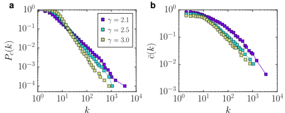
2.3. TheH2model 25 100 ₁₀1 ₁₀2 ₁₀3 ₁₀4 k 10−4 10−3 10−2 10−1 100 Pc (k ) a γ = 2.1 γ = 2.5 γ = 3.0 100 ₁₀1 ₁₀2 ₁₀3 ₁₀4 k 10−3 10−2 10−1 100 ¯c( k ) b

Figure 2.2: Topological properties of synthetic networks. The plots show the topological properties of three networks with N = 104nodes, 〈k〉 = 10 and

differ-ent power-law degree-distribution expondiffer-ents generated with theS1model with

β = 2.5. a, Complementary cumulative degree distributions. b, Clustering

spec-tra. Notice that all three networks exhibit a high average clustering coefficient (higher than 0.5 in all cases).

2.3 The

H

model

In the S1 model, geometry explicitly represents resemblance between nodes,

while the popularity dimension is encoded into the non-geometric hidden de-grees. However, the disentanglement of popularity from geometry is only ap-parent; this is implied by the fact that the model is isomorphic to a different geo-metric model, theH2, in which the geometry of the space encodes both dimen-sions, popularity and similarity, and where the connection probability becomes a function of the distance in the space only [93,94,35,155,2,4]. In this section, we show how to construct a purely geometric representation from theS1model, which defines theH2model, and its connection to hyperbolic geometry.

2.3.1 Isomorphism between the

S

and the

H

models

Consider some given realization of theS1model. We can assign a new hidden

variable ri to every node as a function of its hidden degreeκi according to

ri= ˆR − 2ln

κi

κ0

, (2.6)

whereκ0is the smallest hidden degree in the system and ˆ

R = 2ln N

µπκ2

0

In terms of these new quantities, the connection probability in Eq. (2.1) becomes p µ_R∆θ i j µκiκj ¶ = p³e12(xi j− ˆR)´_{, (2.8)}

where the only pairwise-dependent term is

xi j= ri+ rj+ 2 ln

∆θi j

2 . (2.9)

Strikingly, hyperbolic geometry emerges from this relations; the expression in Eq. (2.9) is, approximately, the distance between two points with radial coordi-nates ri and rj and angular separation∆θi j in the hyperbolic plane with

curva-ture K = −1 (in its native representation), the exact expression for which is given by the hyperbolic law of cosines [94,7],

ˆ

di j= acosh¡coshricosh rj− sinhrisinh rjcos∆θi j¢ . (2.10)

In other words, by mapping every node’s hidden degree onto a radial coordinate according to Eqs. (2.6) and (2.7), all nodes lay on a disk of radius ˆR and their

connection probabilities only depend on the hyperbolic distances separating them (see Fig.2.1). This is, fundamentally, theH2model [94], and Eqs. (2.6) and (2.7) constitute the quasi-isomorphism (the “quasi” here stands for the fact that Eq. (2.9) is not exactly equal to Eq. (2.10)1) between this model and theS1[152], which we will invoke repeatedly throughout this thesis.

2.3.2 Specifications

TheH2model [94] generates realistic complex networks by scattering N nodes on a hyperbolic disk of finite radius ˆR with quasi-uniform density. The density

of nodes is not completely uniform in hyperbolic space, but it is given a radial dependence in order to tune the level of degree heterogeneity in the resulting graph. Indeed, according to Eq. (2.6), a power-law hidden-degree distribution implies an exponential distribution of radial coordinates. Therefore, the radial density is chosen to be

ρ(r ) = α sinhαr

coshα ˆR − 1≈ αe

α(r − ˆR)_{, (2.11)}

for which the resulting degrees are power-law distributed with exponentγ given

byγ = 2α + 1 if α ≥ 1/2 or γ = 2 otherwise. Once all nodes have been sprinkled,

every pair of nodes is connected with the probability given by Eq. (2.8), where

1_{It is important to mention that the goodness of the approximation increases with the radial} coordinates riand rjof the two nodes [94,7] and, henceforth, with increasing network size N .