GROUND DEFORMATION ANALYSIS IN APENNINE AREAS, SEISMICALLY ACTIVE OR ASEISMIC, USING DATA FROM SAR INTERFEROMETRY AND INTEGRATION OF GEOMORPHOLOGICAL AND STRUCTURAL DATA

UNIVERSITA’ DEGLI STUDI DI NAPOLI “FEDERICO II”

Di.S.T.A.R. - Department of Earth Sciences, Environment

and Resources Sciences

Doctorate School in

GROUND DEFORMATION ANALYSIS IN APENNINE AREAS,

SEISMICALLY ACTIVE OR ASEISMIC, USING DATA FROM SAR

INTERFEROMETRY AND INTEGRATION OF GEOMORPHOLOGICAL AND

STRUCTURAL DATA.

XXXI Cycle

Ph.D. Thesis

student: Sergio Nardò

Advisors

:

Coordinator of Doctorate School:

Prof. Alessandra Ascione

Prof. Maurizio Fedi

Co-Advisor:

Prof. Domenico Calcaterra

Prof. Stefano Mazzoli

2

Summary

Summary ... 2

ABSTRACT ... 4

CHAPTER 1 - INVESTIGATION OF GROUND DEFORMATION ... 7

1. INTRODUCTION ... 7

1.1. Objectives ... 8

1.2. Short Historical Compendium about thesis' topics ... 9

1.3. Previous personal experience with the PS tecnique and the reason why a PhD project about this topic ... 10

CHAPTER 2 - MATERIALS AND METHODS ... 12

2.1 Earth Observation with Synthetic Aperture Radar (SAR) ... 12

2.1.1 Satellite missions ... 12

2.2 Advanced DInSAR techniques ... 15

2.2.1 Potential and limitations of multi-interferogram techniques ... 17

2.2.2 Interferogram stacking techniques ... 18

2.3 PS (Persistent Scatterers)-based or PSI (Persistent Scatterer Interferometry) techniques ... 18

2.3.1 SAR acquisition geometry ... 20

2.4 Extraordinary Plan of Environmental Remote Sensing (PST-A) by Ministry of the Environment and Territory and Sea Protection (MATTM) ... 22

2.5 Basic statistics ... 23

2.6 PSs data mining. How make selection in a large dataset ... 27

2.6.1. PSs Classification using frequency distribution ... 27

2.6.2. PSs mean velocity values spatial clustering ... 29

2.6.2.1 Hot Spot Analysis mapping tool (Getis-Ord Gi*) ... 29

2.6.2.2 Cluster and Outlier Analysis mapping tool (Anselin Local Moran's I) ... 30

2.7 Map interpolation: IDW method ... 31

2.8 Time series ... 32

2.9 Selection, Analysis and Mapping Procedures in the various case studies ... 32

CHAPTER 3 - GEOLOGICAL FRAMEWORK ... 34

3.1 The Apennines tectonic framework ... 34

3.2 Seismotectonic framework of the Apennines ... 38

3.3 Structural setting ... 42

3.3.1 Structure of the Northern Apennines ... 43

3.3.2 Structure of the central Apennines ... 44

3.3.3 Structure of the southern Apennines ... 46

CHAPTER 4 - INVESTIGATION OF POST-SEISMIC GROUND DEFORMATION: THE 1980 IRPINIA EARTHQUAKE CASE STUDY ... 49

4.1 Introduction ... 49

4.2 Geological framework ... 53

3

4.3.1 IDW analysis of “native” PS datasets ... 53

4.3.2 Geospatial analysis: Hot Spot and Cluster and Outlier ... 56

4.4 Discussion and Concluding remarks ... 67

CHAPTER 5 - INVESTIGATION OF PRE-SEISMIC GROUND DEFORMATION IN THE 1997 COLFIORITO EARTHQUAKE ... 70

5.1 Geological framework ... 70

5.2 Seismotectonic and SAR remote sensing background of the 1997 Colfiorito earthquake ... 72

5.3 PSs and time series analysis in Colfiorito earthquake area ... 74

5.4 Discussion and Concluding remarks ... 76

CHAPTER 6 - INVESTIGATION OF PRE-SEISMIC GROUND DEFORMATION IN THE 2009 L'AQUILA EARTHQUAKE ... 77

6.1 Seismotectonic and SAR Remote Sensing background of the 2009 L’Aquila earthquake ... 77

6.2 Materials and method ... 78

6.3 Results ... 80

6.3.1 ERS dataset analysis ... 80

6.3.2 ENVISAT dataset analysis ... 80

6.4 Discussion and concluding remarks ... 83

CHAPTER 7 - INVESTIGATION OF PRE-SEISMIC GROUND DEFORMATION IN THE 2013 LUNIGIANA EARTHQUAKE ... 86

7.1 Geologic and tectonic setting ... 86

7.2 Materials and method ... 88

7.2.1 Time series ... 89

7.3 Discussion and Concluding remarks ... 91

CHAPTER 8 - INVESTIGATION OF A-SEISMIC GROUND DEFORMATION IN THE CAMPANIA PLAIN ... 92

8.1 Introduction ... 92

8.2 Geological framework ... 92

8.2 Geomorphological analysis of the northern sector of the Campana Plain ... 99

8.2.1 The Volturno Plain ... 100

8.2.2 The Cancello Plain ... 102

8.3 PSs vertical Vmean, ground deformation maps of Fiume Volturno Campana Plain ... 103

8.4 ERS Time Series analysis ... 115

8.5 ENVISAT Time Series analysis ... 119

8.6 Discussion ... 122

8.7 Discussion and Concluding remarks ... 125

CHAPTER 9 - CONCLUDING REMARKS ... 126

REFERENCES ... 128

4

ABSTRACT

The core of the study herein has been the analysis of PS-InSAR datasets aimed at providing new constraints to the active tectonics framework, and seismotectonics, of several regions of the Apennines. The analysed Permanent Scatterers datasets result from processing of large amounts of temporally continuous series of radar images acquired with the ERS (1992-2000), ENVISAT (2003-2010) and COSMO SKYMED (2011-2014) satellite missions. Such datasets, which are available in the cartographic website (Geoportale Nazionale) of the Italian Ministry of Environment (MATTM) have been collected through time by the MATTM in the frame of the "Extraordinary Remote Sensing Plan" (Piano Straordinario di Telerilevamento Ambientale, PST-A, law n. 179/2002 - article 27), with the aim of supporting local administrations in the field of environmental policies. The database was realized through three phases: the first one (2008-2009), which involved the interferometric processing of SAR images acquired throughout the country by the ERS1/ERS2 and ENVISAT satellites in both ascending and descending orbits, from 1992 to 2008; the second one (2010-2011) integrated the existing database with the processing of the SAR images acquired by the ENVISAT satellite from 2008 to 2010; the third phase (2013-2015) provided an upgrading and updating of the previously developed database on critical areas, based on StripMap H image acquired with a 16-day recurrence, either in ascending or descending orbit, using the Italian national satellite system, the COSMO SKYMED.

With this study, a massive use of Permanent Scatterer datasets is applied for the first time at assessment of ground deformation of large (hundreds of km2 wide) regions of Italy over the last decades, in order to unravelling their current tectonic behaviour. To date in the field of tectonics – in particular, of earthquake geology - the SAR images have been used essentially through the DinSAR technique (comparison between two images, acquired pre- and post-event) in order to constrain the co- and post-seismic deformation (Massonet et al., 1993; Peltzer et al., 1996, 1998; Stramondo et al., 1999; Atzori et al., 2009; Copley and Reynolds, 2014), while the approach that has been used in the case studies that are the object of the research herein is based on analyses of data that (with the exception of the Lunigiana case study) cover an about 20-year long time window. The opportunity of analysing so long, continuous SAR records has allowed detection of both coseismic displacement of moderate earthquakes (i.e., the M 6.3 2009 L’Aquila earthquake, and the M 5 2013 Lunigiana earthquake), and subdued ground displacements - and acceleration – on time scale ranging from yearly to decades.

The specific approach used in this study rests on a combination of various techniques of analysis and processing of the PS datasets. In general, as the analyses that have been carried out aimed at identifying motion values with wide areal extent, a statistical filtering has been applied to PSs velocity values in order to discard from the initial, “native”, dataset fast-moving PSs that may be associated with the occurrence of local-scale phenomena (e.g., landslides, sediment compaction, water extraction, etc.). Furthermore, an in depth inspection of time series of PSs from all of the investigated areas has been carried out with the aim of identifying changing (LoS-oriented) motion trends over the analysed time windows.

A distinctive feature of this study was the estimation of vertical ground displacements. In fact, while most studies on ground deformation are based on analysis of SAR data recorded along either ascending or descending satellite orbits (thus based on LoS-oriented motions), a specific focus of this study was to obtain - starting from LoS-oriented PS velocity values - displacement values in the vertical plane oriented west-east. In order to evaluate vertical displacements, a geometrical relationship was applied to ascending - descending PSs pairs. As PS from ascending and descending tracks are neither spatially coincident nor synchronous, each image pair was obtained by selecting ascending-descending radar images with a time separation within one month. In the L’Aquila region case study, the combination of data recorded along both the ascending and descending satellite orbits has been crucial to the identification of pre-seismic ground motions, undetected in previous works that – similarly – had addressed assessment of possible pre-seismic satellite-recorded signals.

In the various case studies, different kinds of GIS-aided geostatistical analyses were used to extract and synthesise information on ground deformation through the construction of both raster maps of displacement values for the ascending and descending LoS, respectively, and maps of the vertical (z, up - down) component of the “real” displacement vector.

In the Campania plain case study, the PS-InSAR data analysis and processing have been integrated by detail scale geomorphological-stratigraphical analysis. Results of analyses of the two independent data sets are consistent, and point to tectonically-controlled ground displacements in a large part of the northern part of the study area (Volturno plain) during the 1992-2010 analysed time span. In particular,

5 the integrated data sets show that the boundaries of the area affected by current subsidence follow fault scarps formed in the 39 ka old Campania Ignimbrite, while the horst blocks of such faults are substantially stable (or slightly uplifting) during the analysed time window.

Furthermore, mean rates of current subsidence and long-term (Late Pleistocene to present) mean subsidence rates are comparable, pointing to current vertical displacement assessed through the PS-InSAR data analysis as the expression of the recent tectonics of the analysed sectors of the Campania plain. The Campania plain substantially lacks strong historical seismicity. Such evidence suggests that the detected surface displacements result at least in part from aseismic fault activity.

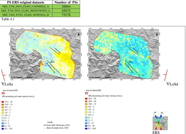
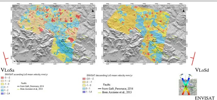
The Monte Marzano case study has allowed assessment of subdued deformation along both the major structures that were activated with the Irpinia 1980 earthquake, i.e. the NE-dipping Monte Marzano fault and the SW-dipping Conza fault, respectively. Ground deformation associated with such structures appears decreasing from the time window covered by the ERS satellites (1992-2000) to that covered by the ENVISAT (2003-2010). These data suggest that post-seismic slip of the M 6.9 has continued until 20 years after the main shock to become very weak in the following ten years. Furthermore, the PS-InSAR data analysis has shown that wide areas located between the Monte Marzano and Conza faults (i.e., in the one that is recognised as the graben structure bounded by those structures) show uplift in the range of 0-2 mm/yr, more evident in the period surveyed by the ERS satellites (1992-2000) and less evident in the 2003-2010 time span (ENVISAT). Such uplift might be related to the occurrence, at depth, of a fluid reservoir that has been independently identified by seismic tomography (Amoroso et al., 2014).

In depth analysis of pre-seismic periods have been carried out in three study areas, i.e. those of the 1997 Colfiorito earthquake, of the 2009 L’Aquila earthquake and of the 2013 Lunigiana earthquake.

The Colfiorito case study has not provided any significant information on possible pre-seismic ground deformation, most probably due to the PS spatial distribution in that region too much discontinuous to allow identification of both net signals from inspection of the rare and sparse PS time series, and statistically meaningful surface displacement patterns.

Both in the L’Aquila and Lunigiana case studies, ground deformation signals in the pre-seismic period have been detected from inspection of PS time series. Pre-seismic ground deformation signals detected in the Lunigiana area (which was affected by a strike-slip faulting earthquake; Eva et al., 2014, Pezzo et al., 2014, Stramondo et al., 2014) are questionable, as they are quite complex and difficult to be interpreted and framed within the local tectonic scenario.

Conversely, very clear and net pre-seismic signals have been identified in the region hit by the L’Aquila normal faulting earthquake. There, in the time span predating of some four years the 6th April 2009 main shock, ground deformation with distinct spatial patterns, and orientations, have been detected. In particular, the PS-InSAR analysis has shown that the hanging wall block of the Paganica fault (the surface expression of the structure activated with the main shock; e.g., Galli et al., 2010) has been subject to slow uplift and eastward horizontal motion from 2005 to September/October 2008, and then (October 2008-March 2009) subject to subsidence and westward oriented horizontal motion. Following coseismic collapse, in the early post-seismic period (April-May 2009), subsidence extended eastwards beyond the Paganica fault trace.

The region affected by opposite pre-seismic motions covers the area in which the 6th April main shock and most of both foreshocks and aftershocks (Valoroso et al., 2013) were recorded, while the inversion of the pre-seismic displacements is coeval with onset of the foreshocks (October 2008; Di Luccio et al., 2010). In addition, such a region includes both topographic highs and lows. All of such features point to a correlation of the detected motions with the seismic phenomena, and suggest a deep-seated causative mechanism, such as volume changes in response to vertical/lateral fluids migration and fracturing processes at depth, with all phenomena having been documented in connection with the 2009 earthquake in the study region (e.g., Di Luccio et al., 2010; Lucente et al., 2010; Moro et al., 2017).

Pre-seismic ground deformation that has been detected in the L’Aquila region could represent a precursor signal of the 2009, M 6.3 earthquake. Such a hypothesis should be tested, in the future, through the continuous monitoring through SAR satellites, but also high-resolution geodetic techniques, of seismically active regions worldwide aimed at detecting the possible occurrence of pre-seismic signals. However, the results of this study point to the long-term (yearly scale) PS-InSAR technique as a tool crucial to the detection of ground deformation in areas struck by recent earthquakes, and to monitoring active – possibly aseismic - structures. Such knowledge may strongly support strategies addressed at territorial planning and mitigation of seismic hazard, and represent an important sustenance for actions ruled by Civil Protection. On the other hand, the results of this study highlight the importance of the existing PS database, and the importance of continuing implementing such an instrument in the future.

7

CHAPTER 1 - INVESTIGATION OF GROUND DEFORMATION

1. INTRODUCTION

Remote sensing data by SAR interferometry (InSAR) provide a one-dimensional measurement of change in distance along the look direction of the radar spacecraft (Line of Sight or LoS) for two orbit geometries, ascending and descending, whose combination results are two - vertical and horizontal - displacement vectors in a vertical plane east-west oriented. Similarity between maps of LoS displacement rate from ascending and descending tracks suggest that the observed displacements may be interpreted as reflecting mostly vertical surface displacement or, conversely, LoS displacements in opposite directions, approaching and moving away from satellite, indicate a horizontal component presence.

Such a technique is largely used to detect and monitor ground deformations induced by landslides, volcanism, tectonics and anthropic processes in urbanized areas (Massonnet et al., 1993; Achache et al., 1995; Carnec et al., 1996; Fruneau et al., 1996; Kimura & Yamaguchi, 2000; Berardino et al., 2002; Corsini et al., 2006; Tizzani et al., 2007; Vilardo et al., 2009, Di Martire et al., 2017).

The development of new techniques, based on the analysis of large datasets and, more in general, the Advanced Differential SAR Interferometry approach (A-DInSAR), has significantly increased the potential of SAR remote sensing for ground deformation detection. The SAR technique has proved to be a powerful tool for exploring the slow motion of the Earth’s surface at local (Ferretti et al., 2000; Prati et al., 2010) and sub-regional scale (Bűrgmann et al., 2006; Corsini et al., 2006; Meisina et al., 2006). The SAR technique has also provided fundamental constraints to modelling of earthquake source mechanisms (e.g., Stramondo et al., 1999; Atzori et al., 2009; D’Agostino et al., 2012; Cheloni et al., 2017). Such a technique is also well suited for the detection of ground deformation possibly predating seismic events, a task crucial to forecasting strategies based on the search for diagnostic precursor signals of severe earthquakes (Jordan et al., 2011). In recent years, research has been pushed forward towards the identification of pre-seismic ground deformation patterns through the use of SAR-based techniques, which are being acknowledged among the most promising tools for the search of earthquake precursors (Moro et al., 2017). Within such a framework, the interferometric Extraordinary Environmental Remote Sensing Plan (PST-A) archive, by Italian Ministry of the Environment (MATTM), retains the millimetre ground deformation data that could be, actually, the most important marker of accumulation of crustal seismogenic stress. Such a dataset may provide fundamental information on the pre-seismic phase of moderate to strong earthquakes that have hit Italy in recent years.

The ground deformation mechanisms that characterize a seismic cycle can provide information about the possible earthquake genetic causes. A great earthquake instantaneously disturbs the existing stress balance within the crust.

Knowledge of how the resultant stress concentrations are relaxed, both temporally and spatially, can that Postseismic transients with durations of a few months to years are seen by Peltzer et al. (1996, 1998) and Savage and Svarc (1997) using Synthetic Aperture Radar (SAR) and Global Positioning System (GPS) data.

Copley and Reynolds, 2014, have measured surface displacements post-seismic signal, from 2 to 16 years following the 1994 Sefidabeh earthquake sequence in east Iran, using Differential Interferometry SAR (DInSAR) data from the ERS and Envisat satellites on descending track only.

Geodetic data spanning the first decades after an event are more likely to provide information about long period relaxation of structures in the crust. The problem is that post-seismic data of this temporal extent are generally unavailable because of the relatively recent advent of sufficiently accurate geodetic measurement

The post-seismic deformation following an earthquake can be measured with terrestrial geodetic stations. Such measurements, in the context of a recurring seismic cycle, actually can be obtained with the dense spatial coverage provided by satellite radar interferometry (Massonnet et al., 1994).

Italy has a medium-high seismic hazard (due to the frequency and intensity of phenomena), very high vulnerability (due to the fragility of building, infrastructural, industrial, production and service assets) and an extremely high exposure (due to population density and its historical, artistic and monumental heritage that is one of its kind in the world). Our peninsula therefore has a high seismic risk, in terms of victims, damage to buildings and direct and indirect costs expected after an earthquake.

In Italy we have numerous studies and documents regarding the seismicity of our peninsula, representing a historic heritage that is without equal worldwide. In the nineteenth century, with the development of seismological sciences, the research into the causes and geographic distribution of earthquakes started to

8 be published. Wider use of seismic instruments from the end of the nineteenth century and monitoring networks in the twentieth century finally provided input for studies into seismic characterisation in Italy. Science today is not yet able to forecast the exact time and place for future earthquakes. The only forecast possible is of a statistical kind, based on knowledge of past seismicity in Italy therefore on the recurrence of earthquakes. We know which areas in the country run a high seismic risk, for earthquake frequency and intensity and therefore where it is most likely that a big seismic event will happen, but it is not possible to exactly determine when it will happen.

Over recent years science has made considerable progress in the study of seismic precursors, in other words the chemical and physical parameters of the ground and underground subject to the variations that can be observed before an earthquake happens. In the future, systematic study of these precursors could allow the initial moment of the earthquake to be fixed, even if false alarms must be avoided, which could prove to be even more harmful.

Research into earthquake precursors has concentrated on:

• Seismological precursors: before a big seismic event a series of microtremors may occur, only detectable by instruments.

• Geophysical precursors: anomalies in the P and S wave speeds, variations in magnetic and electric characteristics of rocks.

• Geochemical precursors: variation in underground waters of the concentration of some chemical elements, in particular of radon, a radioactive gas.

• Geodetic precursors: alterations in the level and slope of ground surface.

Forecasting of earthquakes based on precursors has so far brought disappointing contradictory results. No precursor happens regularly before each important earthquake, for this reason research is moving towards simultaneous observation of different phenomena.

1.1. Objectives

The objectives of the thesis concern the possibility to identify, through the use of more or less recent technologies and techniques of remote sensing (over 20 years of applications), the deformations that the Earth's surface undergoes through the seismic cycles (inter-, pre-, co- and post-seismic) in seismogenic areas and, sometimes, in aseismic ones.

The Ministry of the Environment and Territory and Sea Protection (MATTM), in the context of the Extraordinary Plan of Environmental Remote Sensing (PST-A), have a representative "historical" database of the national territory (see par. 5.), containing the measurements of ground movements obtained by means of SAR interferometry, available through the MATTM National Cartographic Portal (http://www.pcn.minambiente.it/mattm/progetto-pst-prodotti-interferometrici/#9).

The database realization was assigned by the MATTM to the temporary business grouping by e-GEOS S.p.A., as the parent company, and by the Telerilevamento Europa T.R.E. s.r.l and Compulab s.r.l.

The database was obtained by processing ERS 1/2, ENVISAT images, acquired between 1992-2000 and 2003-2010 by ESA, with an almost total coverage of the Italian territory, and very few 2011 - 2014 COSMO SKYMED (ASI) images, all through the multi-interferogram technique.

The Multi-Pass interferometry or A-DInSAR (Advanced Differential SAR Interferometry) techniques are based on radar multi-image analysis. The products of these analyzes derive from complex processing chains of satellite images, called PS (Persistent Scatterers)-based or PSI (Persistent Scatterer Interferometry) techniques.

The PS data, not much used by public administrations, for environmental and territorial control and monitoring, in the scientific field they have been used mainly in the geo-applicative field concerning the issue of hydrogeological risk, for slope gravitational and subsidence phenomena monitoring.

The PS data, unlike the DInSAR, has been not much used in seismological field too.

Therefore, in this thesis they were collected several PS ERS 1/2 and ENVISAT PS dataset, and few COSMO SKYMED ones, over portions of the Apennine chain, and they were subject to post-processing mapping, geostatistical tools, and inspections about the deformation time series.

A very exciting challenge was to investigate if there were, in the "historical" MATTM interferometric database, any "signal" that can reveal the existence of pre-seismic deformation phenomena, that is a geodetic precursors.

9 From what has been said before, as summarized in this paragraph and in the introductory one, areas of interest have been identified for the topics related to post- and pre-seismic ground deformation and ground deformation in almost aseismic areas.

The areas of interest of this PhD project are located in several site of Italian peninsula.

• Monte Marzano, Campania region, 1980, 6.9 Mw Irpinia earthquake - topic objective: post-seismic ground deformation;

• Colfiorito, Umbria region, 1997, 5.7 and 6.0 Mw earthquake - topic objective: pre-seismic ground deformation;

• L'Aquila, Abruzzo region; 2009, 6. Mw earthquake - topic objective: pre-seismic ground deformation;

• Lunigiana, Toscana-Liguria regions boundary, 2013, 5.1 Mw earthquake - topic objective: pre-seismic ground deformation;

• Lower Volturno Plain, Campania region - topic objective: quasi aseismic ground deformation.

1.2. Short Historical Compendium about thesis' topics

The accuracy of the millimetre measurements so far realized by the SAR systems have provided impressive images of surface displacements in areas affected by strong earthquakes, which have contributed to constrain the geometric and kinematic features of earthquake generating faults. As a milestone, Massonet et al., 1993, 25 years ago, published a paper about geodetic data obtained by a space-based technique, the synthetic aperture radar (SAR). They used data from ERS1 ESA satellite to capture the movements produced by the 1992 7.3 Mw Landers earthquake (CA USA). Very impressive remains the "Image of an earthquake" published on 1993 Nature Journal cover (Fig. 1.1). The post-processing interferometric colored fringes, obtained with a pair of ERS1 SAR images, taken just before and little after the earthquake, let's we see and quantify the real areal ground deformation after the main shock. This was/is the differential radar interferometry (DInSAR) technique.

Fig. 1.1. Massonet et al., 1993, "Image of an earthquake"

The DInSAR technique is used nowdays for the identification of surface rupture areas (capable fault is an active fault whose coseismic displacement can intercept the ground surface Vittori et al., 1997; Machette, 2000; Galadini et al., 2012), characterization of the superficial deformation and for the reconstruction of the dynamics of the rupture along the fault plane that gave rise to the main and after shocks.

In the last few years several A-DInSAR multi-interferogram techniques have been developed, including Permanent Scatterers Interferometriy SAR (PSInSAR) by Ferretti et al., 2001 and Small Baseline Subset (SBAS) by Berardino et al., 2002.

10 Vilardo et al., 2009, applied the Permanent Scatterers Synthetic Aperture Radar Interferometry (PS-InSAR, Ferretti et al., 2001) technique to the Campania region (southern Italy), using SAR images acquired in ascending and descending orbits from 1992 to 2001 by the European Remote Sensing satellites (ERS), with the aim to detect ground displacements at a regional scale. The study area, is characterized by intense urbanization, active volcanoes (Phlegraean Fields, Vesuvius and Ischia), seismogenic structures, landslides, hydrogeological instability and includes the southern Apennines chain and Plio-Quaternary structural depressions.

Perrone et al., 2013, used PS-InSAR techniques data to identify areas, in Piemonte region (northern Italy), with similar tectonic deformation rates, mean velocity values (Vmean), operating statistically on a PSs dataset, with help of GIS software, through spatial statistics analysis using a geostatistical analysis tool for PSs data. They derived "isokinematics maps" of the study area.

Costantini et al., 2017, debate how PSI technology is today an operational tool for mapping unstable areas and preventing geo-hazards. Ground deformations due to subsidence, landslides, earthquakes and volcanic activities, and their impact on buildings and infrastructures, can be monitored, even at a national scale. The authors say that many potential final users still ignore the capabilities of Earth observation sensors, and satellite SAR sensors are largely unknown.

Moro et al., 2017, analyzed pre- and post-seismic displacement time series of the PSs and presented evidence of ground deformation preceding the 2009 L’Aquila earthquake, occurred within two Quaternary basins filled with sediments hosting multi-layer aquifers, that are located close to the epicentral area, investigating the seismic cycle associated with the earthquake by applying advanced InSAR techniques to SAR datasets from various satellite missions (RADARSAT-2, ENVISAT and COSMO-SkyMed). The SAR images were processed with the SqueeSARTM, the IPTA and the Persistent Scatterer Pair (PSP) techniques, evolutions of PSInSAR and SBAS ones, which permits estimation of displacement time series for dense sets of locations that correspond to identified persistent scatterers. According to the authors, these techniques are suitable for the identification of earthquake precursors.

1.3. Previous personal experience with the PS tecnique and the reason why a PhD project about

this topic

The 2003 SLAM project (Service for Landslide Monitoring), with some applications in Italy, implemented by the European Space Agency (ESA), use the Permanent Scatterers (PSInSAR) technique (Ferretti et al., 2001), a multi-image advanced differential radar interferometry (DInSAR) technique, for landslide investigations.

In 2006 the Agenzia Regionale per la Protezione dell'Ambiente del Piemonte (ARPA - regional environmental agency) obtained the covering of entire regional territory with interferometric PSInSAR tecnique data, using data from ERS1/2 satellites (1992-2001 time span). In 2010, ARPA Piemonte (regional environmental agency) , in the framework of European Project RISKNAT carried out a study about western Alps using RADARSAT 1 images (2002-2009 time span) processed with the SqueeSAR technique (Ferretti et al., 2011).

The first approaches to the PSInSAR, in Campania territorial administration (Regione Campania), start in 2005 with the TELLUS Project. The writer of this thesis was a component of TELLUS Project team. In the framework of Progetto Operativo per la Difesa del Suolo (PODIS) implemented by national authority of Italian Ministry of Environment (MATTM), TELLUS had the aim to realize an advanced/integrated remote sensing/ground monitoring system mainly dedicated to gravitative ground deformations. In the following years (2007-2009), other types of ground deformations was taken in count (subsidence, tectonic, volcanic) in Vilardo et al., 2009 (where the writer was co-author).

In 2010, the entire experience of PODIS-TELLUS Project with the PSInSAR data sets from 1992 to 2010 from radar spaceborne systems ERS-1/2 SAR (ESA), RADARSAT-1 (Canadian Space Agency), ENVISAT ASAR (ESA), that covered Campania region, was transferred to Regione Campania (Settore Difesa del Suolo).

In that years TELLUS realized some collaboration with Federico II University of Napoli (Prof. D. Calcaterra), about specific geotechnical and geomorphological case studies, making dissemination about PSInSAR.

At the end of 2009 the writer became employed at ARPA Campania that, unlike ARPA Piemonte and other ARPA in northern Italy, did not have a sector dedicated to monitoring peculiar geologic phenomena like landslides, subsidence and ground deformations in general.

11 Despite this, in 2010, the writer published, as ARPA Campania membership, with other authors, the scientific article "L’utilizzo della tecnica PSInSAR™ per l’individuazione ed il monitoraggio di sinkholes in aree urbanizzate della Campania; i casi di Telese Terme (BN) e di Sarno (SA)", in Atti 2° Workshop Internazionale - “I Sinkholes - Gli sprofondamenti catastrofici nell’ambiente naturale ed in quello antropizzato”. ISPRA, Roma, 3-4 Dicembre 2009.

Unfortunately, after this, nothing has changed in ARPA Campania scientific organization. The question that arises is why ARPA Piemonte is monitoring the regional territory with interferometric PSInSAR tecnique while not ARPA Campania?

About at the end of 2015, the writer decides, in order not to disperse the acquired knowledge by TELLUS experience, to participate for XXXI° cycle Earth Sciences Phd selection at Federico II University of Napoli and, after the positve result, he took temporary leave from the ARPA Campania. The project idea was to apply the PSInSAR technique to try to identify some peculiar ground deformation signal in seismogenically active areas possibly comparing them with geomorphological and / or geostructural elements.

In 2016 it was created, by law (L. 132/2016), the Sistema Nazionale di Protezione Ambientale (SNPA) that integrates Istituto Superiore per la Protezione e Ricerca Ambientale (ISPRA national institute) and 21 regional ARPA in a same framework. The purpose of this system is to standardize technical-scientific activities (monitoring and control) throughout the national territory and to produce advanced research in environmental field.

At the end of 2016, it was constituted by ISPRA the Tavolo Nazionale dei Servizi Geologi Operativi (TNSGO) with the objective to promote the PS Journal Italia (operational service for monitoring the movements of the ground based on interferometric data), framed in the strategic plan "Space Economy" promoted by the Italian Presidency of the Council of Ministers and in particular in the Mirror Copernicus program (European Environmental Agency EEA), using requirements provided by Regional Authorities (Environmental Agencies and Geological Surveys).

At the same period too, the Government of the Campania Region has ruled, by law (L.R. 38/2016 and L.R. 10/1998), that ARPA Campania have to monitoring the hazardous and risk area (landslides, sinkholes, subsidence) about natural disasters.

In conclusion, the writer hope is that, when he resume in service, with the additional Phd experience, as well as of TELLUS one, he will find an adequate technical-scientific space in ARPA Campania, to work with the PSInSAR, SQUEESAR or others PS SAR techniques, with the most recent data obtained from the current SAR missions of the Sentinel 1A / 1B (ESA) and Cosmo Skymed (ASI) satellites, in order to comply with a specific legislative provision.

12

CHAPTER 2 - MATERIALS AND METHODS

2.1 Earth Observation with Synthetic Aperture Radar (SAR)

The earth observation through the remote sensing represents today one of the main technical-scientific disciplines that allows to obtain, from an external point of view to the terrestrial system, information, quantitative and qualitative, about areas of interest or specific targets located far from a sensor on satellite platforms, through measurements of an electromagnetic radiation naturally emitted (passive detection) or artificially transmitted and then reflected (active detection), that interacts with the involved surfaces. The passive sensors allow a qualitative observation of an area, working mainly with optical data; in this case the electromagnetic energy is characterized by wavelengths belonging to the visible up to the infrared in the electromagnetic spectrum. The active sensors achieve quantitative information of an observed phenomenon working with wavelengths of the L-, C- or X-band (Fig. 2.1). In particular, radar (RAdio Detection And Ranging) is an active sensors that use electromagnetic waves in the radio wavelengths and determine the distance of an object (registering the two-way travel time of the pulse) and its physical quantities measuring its backscatter intensity.

Fig. 2.1. RADAR wavelengths of the L-, C- or X-band

The limitation of physical antenna aperture was overcome through Synthetic Aperture Radar where signal processing is used to improve the resolution beyond (Curlander et. al., 1991). In others words, SAR “synthesizes” a very long antenna playing on the forward motion of the physical antenna.

These instruments, using microwaves, do not feel the effect of clouds and could achieve measures 24 hours a day obtaining radar images of wide areas.

Radar images are pixels matrixes and each of them it is associated a value of the phase and the amplitude relative to the wave emitted by the antenna and backscattered from the targets.

With two radar images referred to the same area, acquired with temporal and spatial baseline (at different times and in different orbit positions), it is possible to obtain, through a conventional technique called the DInSAR (Differential SAR Interferometry), a new image in which each pixel is associated to the difference of the phases. This image is called interferograms and the phase difference, pixel to pixel, between two SAR images is called the interferometric phase. It contains various contributions among which, the electromagnetic noise, the atmospheric features, the topography of the observed scene, and the possible soil deformation occurred in the interval of time between the two acquisitions. Subtracting the noise, atmospheric and topographic components it is possible to estimate that due to the displacement. Therefore, from a processing of the interferometric phase, compared with the ground topography, it is possible to obtain two kinds of results:

- High resolution Digital Elevation Models (DEMs); - Deformation maps characterized by millimetre resolution.

2.1.1 Satellite missions

The satellites operating between 1990 and 2010 used SAR sensors to acquire in C band.

The main civil satellites equipped with SAR sensors in C band, that have surveyed Italian regions in recent past and no more working, was:

• ERS-1 and ERS-2 (ESA). • ENVISAT (ESA). • RADARSAT-1 (CSA).

13 Furthermore, the SAR sensors in C band currently working are:

• RADARSAT-2 (CSA).

• SENTINEL-1A and SENTINEL-1B (ESA).

The ESA's European Remote Sensing (ERS) satellites have been installed with SAR radar sensors with frequency of 5.3 GHz and wavelength λ = 5.66 cm. Their orbits (Fig. 2.2) are heliosynchronous and slightly inclined to the meridians (8.5 °) and illuminate, from the altitude of 785 km, a strip of territory (swath) approximately 100 km wide. The sensor-target direction or Line of Sight (LOS) is perpendicular to the orbit of the satellite and is inclined on average by an angle equal to 23 ° (θ, off-nadir) with respect to the vertical (Fig. 2.2) .The resolution is about 4 meters in azimuth and 8 meters in the direction of the range (the ground resolution is about 20 m.) The same nominal orbit is traced every 35 days and in a time of about 100 minutes.

The ERS-1 satellite acquired data from the end of 1991 to March 2000. From November 1993 to April 1995, the acquisitions were characterized by particular phases lasting a few months each, in which the acquisition parameters were modified for particular applications. and for acquisition in specific areas of the Earth, including the oceans and poles.

The ERS-2 satellite has been operational since the beginning of 1995 and, until the end of the ERS-1 mission, has performed a scan of the same scene but from a slightly different shooting point and one day after the passage of ERS-1. Thanks to this feature, ESA has guaranteed the availability of Tandem pairs from March 1995 to March 2000, through which it is possible to generate high resolution DEMs exploiting the spatial baseline of image pairs.

Fig. 2.2 Orbit and look features

The ESA satellite ENVISAT (ENVIronmental SATellite), launched in November 2002, replaced and expanded the functions of the ERS-1 and ERS-2 satellites. It is equipped with an ASAR sensor (Advanced Synthetic Aperture Radar), which represented an evolution of the SAR and used a series of antennas that could work with different polarizations and 7 different angles of incidence (between 15° and 45 °) with consequent variation of the scene size observed in a single image. The satellite traveled through a helio-synchronous orbit with a retransmission time equal to that of the ERS satellites (35 days). The instrument acquires in C band (frequency of 5.331 GHz and wavelength of 5.63 cm) but with a slight shift in frequency with respect to ERS-1 and ERS-2 which makes it difficult but possible, through some technical devices, the combination of its data with ERS data to perform interferometric processing. The RADARSAT-1 satellite of the Canadian Space Agency (CSA), launched in November 1995, used a sensor SAR in C band. The observation geometry is a lot flexible, in fact, the angles of incidence vary from 10° to 60°, the radar wave beam can be oriented and the width of the imaging bands can be varied

14 from 45 to 510 km wide, with resolutions respectively from 8 to 100 meters. The cycle repetition of the satellite's orbit was 24 days.

Unlike other satellites, RADARSAT-1 generally acquires on demand.

Thanks to an agreement between RADARSAT International and TRE (spin-off company of the Politecnico di Milano), from March 2003, images were acquired on Italian territory every 24 days in Standard mode, both along ascending or descending orbits. In addition, satellite acquisitions were requested in Fine Beam mode on some sensitive areas, such as Venice, Turin, Rome, Naples, Ancona and Crotone. Most of the Italian areas are covered by at least 60 RADARSAT-1 images in descending geometry and 60 in ascendant. Thanks to the high number of available acquisitions and the shorter acquisition frequency (24 days) compared to the ERS and ENVISAT satellites (35 days), these images allow a higher accuracy in the measurement of deformations, because they allow to limit the effects for the temporal decorrelation of the radar signal.

In December 2007, the satellite 2 was also launched. The orbit is the same as RADARSAT-1, but it is traversed with a 30-minute delay for interferometer entry during the period when the two satellites are both operational. The mission, ensures all the methods of acquisition of RADARSAT-1, will ensure continuity with the data obtained from the previous satellite. Its news is instead related to the different angles with which the system can work that contain up to a resolution of 3 m, both in range and in azimuth, to acquire images from both sides of the platform compared to the direction of flight double-sided imaging ), and to emit and acquire the signal in all polarizations.

Finally, SENTINEL satellites are the last generation of Earth observation sat-ellites of the ESA and the Copernicus group (program of the European Commission). The mission is composed of a constellation of two satellites, sharing the same orbital plane. SENTINEL-1A satellite was launched on April 3, 2014 and SENTINEL-1B on 25 April 2016. The SENTINEL-1 mission includes C-band imaging operating in four exclusive imaging modes with different resolution (down to 5 m) and coverage (up to 400 km). It provides dual polarisation capability, very short revisit times and rapid product delivery. For each observation, precise measurements of spacecraft position and attitude are available. The SENTINEL-1 mission includes C-band imaging operating in four exclusive imaging modes with different resolution (down to 5 m) and coverage (up to 400 km). It provides dual polarisation capability, very short revisit times (12 - 6 days) and rapid product delivery. For each observation, precise measurements of spacecraft position and attitude are available.They provides all-weather, day and night radar imaging for land and ocean services, such as: monitoring of Arctic sea-ice extent, routine sea-ice mapping, sur-veillance of the marine environment, including oil-spill monitoring, monitoring land-surface for mo-tion risks, mapping of forests, water and soil management and to support humanitarian aid and crisis situations.

The satellites operating from 2007, using SAR sensors to acquire in X band, are: • TerraSAR-X (DLR)

• COSMO-SkyMed (ASI)

The TerraSAR-X mission started on June 15, 2007; it is a German SAR satellite mission for scientific and commercial applications. The project is supported by BMBF (German ministry of Ed-ucation and Science) and managed by DLR (German Aerospace Center). The science objectives were to make multi-mode and high-resolution X-band data available for a wide spectrum of scientific ap-plications in fields as hydrology, geology, climatology, oceanography, environmental and disaster monitoring, and cartography (DEM generation). Its main features are: resolution up to 0.25 m (in-staring spotlight mode), an excellent radiometric accuracy, unique agility (rapid switches between imaging modes and polarizations). On June 21, 2010, the twin mission TanDEM-X started, and since then they fly in a close formation at distances of only few hundred meters and record data synchro-nously. This peculiar configuration allows the generation of WorldDEM, which is a DEM of the Earth’s land surface with a vertical accuracy of 2 m (relative) and 10 m (absolute).

COSMO-SkyMed (COnstellation of small Satellites for Mediterranean basin Observation) is a satellite mission ran by the ASI (Italian Space Agency) and the Italian Ministry of Defense. The CSK system is made up of four satellites and it is equipped with High-Resolution SAR, in sun-synchronous polar orbits, phased in the same orbital plane. This results in varied COnstellation of small Satellites for Mediterranean basin Observation) is a satellite mission ran by the ASI (Italian intervals between the satellites along the same ground track of between 1 and 15 days. The first two satellites were launched in 2007, the remaining two in 2008 and 2010, respectively. Its main goal is to provide imagery for environmental monitoring and surveillance applications for the management of exogenous, endogenous and

15

anthropogenic risks, but also commercial products. The CSK system is made up of four satellites and it is equipped with High-Resolution SAR, in sun-synchronous polar orbits, phased in the same orbital plane. This results in varied intervals between the satellites along the same ground track of between 1 and 15 days. The first two satellites were launched in 2007, the remaining two in 2008 and 2010, respectively. Its main goal is to provide imagery for environmental monitoring and surveillance applications for the management of exogenous, endogenous and anthropogenic risks, but also commercial products.

Fig. 2.3 The SAR satellites missions

2.2 Advanced DInSAR techniques

The A-DInSAR (Advanced Differential SAR Interferometry) techniques, o multi-pass interferometry, are based on multi-interferogram or multi-image analysis, that is, they use a long series of radar images related to the same area, from which they come identified some radar targets, which are used to measure displacements.

The multi-interferogram techniques allows to select almost all the SAR images acquired by the selected sensor on the area under examination.

In fact, to implement a multi-interferogram analysis, separate images from very high normal baseline can also be chosen (up to 1200 m with images acquired in C band; Colesanti et al., 2003b), with consequent improvement of the temporal sampling of the phenomena, unlike the differential interferometric technique, for which it is necessary to select only pairs of images characterized by low spatial baseline values (<200-300 m) with the consequent reduction of the sampling frequency.

In other words, while differential interferometry samples the deformation phenomenon under examination through the study of two acquisitions/images (the master, M, and the slave, S), estimating only the cumulative deformation occurred between the two acquisitions or, equivalently, the velocity of linear deformation recorded between them, the multi-interferogram analysis is able to provide the complete description of the temporal evolution of the deformations (Fig. 2.4). Obviously, this capacity is limited by the number and temporal distribution of available acquisitions.

16

Fig. 2.4 Time sampling of a deformation phenomenon obtained by DInSAR analysis and multi-interferogram analysis. As A-DInSAR analyzes guarantee a better temporal sampling of the phenomenon, the movement occurring between the acquisition S5 and S6 can not be measured with the available images (Crosetto et al., 2005b).

The ability of multi-interferogram techniques to describe deformation phenomena, depends temporally on the number and distribution of images available on the study area and, spatially, on the availability of pixels affected by low levels of noise in phase information or pixels characterized by stability in reflection characteristics (Permanent or Persistent Scatterers - PS) during the entire period covered by the acquisitions (Crosetto et al., 2005b).

A-DInSAR techniques can allow to get from a few hundred up to over 1,000 points / km2. We can therefore imagine the grid of radar targets as a dense network of natural GPS stations for monitoring large areas of interest, with a frequency of data updating equal to that of image acquisition (usually monthly or less) and with a spatial density of extremely high measurement points.

The A-DInSAR analysis yelds a database of radar targets for which the following information is generally extracted (Fig. 2.5):

Fig. 2.5 Example of A - DInSAR database

- target position: geographical coordinates (E, N, precision up to ± 2-6 m) and altitude (accuracy up to ± 1.5-2 m);

- average annual deformation speed (mm / year), with precision up to 0.1 mm / year (depends on the distance of the targets from the reference point);

- deformation time series with a measuring frequency equal to that of the review time of the used satellite, and with precision up to 1 mm on the single measurement;

- quality parameters, e.g. standard deviation associated with the estimate of the annual average velocity and coherence of each target.

The coherence provides a measure of the quality of the PS, and quantifies the correspondence of the behavior of the target with the deformation model used in the analysis (typically linear). The coherence

17 can assume values between 0 and 1, or respectively between the total absence of correspondence between the data and the model and their complete agreement. During processing, only radar targets that have consistency greater than a certain threshold are selected. This threshold value is established according to the number of images used for processing (they are inversely proportional) and so that the probability of error in the identification of the targets is contained (i.e. less than 10-5; TRE, 2008b ).

All ground-deformation measurements derived from multi-interferometric analysis are detected along the sensor-target line (Line of Sight - LoS), and they are relative type in both space and time. The deformations are calculated with respect to the position of a reference point on the ground of known coordinates, supposedly fixed or expressly indicated by GPS measurements or optical leveling, and with respect to a reference image chosen within the dataset used for analysis. The displacement measured at each reading (SAR acquisition) therefore represents the difference between the ground altitude at the reading and that at the time of the reference acquisition (zero displacement).

In the last few years several A-DInSAR multi-interferogram techniques have been developed, including: - PSInSAR (Permanent Scatterers Interferometriy SAR) by Ferretti et al., 2001, TRE Milan Polytechnic spin off;

- SBAS (Small Baseline Subset) Berardino et al., 2002, CNR-IREA of Naples;

- IPTA (Interferometric Point Target Analysis) by Werner et al., 2003, Remote Sensing GAMMA, Switzerland;

- CPT (Coherent Pixel Technique) by Mora et al., 2003, Barcelona Polytechnic of Catalonia; - SPN (Stable Point Network) by Arnaud et al., 2003, Altamira Information, Barcelona.

- StaMPS (Stanford Method for Persistent Scatterers) by Hooper et al., 2004, University of Standford; - PSP-DIFSAR (Persistent Scatterers Pairs - DIFSAR) by Constantini et al., 2008, e-GEOS, Rome; - SqueeSAR by Ferretti et al., 2011, Altamira Information TRE.

The ground deformations over time are generally modeled by linear functions and, in other cases, more complex models are adopted, such as quadratic, sinusoidal (seasonal) functions or combinations.

The multi-interferometric techniques are distinguished according to the processing approach in the following two categories (Wasowski et al., 2007): PS (Persistent Scatterers) -based or PSI (Persistent Scatterer Interferometry), and interferogram stacking.

2.2.1 Potential and limitations of multi-interferogram techniques

As first, they do not require any intervention on the ground and make it possible to study large portions of land or areas that are difficult to access, with a consequent reduction in the time and costs of large-scale investigation. They also allow the analysis of phenomena that took place in the recent past thanks to the availability of SAR image archives established in recent years by the various space agencies (ERS archives (1992-2001) and ENVISAT (2002-2010) of ESA and RADARSAT-1 archive (2003-2008) of the CSA, and allow to study phenomena whose velocities are extremely reduced (mm / year) and for which conventional techniques would require years before they can provide meaningful measures.

The multi-interferogram approaches allow to monitor the soil deformations with high precision on the deformation trend (precision in the estimation of the average speed up to 0.1 mm/year, on the single measurement vertical displacement up to 1 mm and E-W displacement up to 1 cm).

In areas of high urbanization, the spatial density of radar targets reaches very high values, up to 400-700 PS/km2, but also over 1,000 PS/km2 with data from high resolution sensors, as Cosmo Skymed or TerraSAR-X. This spatial density of benchmarks is several orders of magnitude higher than that obtainable with conventional geodetic networks and provides higher precision (millimetric) than the GPS (centimeter) analysis in the calculation of vertical displacements.

In addition, radar targets are already present on the ground and, unlike the traditional measuring instruments (geodetic benchmarks, GPS, inclinometers), they do not require any installation or maintenance by operators. However, these approaches do not represent a substitute for other monitoring techniques, but are in complete synergy with them. The integration of multi-interferometric data with traditional geodetic measurements and GPS (Table 2.1), allows in fact to exploit all their advantages and obtain a more complete view on the evolution of the phenomena studied.

18

Multi-interferometric data GPS measurements

- accurate measurements in the vertical direction - high spatial density

- monthly update

- optimization of the positioning of the permanent GPS stations

- displacement measurements along the LoS

- accurate measurements in the horizontal direction - low spatial density

- good time sampling

- removal of systematic errors in the results of the PS technique. Data calibration.

- 3D displacement field

Table 2.1 The characteristics of the multi-interferometric measurements in relation to those of the GPS measurements, show that the two techniques are complementary (TRE, 2008a).

2.2.2 Interferogram stacking techniques

The interferogram stackingtechniques are based on the combination of phase information deriving from the analysis of interferograms generated by the combination of all the acquisitions available on the area of interest (multiple masters) characterized by low baseline values spatial (e.g. <200-300 m). In contrast to the PSI techniques, these approaches exploit the signals deriving from the integration of several adjacent cells and through a multi-looking complex operation they combine and connect the time series of the phase values related to the deformations of the investigated surface. These techniques reduce the effects of decorrelation, maximizing the number of pixels used for the combination of phase contributions and consequently improving the signal to noise ratio, SNR (Signal-to-Noise Ratio). Examples of techniques belonging to this category are the SBAS and the CPT (Fig. 2.6).

Fig. 2.6 Representative scheme of PSInSAR processing

2.3 PS (Persistent Scatterers)-based or PSI (Persistent Scatterer Interferometry) techniques

The radar targets (PS or PSI), used as benchmarks for the measurement of deformations, are immune to the effects of decorrelation, i.e. they maintain the same electromagnetic characteristics (reflectivity) in all the images, varying both the acquisition geometry and the climatic conditions, thus preserving the information of phase in time. The PSs generally correspond both to structures of anthropic origin, such as buildings, monuments, metal structures, dams, viaducts, poles, antennas, and to stable natural reflectors such as exposed rocks (Fig. 2.7).

Fig. 2.7 -RADAR targets on groun surface (from TRE, 2008b).

The techniques belonging to this category are the PSInSAR, IPTA, PSP-DIFSAR, StaMPS and SPN. Generally, processing is performed on datastacks composed of at least 30 SAR images acquired along the same nominal orbit and with the same acquisition geometry (Fig. 2.8). However, the number of acquisitions necessary to implement an analysis is related to the characteristics of the area of interest and the type of radar sensor used.

19

Fig. 2.8 - Representative scheme of generic PSI processing

If several SAR acquisitions on the same area are available, the PS grid can be used to discriminate the various phase contributions related to topography, deformation and atmosphere, taking advantage of their different characteristics with respect to time, space and acquisition geometry (Table 2.2). The atmospheric artifact is calculated as the interferometric phase component that is random in time but correlated in space, that is similar in correspondence of points close to each other.

Time Space Acquisition Geometry

(baseline)

deformation correlated variable uncorrelated

topography uncorrelated variable proportional

atmosphere uncorrelated correlated uncorrelated

Table 2.2 Behavior of phase terms due to topography, deformations and atmosphere, against time, space and normal baseline.

Fig. 2.9 Variation of the reflectivity component of the targets which gives rise to temporal decorrelation, variations of the normal baseline which give rise to geometric decorrelation, atmospheric disturbances (from TRE, 2008b).

The factors influencing the precision obtained with the PS technique are (Fig. 2.9):

- number and temporal distribution of the images available on the area of interest (the greater the number of data, the greater the probability of identifying PS, moreover the acquisitions are frequent, the better the estimate of the displacements);

- density of PS;

- uncertainty in the orbital parameters and changes in electromagnetic properties over time;

- atmospheric noise (possible residual errors in case of atmospheric conditions not perfectly simulated); - distance of the PS from the reference point (as for traditional geodetic networks, the precision decreases with increasing distance from the reference point).

The PSI technique can be applied on different scales:

- Local survey, analyzed area of extension from 1 to 100 km2, characterized by a very high degree of detail and with which the density of the points of measure can reach, in urban area, even 1,000 PS / km2.

20 This analysis can be used for monitoring of circumscribed phenomena, such as landslides or sinkholes, for the purpose of urban planning, for the control of extraction basins or plants.

- Regional survey, analyzed area above 50 km2, that it is a very useful operative tool to characterize phenomena of extended deformation. This analysis can be used for monitoring landslides, subsidies, seismic faults, oil or gas fields, storage basins and mines.

- Linear structures survey, such as pipelines (eg methane pipelines, gas pipelines), motorways, railways, etc., by which information is provided on a strip of 1,000 meters wide land around the structure track, as well as information about detail (the historical series of points) for a strip of 250 meters around the track. - Single Building survey provides a targeted and circumscribed analysis of individual buildings in urban areas that refers to a portion of territory equal to 1 km2, for which you want to receive precise information of movement (analysis of individual buildings, of architectural structures) , etc).

2.3.1 SAR acquisition geometry

As mentioned before, the relative displacement measurements is only along the LoS, not in 3D geographic space. The combination of the satellites motion (quasi-polar, ascending and descending, orbits in Fig. 2.10 left) and the Earth rotation, makes it possible to look at the same area of interest from two opposite acquisition geometries. In fact, over the same geographic area, they are processed two distinct PS database, one for ascending and one for descending orbit.

Theorically, considering the satellites moving exactly along meridians, components of the same real ground displacement, in the same ground point (very rare case), contained in a vertical plane E-W oriented, can be measured, with similar or different values, along both the ascending and descending LoS (Fig. 2.10 right),.

In other words, SAR sensors measure only two components along both the LoSs but not real 3D displacement.

Figure 2.10 SAR image acquisition geometry. On the left, the ascending and descending orbit tracks; on the right, looking at the same ground point from two different point of view (from TRE, PSInSAR Handbook)

In fact, the simplified relationships (1) to (4) (Lundgren et al. 2004; Manzo et al., 2006; Lanari et al., 2007; Tofani et al., 2013) link the components measured along the LoSs and the incidence angle (

θ)

(1)

Dz = (D

+ D

)/2cosθ

(2) Deast = (DLoSd - DLosa)/2senθ

(3)

Vz = (V

+ V

)/2cosθ

(4) Veast = (VLoSd - VLosa)/2senθ

Where: Dz is the vertical component of the displacement; Deast is the horizontal component of the displacement; Vz is the vertical component of the mean velocity; Veast is the horizontal component of the Vmean.

21

Fig. 2.11 A: generic case with LoSs measurements not null; B: case with null measurements on LoSa; C: case with null measurements on both the LoSs

In Fig. 2.11A, a real displacement vector (DR) is oriented along a generic plane in the geographic space: the DLoSa, DLoSd measurements and

θ angle, through relationships (1) and (2),

In Fig. 2.11B, DR is oriented along the plane perpendicular to the LoSa; for this reason there is not projection of DR on LoSa, that is DLoSa is null.

In Fig. 2.11C, DR is oriented along N-S direction; for this reason there is not projection of DR on both LoSa and LoSd, that is both DLoSa and DLoSd are null. For this reason, the component N-S of any deformation can not be detected by SAR.

As a generic example, with ERS and ENVISAT satellites, where LoS incidence angle θ = 23°, in Fig. 2.12 is possible to see a quantitative relationship between the real displacement vector (blue arrow) and the components on the ascending LoS (yellow arrow) and descending one (green arrow).

Fig. 2.12

Conventionally, PS that move along the LoS, away from the satellite, are represented with colors from yellow to red while, with colors from light blue to dark blue, are points moving towards the satellite, with green color they are considered stable (Fig. 2.13).

22

2.4 Extraordinary Plan of Environmental Remote Sensing (PST-A) by Ministry of the

Environment and Territory and Sea Protection (MATTM)

The PST-A is an information system. With it a representative database of the national territory was implemented, containing the measurements of the movements of the terrain obtained by means of SAR interferometry.

The database was obtained by processing, through the multi-interferogram technique generically defined as Persistent Scatterers Interferometry (PSI), all the available ERS and Envisat SAR data over Italy, and then at updating the PSI measurement database based on COSMO-SkyMed HIMAGE (stripmap) data stacks (Fig. 2.14). This was the first InSAR project at national scale, and has required the processing of about 20,000 SAR images acquired from 1992 to 2014 over the whole Italian territory (Costantini et al., 2017; Di Martire et al., 2017), with different spatial densities of measurement points on different types of land covers, although not everywherewith all sensors and acquisition geometries. For each measurement point (i.e. for each PS), both the average displacement rate (in mm/year) and the full time series of displacement (in mm), along the satellite line of sight, are provided.

Fig. 2.14 PST-A project by PSI processing of C-band SAR data, ERS-1 and ERS-2 1992–2000 and Envisat 2002–2010, in upper panel and COSMO-SkyMed HIMAGE SAR data stacks (2011–2014), in lower panel, acquired in the two acquisition geometries, ascending and descending (from Costantini et al., 2017).

23 The data are available through the MATTM National Cartographic Portal, a publishing platform compliant with the guidelines of the European Directive INSPIRE for spatial information dissemination (http://www.pcn.minambiente.it/mattm/progetto-pst-prodotti-interferometrici/#9).

For realization assigned by the MATTM to the temporary business grouping by e-GEOS S.p.A., as the parent company, and by the Telerilevamento Europa T.R.E. s.r.l and Compulab s.r.l.

The processing of the PST-A InSAR data, under the coordination of GEOS, was shared between e-GEOS (which processed 70% of COSMOSkyMed and 60% of Envisat data) and TRE (which processed 30% of COSMO-SkyMed, 40% of Envisat, and all ERS data). Each of the companies relied on their own algorithms and processing chains, PSP (Costantini et al., 2008, 2009) by e-GEOS and PSInSAR and SqueeSAR by TRE (Ferretti et al., 2000, 2001, 2011).

A validation of the PSI measurements of the PST-A project vs GNSS measurements was performed by the CIRGEO department of the University of Padua at the end of the first phase of the PST-A project over the sites of Venice and Bologna. In particular, the standard deviation of the difference between the displacement rates determined by the two technologies ranges from a minimum of 0.5 mm/year up to 1 mm/year.

PSI techniques can provide not only a synoptic view of the displacement field affecting the area of interest in the period of time covered by the radar scenes, but also, for each PS, the time series of the displacements at the satellite acquisition dates, characterized by millimetric precision (Fig. 2.15). The deformation time series represent the most advanced PSI product. They provide the deformation history over the observed period and refered to the LoS of the SAR sensor, i.e. the line that connects the sensor and the target, which is fundamental for many applications, e.g. studying the kinematics of a given phenomenon (quiescence, activation, acceleration, etc.).

The interferometric measurements are freely accessible to everybody through the Portal. In addition, public administrations, both at central and at local level, as well as research institutes, universities, etc., can make agreements with the MATTM to download the data.

Fig.2.15 Example of PS datasheet

2.5 Basic statistics

Some basic information on the statistical analysis of data. Data can be distributed (spread out) in different ways. It can be spread out more on the left or more on the right or it can be all jumbled up (Fig. 2.16).

Fig. 2.16

If a variable (X values) can take on any value between two specified values, it is called a continuous variable; otherwise, it is called a discrete variable.

Just like variables, probability distributions can be classified as discrete or continuous.

With a discrete probability distribution, each possible value of the discrete random variable can be associated with a non-zero probability. Thus, a discrete probability distribution can always be presented in tabular form.

24 A continuous probability distribution differs from a discrete probability distribution in several ways. The probability that a continuous random variable will assume a particular value is zero. As a result, a continuous probability distribution cannot be expressed in tabular form. Instead, an equation or formula is used to describe a continuous probability distribution.

Even though the distribution of X values will be discrete, represented by a histogram or bar chart, this distribution can be approximated by a normal distribution, which is continuous.

A continuity correction factor is used when you approximate a discrete probability distribution with a continuous probability distribution.

For example, a binomial distribution can be approximated with a normal distribution (Fig. 2.17).

Fig. 2.17 Approximate a discrete probability distribution with a continuous probability normal distribution.

The normal distribution is a commonly encountered continuous probability distribution. There are many cases where the data tends to be around a central value with no bias left or right, and it gets close to a normal distribution.

The normal distribution is useful because of the central limit theorem. In its most general form it states that averages of samples of observations of random variables become normally distributed when the number of observations is sufficiently large.

The data is normally distributed when the distribution has (Fig. 2.18): • mean = median = mode

• symmetry about the center

• 50% of values less than the mean and 50% greater than the mean

Fig. 2.18 (see text)

There are many different normal distributions (Fig. 2.19), with each one depending on two parameters: the population mean, μ, and the population standard deviation, σ.

The simplest case of the normal curves is called the standard normal distribution and it is a normal distribution with a mean of 0 and a standard deviation equal to 1.

25

Fig. 2.19 Different normal distributions

The standard deviation is a measure of how spread out numbers are. We find that generally (Fig. 2.20):

68% of values are within 1 standard deviation of the mean

95% of values are within 2 standard deviations of the mean

99,7% of values are within 3 standard deviations of the mean

Fig. 2.20 Standard deviations

It is good to know the standard deviation, because we can say that any value is: • likely to be within 1 standard deviation (68 out of 100 should be) • very likely to be within 2 standard deviations (95 out of 100 should be) • almost certainly within 3 standard deviations (99,7 out of 100 should be)

The number of standard deviations from the mean is also called the "Standard Score", "sigma" or "z-score" (Fig. 2.21).