2021-02-16T16:20:59Z
Acceptance in OA@INAF
Analysis of full disc Ca II K spectroheliograms. I. Photometric calibration and
centre-to-limb variation compensation
Title
CHATZISTERGOS, THEODOSIOS; ERMOLLI, Ilaria; Solanki, Sami K.; Krivova, N.
Authors
10.1051/0004-6361/201731511
DOI
http://hdl.handle.net/20.500.12386/30414
Handle
ASTRONOMY & ASTROPHYSICS
Journal
609
Number
April 18, 2018
Analysis of full disc Ca II K spectroheliograms.
I. Photometric calibration and CLV compensation
Theodosios Chatzistergos
1, Ilaria Ermolli
2, Sami K. Solanki
1, 3, Natalie A. Krivova
11 Max-Planck-Institut für Sonnensystemforschung, Justus-von-Liebig-Weg 3, 37077 Göttingen, Germany 2 INAF Osservatorio Astronomico di Roma, Via Frascati 33, 00078 Monte Porzio Catone, Italy
3 School of Space Research, Kyung Hee University, Yongin, Gyeonggi 446-701, Republic of Korea
ABSTRACT
Context. Historical Ca II K spectroheliograms (SHG) are unique in representing long-term variations of the solar chromospheric magnetic field. They usually suffer from numerous problems and lack photometric calibration. Thus accurate processing of these data is required to get meaningful results from their analysis.
Aims. In this paper we present an automatic processing and photometric calibration method that provides precise and consistent results when applied to historical SHG.
Methods. The proposed method is based on the assumption that the centre-to-limb variation of the intensity in quiet Sun regions does not vary with time. We tested the accuracy of the proposed method on various sets of synthetic images that mimic problems encountered in historical observations. We also tested our approach on a large sample of images randomly extracted from seven different SHG archives.
Results. The tests carried out on the synthetic data show that the maximum relative errors of the method are generally < 6.5%, while the average error is < 1%, even if rather poor quality observations are considered. In the absence of strong artefacts the method returns images that differ from the ideal ones by < 2% in any pixel. The method gives consistent values for both plage and network areas. We also show that our method returns consistent results for images from different SHG archives.
Conclusions. Our tests show that the proposed method is more accurate than other methods presented in the literature. Our method can also be applied to process images from photographic archives of solar observations at other wavelengths than Ca II K.
Key words. Sun: activity - Sun: chromosphere - Sun: faculae, plages - Techniques: image processing
1. Introduction
The Sun’s magnetic field is concentrated into strong-field elements, or flux tubes, in addition to a weaker, more tur-bulent background. The strong-field component is thought to be mainly responsible for solar activity. In the lower solar atmosphere, this strong-field flux manifests itself as dark features, such as sunspots and pores, as well as bright structures forming faculae (or plage) and the net-work. With modern magnetographs and spectropolarime-ters both components can be reliably observed. However, before Kitt Peak National Observatory started recording magnetograms in 1974, typically only sunspot records are available. This has negative repercussions for a number of research fields. One of these is the solar influence on climate through its variable irradiance (Haigh 2007; Solanki et al. 2013; Ermolli et al. 2013).
Regular space-based measurements have shown that the total solar irradiance (TSI, the spectrally integrated solar radiative flux at the top of the Earth’s atmosphere at the mean distance of one astronomical unit) varies on different time scales, from minutes to decades (Fröhlich 2013; Kopp 2016). The variability at time scales greater than a day is attributed to changes in the surface distribution of the
Send offprint requests to: Theodosios Chatzistergos e-mail: [email protected]
solar magnetic field. Models have been developed to recon-struct the solar irradiance by accounting for the competing contributions from dark and bright magnetic features on the solar surface. These models have been successful in re-producing the measured TSI (Krivova et al. 2003; Ermolli et al. 2011; Ball et al. 2012; Chapman et al. 2013; Yeo et al. 2014). However, full-disc images of the Sun, typically used by such models, are only available for the last few decades. Reconstructions of past irradiance changes usually rely on observations of sunspots (Lean et al. 1995; Solanki & Fligge 2000; Wang et al. 2005; Krivova et al. 2007, 2010; Dasi-Espuig et al. 2014, 2016), or concentrations of cosmogenic radionuclides, e.g. 14C and 10Be, (Steinhilber et al. 2009;
Delaygue & Bard 2011; Shapiro et al. 2011; Vieira et al. 2011). However, such data provide information about the bright regions only indirectly and on the basis of strong assumptions.
The time-series of available bright magnetic feature data can be potentially extended with the help of daily full-disc Ca II K spectroheliograms (SHG, hereafter) that have been stored in photographic archives at various sites since the beginning of the 20th century. Indeed, owing to the rela-tion between the Ca II K brightness and the magnetic field strength averaged over a pixel (e.g. Babcock & Babcock 1955; Skumanich et al. 1975; Schrijver et al. 1989; Harvey & White 1999; Loukitcheva et al. 2009; Kahil et al. 2017),
the SHG can be used to describe the temporal and spatial evolution of the solar surface magnetic field, and specif-ically its bright component as seen in the chromosphere. Since SHG allow direct measurements of the surface cov-erage and, with a proper calibration, also the photometric properties of bright magnetic features, the historical pho-tographic archives are an important resource for studies of solar magnetism over the last century and the activity and irradiance variations it produced. This has led to an in-creasing interest towards the recovery and preservation of these early observations, which has recently prompted the digitization of various SHG archives, such as those at the Arcetri (Ermolli et al. 2009a), Coimbra (Garcia et al. 2011), Kodaikanal (Priyal et al. 2013), Meudon (Mein & Ribes 1990), Mitaka (Hanaoka 2013), and Mt Wilson (Bertello et al. 2010) observatories.
Figure 1 presents typical examples of the images derived from the digitisation of SHG (hereafter referred to as digi-tised images). These images show non-uniformity across the field-of-view of solar and non-solar origin, as well as (non-solar) spots and scratches on the photographic support.
Fig. 1. Examples of digitised SHG taken at the: (a)) Arcetri (06/09/1957), (b)) Kodaikanal (14/09/1912), (c)) Mi-taka (25/01/1959), and (d)) Mt Wilson (01/01/1969) observa-tories.
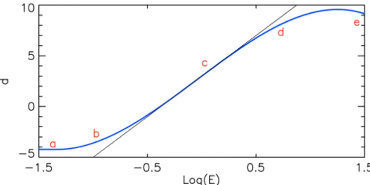
Analysis of SHG requires accounting for these non-uniformities and for the non-linear relation between the blackening of the photographic support (either glass plate or film, hereafter referred to as plate) and the flux of inci-dent solar radiation during the plate’s exposure. This rela-tion is expressed by the characteristic curve (or Hurter and Driffield curve, CC hereafter), which is specific of each pho-tographic observation (Dainty & Shaw 1974) as it depends on a variety of factors, e.g. the exposure time, the gelatine of the photographic plate, the composition of the developers (reducing and fixing baths), the duration of plate develop-ment and the temperature, and degree of stirring during this step. The CC has in general a sigmoid shape. A
typi-Fig. 2. Typical form of a characteristic curve (blue). The labels on the curve denote the different exposure regions: (a) fog level, (b) under-exposure, (c) proper exposure, (d) over-exposure, (e) solarisation. The black line has the same slope as the region of proper exposure.
cal example of a CC is shown in Fig. 2 (see e.g. Sect. 3 or Dainty & Shaw 1974, for more details).
Until recent times, the CC was mainly derived using specific exposures (step-wedges, hereafter) acquired with known relative intensity ratios, in addition to the archived observation (e.g. Fredga 1971; Kariyappa & Sivaraman 1994; Kariyappa & Pap 1996; Worden et al. 1998a; Giorgi et al. 2005; Ermolli et al. 2009a). However, in most cases acquisition of these exposures started many years after the start of solar observations. For example, synoptic SHG were taken regularly since 1915 at the Mt Wilson Observatory, but calibration exposures were imprinted on the plates only from 1961 onwards; at the Kodaikanal site observations started in late 1904 and step-wedges measurements in 1958. Therefore, the bulk of these data lacks specific information on the photometric calibration.
Nevertheless, there have been attempts to calibrate the data lacking wedges. Priyal et al. (2013) calibrated Ko-daikanal data by applying an average CC derived from the available step-wedge exposures on all images. Ermolli et al. (2009b) applied the method presented by Mickaelian et al. (2007) for calibration of photographic plates of star surveys, which is based on information stored in the unexposed and darker parts of the plate. Tlatov et al. (2009) suggested to calibrate SHG by using a linear relation between a stan-dardized centre-to-limb variation (CLV, hereafter) profile published by Pierce & Slaughter (1977) (derived with a 2nd degree polynomial fit and corresponding to 390.928 nm) and the values on the analysed image at two positions.
Various methods have also been used to process Ca II K images and compensate them for the CLV. Some examples are computations that result in radially symmetric back-grounds (Brandt & Steinegger 1998; Walton et al. 1998; Johannesson et al. 1998; Denker et al. 1999; Zharkova et al. 2003), application of a median filter (Lefebvre et al. 2005; Bertello et al. 2010; Chatterjee et al. 2016), 2D polynomial fittings to the entire image (Worden et al. 1998b; Caccin et al. 1998), or interpolation of the mode pixel values within radial and azimuthal disc sectors (Tlatov et al. 2009). How-ever, all of these methods are unable to thoroughly account for the artefacts affecting historical data. Worden et al. (1998a) presented a method that is able to account for the inhomogeneities in the images by fitting a 1D 5th degree polynomial along image rows and columns to density values of the original observation and on the image resulting from
its 45◦rotation. Regions with values outside the ±2σ inter-val of the image, where σ is the standard deviation, were excluded from the analysis and the background is estimated by applying a median, low-pass filter to the average of the fit. Other studies applied variations and combinations of methods previously described in the literature (e.g. Ermolli et al. 2009b; Singh et al. 2012; Priyal et al. 2013). For in-stance, Priyal et al. (2013) used the method of Denker et al. (1999) and a modified version of the approach suggested by Worden et al. (1998a), applying a 3rd degree polynomial fit instead of the originally proposed 5th degree polynomial.
The long list of references above show that many meth-ods have been employed for processing and calibrating his-torical Ca II K observations. However, their aptness and accuracy has generally been discussed only qualitatively.
In this paper we present a new method to calibrate the historical photographic Ca II K SHG as well as a novel method to compensate for various patterns on the data. These patterns include the CLV of the solar intensity and patterns of non-solar origin introduced by observational and archival processes. This method, which works without knowledge of the specific CC of the analysed plate and in the absence of step-wedge imprints, is based on the com-putation of the CLV of density values on quiet Sun (QS, hereafter) regions. Importantly, we rigorously test our tech-nique against modern CCD-based data artificially degraded to correspond to photographically obtained SHG.
The historical and modern observations used in this study are described in Sect. 2. The method is presented in Sect. 3. We assess the accuracy of the method with syn-thetic data that have known characteristics and artefacts and test the proposed method on a large sample of SHG in Sect. 4. We compare our method with other approaches pre-sented in the literature in Sect. 5 and draw our conclusions in Sect. 6.
2. Observational data
The historical observations, on which our technique is tested, are the digitised SHG from the Arcetri (Ar), Coim-bra (Co), Kodaikanal (Ko), Meudon (Me), Mitaka (Mi), McMath-Hulbert (MM), and Mt Wilson (MW) observa-tories. These images were taken in the Ca II K line at λ = 393.367 nm, with nominal bandwidths ranging from 0.01 nm to 0.05 nm and scanning time of several minutes needed to cover the solar disc. The data, which were taken between February 1907 and May 2002 with different instru-mental set-ups and stored mainly on photographic plates, were digitized by using various devices and methods. This results in solar images with different sizes and characteris-tics depending on the archive.
The modern observations used to test our technique were taken at the INAF Osservatorio Astronomico di Roma (OAR) with the Precision Solar Photometric Telescope (Rome/PSPT, Ermolli et al. 1998, 2007). These data were acquired from August 2000 to October 2014, by using an interference filter centred at the Ca II K line with a 0.25 nm bandwidth and the exposure time much shorter than for the historical observations, usually about 0.06 s. We anal-ysed images after the usual reduction steps (dark current removal and flat fielding) that greatly reduce instrumental effects and after they were resized to half their original di-mension (2 arcsec per pixel after resizing), to roughly match the size of the historical data.
Key information about the datasets used in this study is summarised in Table 1.
The available data include estimates of the solar radius R and centre coordinates in the images. To avoid our results being affected by any uncertainties in the radius estimates, we only analysed the disc pixels within 0.99R (0.98R for Ko). This corresponds to µ = cos θ = 0.14 (µ = 0.2 for Ko), where θ is the heliocentric angle.
3. Method description
The digitized SHG reflect the blackening degree of the emul-sion, which is proportional to the transparency T of the plate and is related to the density d of the photographic emulsion since:
d = log (1/T ). (1)
The modern data represent the flux of incident radiation during the observation. The CC is defined as the relation d = f (log E) (shown in Fig. 2), where E = I × t is the plate exposure, I the incident energy per unit area and t the exposure time. Assuming that the plate was exposed evenly, the CC becomes d = f (log I). Therefore the photometric calibration of the data means applying on them the specific and appropriate relation between d and I.
Our method of calibration and processing of the SHG is based on the assumption that, in these observations, the CLV of intensity in the internetwork regions, i.e. the qui-etest part of the QS, does not vary with time, in agree-ment with White & Livingston (1978, 1981), Livingston & Wallace (2003), and Livingston et al. (2007). This assump-tion is also supported by the results of Bühler et al. (2013) and Lites et al. (2014) that the internetwork magnetic flux, which is the main component of magnetic field populating these quietest parts of the solar surface, remains unchanged over the solar cycle. Before applying the proposed method to the historical images, we convert their values to densi-ties according to Eq. 1. Figure 3a) shows the density image corresponding to the Ko observation displayed in Fig. 1b). The main steps of our method can be summarised as: – Calculation of the 2D map of QS regions in each image
(including CLV and inhomogeneities);
– Extraction of the 1D QS CLV profile in each image; – Construction of CC by relating the 1D QS CLV to a
reference 1D radial intensity QS CLV from CCD-based Rome/PSPT observations;
– Calibration of the image using the CC; – Compensation for the intensity CLV.
Visual inspection of historical data shows QS density patterns (2D QS background, hereafter) that are in general strongly non-symmetric and inhomogeneous (see, e.g., Fig. 1). This is due to a plethora of problems affecting the data, introduced either during the observation (e.g. partial cov-erage by clouds, vignetting, uneven movement of the slit), the development (e.g. non homogeneous bathing, touching the plate before the process was finished), the storage pe-riod (e.g. dust accumulation, scratches, humidity, ageing burns), or the digitization (e.g. dust, hair, loss of dynamic range) of the plate. Since results from modern observations indicate the radial uniformity of radiative emission of the internetwork (1D radial QS, Livingston & Sheeley 2008; Peck & Rast 2015), we assume that all departures of the
Table 1. List of Ca II K digitised image archives considered in our study.
Observatory Years Number of images Spectral width Disc size Data type Pixel scale Reference
[nm] [mm] [bit] [”/pixel] Arcetri 1931 − 1974 5141 0.03 65 16 2.4 1 Coimbra 1994 − 1996 79 0.016 87 16 1.8 2 Kodaikanala 1907 − 1999 22164 0.05 60 8 1.3 3 Meudon 1980 − 2002 5727 0.015 86 16 1.5 4 Mitaka 1917 − 1974 8585 0.05 variable 16, 8b 0.9, 2.9b 5 McMath-Hulbert 1942 − 1979 5593 0.01 17.3 8 3 6 Mt Wilson 1915 − 1985 36147 0.02 50 16 2.7 7 Rome/PSPT 2000 − 2014 2000 0.25 ∼ 27 16 2c 8
Notes. Columns are: name of the observatory, period of observations, number of images, spectral width of the spectrograph/filter, the size of the solar disc on the plate, digitisation depth, pixel scale of the digitised file, and the bibliography entry.(a)These data have more recently been re-digitised with 16-bit data type extending the dataset from 1904 to 2007 (Priyal et al. 2013; Chatterjee et al. 2016).(b)The two values correspond to the period before and after 02/03/1960, when the images were stored on photographic
plates and on 24x35 mm sheet film, respectively.(c) The pixel scale is for the resized images.
References. (1) Ermolli et al. (2009a); (2) Garcia et al. (2011); (3) Makarov et al. (2004); (4) Mein & Ribes (1990); (5) Hanaoka (2013); (6) Fredga (1971); (7) Bertello et al. (2010); (8) Ermolli et al. (2007).
2D internetwork map in SHG from a radially symmetric map are image artefacts of non-solar origin.
It is worth mentioning that the bandwidths listed in Table 1 are nominal, while the real values can vary even within a single SHG. The varying bandwidths mean that also the heights of the atmosphere that are sampled change. With broader bandwidths, the photospheric contribution is higher and plage regions appear less bright, while sunspots are more visible. As an example, Fig. 4 shows a MW ob-servation where the right part of the image was taken with a broader bandwidth, either intentionally or due to instru-ment problems. If the bandwidth of the observations was varied or if they were centred at a slightly different wave-length this would have resulted in a different limb darkening profile. However, as information on the real bandwidth is not available, in our analysis we have to assume that the bandwidth of the observations has remained constant over the disc and for all data within an archive.
3.1. Background computation
We first derive the 2D QS background. For this, it is essen-tial to accurately exclude active regions (AR, hereafter), otherwise there is a risk of overestimating the background due to the contribution of remaining AR. The process of calculating the 2D QS background can be outlined as fol-lows:
– Get a rough estimate of the background;
– Use the last estimate of the background to identify and exclude AR;
– Iteratively repeat the process of calculating the back-ground and identifying the AR until sufficient accuracy is achieved;
The first rough estimate of the background is obtained in 3 steps.
– Step 1.1. The solar disc is divided into azimuthal slices of 30◦ that cover the disc in steps of 5◦. Within each slice we apply a 5th degree polynomial fit of the form d = f (µ). The best fit values of d are assigned to all pixels within a given slice. Results obtained from contiguous slices are
gradually averaged and stitched together (this method will be referred to as rotating slices).
– Step 1.2. We compute the density contrast image Cd
i =
(di− dQSi )/d QS
i , where di is the original density image and
dQSi the density background resulting from Step 1.1 at the ith pixel.
– Step 1.3. We identify the regions in the density image lying outside 1σ of the result of Step 1.2. These are tenta-tively identified as AR and are excluded from the further analysis (note that the removal of non-AR pixels in this process does not influence the results; it is more important to discard as many AR pixels as possible).
– Step 1.4. We apply a 5th degree polynomial fit to the density image, excluding AR defined in Step 1.3, along each column and row of the image separately (similarly to Wor-den et al. 1998a, but without the 45◦ rotation of the disc). To all pixels of each analysed column/row we assign the density values resulting from the best fit. We get a back-ground map by stitching together the results obtained from the best fit; multiple values derived for the same location on the solar disc are averaged (we will refer to this method as column/row fittings).
The calculations described in Steps 1.1–1.4 provide a first, rough estimate of the background. However, the iden-tification of AR at this stage is rather inaccurate and the obtained values of the background around AR are over-estimated. The varying contrast for different µ positions renders the identification near the limb less accurate.
Therefore in order to improve the AR identification and the calculation of the background, we iteratively repeat the following steps:
– Step 2.1. We compute the density contrast image Cd
i =
(di− dQSi )/d QS
i , where di is the original density image and
dQSi the density background resulting from the previous cal-culation at the ith pixel. During the first iteration dQS is
the rough background estimate (from Step 1.4 ), afterwards we use the result of the previous iteration.
– Step 2.2. We remove the AR in the original density image, retaining only the pixels that fulfil the threshold criteria
Fig. 3. Selected processing steps of Ko observation taken on 14/09/1912: (a)) original density image, (b)) first estimate of background map (after Step 1.4 ), (c)-h)) results of each step of the iterative process (Steps 2.1–2.5 ), (e) and f )) correspond to Step 2.3. The black square in panel f ) shows the dimensions of the window used for the median filter in Step 2.4 (see Sect. 3.1 for details).
Cd
i > hCdi+l1σ or Cid < hCdi−l2σ, where l1,l2 are the
applied thresholds. For the first 3 iterations l1 = 1 and
l2 = 4, afterwards l1 = 0.5 and l2 = 1. These threshold
values were chosen following a series of tests which showed that they effectively removed plage, network and sunspots, leaving just internetwork regions. See discussion in Sect. 4.1.2.
– Step 2.3. To fill in the gaps left by the AR over the whole disc in the original density image we apply the column/row fittings on the image obtained in Step 2.2. To avoid artefacts of the fit at the limb due to missing values, the gaps by the AR in the outer 0.1R are first filled in with the rotating slices method. The column/row fittings method is repeated two more times to the residual of the density image to the calculated background in order to improve the accuracy of the computation (see discussion in Sect. 4.1.2). All three computations are summed together.
– Step 2.4. We apply a running window median filter on the image resulting from Step 2.3. The filter window width used is R/6 (shown with a rectangle in Fig. 3f; see discussion in Sect. 4.1.2). To avoid inconsistencies, the outer R/12 part of the disc is re-sampled outside the disc to fill the space between R and R + R/12 and the pixel values of the re-sampled section are adjusted so that the median filter is not affected by the pixel values outside the disc.
– Step 2.5. We identify dark and bright linear artefacts affecting many of the SHG (for instance see Fig. 1d)) by separately fitting a polynomial to every row and column of the residual image between the original density image and the result of Step 2.4, excluding the AR. The fit is repeated 3 times as in Step 2.3.
The sum of the maps derived in Steps 2.4 and 2.5 is the final background map of each iteration. The five-step
processing described above is repeated until the difference between two subsequent background maps does not improve the accuracy of the QS background further. Usually 4 iter-ations allow lowering the relative unsigned mean difference between maps from two consecutive iterations to < 0.1%.
The result of the processing described so far is usually an asymmetric map (non-symmetric background, NSB here-after) that describes the 2D QS background of the original image. The asymmetry is caused by a residual pattern that includes small- and large- scale inhomogeneities due to im-age problems, e.g. dark and bright bands and linear arte-facts, stray light features, image gradients. Figure 3 shows different steps of the processing on a randomly selected Ko SHG. In particular, the original density image is shown in panel a), the result of the first column/row fittings process in panel b), while panels c)–h) show the results of each step (2.1–2.5) of the iterative process.
Finally, we apply the method of Nesme-Ribes et al. (1996) on the residual image between the original and the NSB to identify and compensate any offset in the average level of the computed NSB and the analysed image. The method by Nesme-Ribes et al. (1996) identifies the level of the QS as the minimum of the average densities of disc re-gions with density values within ±kσ, where k takes values between 0.1 and 3.0.
3.2. CLV extraction
We compute the radially symmetric background (SB here-after), which in turn gives the 1D QS CLV, by applying a 5th degree polynomial fit to the density values d = f (µ) of the deduced NSB. All image pixels are considered and the fit is weighted with the local σ defined within 100 con-centric and equal area annuli. This is the most important
Fig. 4. MW observation taken on 28/06/1979, where the right part of the image was taken with a broader bandwidth than the left part.
step for the calibration process, because the way the 1D QS CLV is defined, it determines the CC.
Our calculation of NSB includes possible vignetting af-fecting the original SHG, however this leads to miscalcu-lation of the 1D QS CLV. Under-exposure depends on the intensity level, while vignetting is a purely geometric ef-fect. Unfortunately, the geometry is such that their effects are similar, and vignetting is known to darken solar obser-vations towards the limb, resembling the effects of under-exposure. The effects of vignetting are expected to be re-stricted mostly at the edges of the image, in which case it might not affect the solar disc at all or it is almost indistin-guishable from under-exposure. Notwithstanding the simi-larities of their effects on the solar observation, some dif-ferences in the signatures of vignetting and under-exposure on the QS CLV and CC exist. In fact, vignetting can po-tentially affect larger parts of the solar observation than under-exposure, by modifying the CLV even near the image centre in contrast to under-exposure that mainly affects ob-servations near the solar limb (see Fig. A.10). This is valid as long as the under-exposure is not extreme. However, in extreme cases the image quality is anyway very poor and such images cannot be processed meaningfully.
We attempt to estimate the vignetting on the anal-ysed image and account for it in the calculation of the 1D QS CLV, by comparing the SB with a rescaled version of the logarithm of the CLV retrieved from the CCD-based Rome/PSPT observations. If there is no vignetting, the SB from the polynomial fit is kept. Otherwise, the SB is com-puted by rescaling the CLV from the modern observations. Its lower values are adjusted so as to find the minimum density for which the difference between SB and the CLV derived with the fit continuously increases towards the limb. 3.3. Photometric calibration
In our approach, we perform the photometric calibration by seeking for information stored on the solar disc that can be used in a similar manner as the often missing calibration wedges.
For each analysed image, we deduce the CC by relating the density values obtained from its SB at a given µ position
to the logarithm of intensity values derived from modern Rome/PSPT observations at the same disc location. The amount of equal area annuli we use to acquire this relation and apply a linear fit to it is equal to the nearest integer of 2R. This is consistent with the assumption that the QS density values in good-quality observations lie on the linear part of the CC. From the fit we only exclude the last value that corresponds to the regions very close to the limb, due to the higher uncertainties that characterise these regions. We linearly extrapolate the computed relation to the whole range of density values on the image and make use of the fit parameters to photometrically calibrate the original density image. The result of this procedure is illustrated in Fig. 5a). We also photometrically calibrate the estimated NSB. Removal of the QS CLV from the calibrated image and normalization to it then provides the contrast image of the analysed SHG (Fig. 5b)).
Figure 6 shows the CC derived from the processing of the Ko observation displayed in Fig. 3a).
Fig. 5. (a) Photometrically calibrated, and (b) contrast image corrected for the CLV for the Ko observation shown in Fig. 3. The colour scale of the calibrated image covers the full range of intensities on the disc, while the contrast image is shown within the intensity range [-1,1].
Fig. 6. Left : CC derived from the processing of the Ko obser-vation shown in Fig. 3 (red), measured CC for the QS (orange) with 1σ uncertainty (black) and the whole background (blue). The slope of the derived CC is also shown. Right : Distribution of density values for the QS (blue), AR (red) and whole disc (black). The horizontal dashed line in both panels denotes the highest value of the QS CLV.
4. Performance of the method
4.1. Synthetic data
We tested the method proposed in Sect. 3 on a large num-ber of synthetic images that were obtained from contrast Rome/PSPT images by imposing on them known radially symmetric CLV and a variety of inhomogeneities identified in historical observations (and converted to intensity). We then converted the degraded images from intensities to densities by applying various CC, thus emulating historical observations. We used the 2000 Rome/PSPT images described in Sect. 2, which were processed as described in Sect. 3.1 to derive contrast images. These contrast images are defined as CI
i = (Ii − I
QS
i )/I
QS
i , where Ii is
the intensity, and IiQS the intensity of the QS of the ith pixel. The imposed CLV are in the form of a 5th degree polynomial function of ln µ, as presented by Pierce & Slaughter (1977), with parameters determined from the Rome/PSPT observations. The range of values of the imposed intensity CLV is [0.6, 1.0], while the contrast range of the facular pattern is [0.1, ∼0.6], and of the network pattern is [0.026, 0.1]. These ranges match the ones found on images of the Ko, Ar and Mi archives.
We produced 8 subsets of synthetic images with the following features:
- Subset 1: Ideal density images with symmetric back-grounds, no linear artefacts or bands, to estimate the precision of the proposed method and the sensitivity of results to the level of solar activity.
- Subset 2: Images with imposed CC that are linear functions with varying slopes, to test the sensitivity of the method to different slopes of CC within the range 0.1 – 4.0.
- Subset 3: Images with imposed CC that are non-linear functions with various levels of over- and under-exposure (shown in Fig. A.5), to estimate errors in the retrieved calibration due to exposure problems.
- Subset 4: Images with different sizes, to test the accuracy of the method on the various datasets. The disc diameter was varied between 200 and 1100 pixels.
- Subset 5: A vignetting function with different strength levels was added to images, to test the ability of the method to identify possible vignetting effect and to distin-guish it from other artefacts. The vignetting used here is axi-symmetric.
- Subset 6: Various large scale density patterns of non-solar origin were imposed (shown in Fig. A.11), to evaluate the efficiency of the method to distinguish between the solar and non-solar patterns and the accuracy of accounting for the latter.
- Subset 7: Images with a different CLV (shown in Fig. A.13) than the one used during the standardization of the CC, to test the errors of calibrating data obtained with different bandwidths.
– Subset 8: A combination of all the artefacts mentioned above was added randomly on each image, to produce an inhomogeneous dataset resembling the historical ones. The CC is defined as a 3rd degree polynomial function with randomly selected parameters within the following ranges: [-4.6, -1.3] for the constant term, [0.5, 4.0] for the linear term, [-0.03, 0.00] for the quadratic term, and [-0.03, 0.00] for the cubic term. The range of intensities within
the undegraded images varies and the logarithm of it lies between -1.2 and 0.5 (similar to those shown with the light grey area in Fig. A.5).
Figures 7 and 8 show some examples of the synthetic images derived from the same contrast Rome/PSPT ob-servation (taken on 21/08/2000), illustrating the variety of problems we aim at addressing with the application of the proposed method on these data. In the same figures we show the results obtained for these synthetic data and the pixel-by-pixel errors in the NSB calculation and the cali-brated contrast images. The contrast images used to derive the errors are offset so that the mean QS contrast value is 1.
4.1.1. Overall performance of our method on synthetic data Table 2 summarises key aspects of the various synthetic datasets, and quantitative results obtained by testing the proposed method on them. The results are briefly presented in the following and are described in greater detail in Ap-pendix A. Table 2 summarizes the results derived from the analysis of all data within the various subsets. An exception is made for subsets 3 and 6, for which the presented val-ues correspond to results restricted to images representative of historical data of reasonable quality, i.e. excluding syn-thetic images made to suffer from extreme exposure prob-lems affecting the QS regions or images with superposed large-scale patterns whose amplitudes were larger than 0.6 of the CLV.
The results obtained for subsets 1–6 show that our method recovers the QS density CLV with average relative error < 3% in the absence of strong non-solar patterns af-fecting the image, and error < 6.5% if the extreme cases of inhomogeneities encompassed in subset 6 are also included. The results derived from subset 7 prove that the above ac-curacy is maintained as long as the CLV differs by roughly < 10% from the one we imposed on the data.
The results obtained from the subset 8 demonstrate that the proposed method retrieves the NSB affecting the obser-vation with a maximum relative error < 2% averaged over all the analysed images. We found that, similarly to arte-facts on the historical images, the presence of gradients on the synthetic images introduces errors in the calculation of SB, which affects the range of values in the calibrated data. Figure 9 illustrates the accuracy of the proposed method on the most challenging subset 8. Shown are the maximum and average values of the relative difference as well as the RMS difference between the calibrated and processed con-trast image and the original undegraded synthetic concon-trast image. Throughout this analysis the relative differences are given in absolute values (unsigned), but we also provide the signed average difference. These values quantify the final errors of our image processing, which is comprised of the photometric calibration and the removal of the CLV and other image patterns from the analysed image and finally provides the corrected contrast image. We found that the maximum differences are on average < 6.5%, while the av-erage differences are < 1%. There is, however, a tail consist-ing of images with higher maximum or average differences. For images representative of low activity periods, maximum errors are approximately 2% lower than those found for im-ages at high activity periods, which illustrates the need for a very careful removal of active areas prior to carrying out
Fig. 7. Examples of the calibration procedure on synthetic images from subsets 1 – 4 (from top to bottom) produced by Rome/PSPT image taken on 21/08/2000. From left to right: (1)) density images, (2)) imposed backgrounds, (3)) calculated backgrounds, (4)) calibrated contrast images, (5)) pixel-by-pixel relative errors in NSB, and (6)) relative errors in calibrated contrast images. Here we show the following cases: subset 2 – CC with slope of 0.1; subset 3 – combination of the strongest under-and over- exposure (case 10 underexposure under-and 10 overexposure in Fig. A.5); subset 4 – disc diameter of 1100 pixels. Also given (below the images in columns 5 and 6) are the values of the RMS, mean, mean absolute and maximum relative differences within the disc up to 0.98R.
any image processing. We discern no significant variation of the mean and RMS differences over the solar cycle.
We also tested the accuracy of our proposed method for studies of variations in the fractional coverage of the solar disc by AR and network. Figure 10 shows the relative dif-ference between the disc fraction of various solar features identified on the processed and unprocessed images of sub-set 8. The disc features were identified by applying a sub-set of constant thresholds on the original (i.e. prior to degra-dation) and final (i.e. after recovery) contrast images. The
thresholds used here were defined on the Rome/PSPT data to describe the plage and network regions. The thresholds in the contrast values used are thp = 0.21 and thn = 0.03
for the plage and network, respectively. Figure 10 demon-strates that the estimated disc fractions for the processed data typically lie within 2% of the values derived from the original data.
Fig. 8. Same as Fig. 7 but for subsets 5 – 8. Here we show the following cases: subset 5 – strongest vignetting (red curve in Fig. A.10); subset 6 – level 5 of inhomogeneity No. 2 (shown in Fig. A.11); subset 7 – CLV No. 4 (shown in Fig. A.13); subset 8 – vignetting No. 2, level 5 of inhomogeneity No. 4, CC d = −3.6 + 3.6 log I − 0.01(log I)2− 0.004(log I)3
, and CLV used d = 1.0 + 0.33 log(µ) + 0.06(log(µ))2− 0.04(log(µ))3− 0.05(log(µ))4− 0.01(log(µ))5
that lies roughly between cases 6 and 7 in Fig. A.13.
4.1.2. Performance on individual steps of the processing Our method includes original ideas for processing SHG (e.g. rotating slices), but it also partly uses ideas from the previ-ously published methods described in Sect. 1. By testing all these methods on synthetic data we identified their draw-backs, which helped us to optimize the steps of the method proposed here.
For example, in our calculation of the background, we do not rotate the image by 45◦as proposed by Worden et al. (1998a). We found that the rotation does not improve the
accuracy of the image processing further, if the outcome of other processing steps has been optimized. In contrast, our iterative fitting improves the accuracy of the AR identifi-cation and, in turn, of the QS estimation as compared to both non-iterative computations with a 5th degree polyno-mial function as suggested by Worden et al. (1998a) and iterative computations with higher degree functions. How-ever, we also noticed that on average more than three com-putations of the fit per iteration step merely results in an increase of the noise of the final NSB map derived from the processing without improving the accuracy of the result.
Table 2. Summary of the characteristics of synthetic data and fidelity of retrieved images.
Subset N Type of CC N CC Inhomogeneities NSB Max [%] Contrast Max [%] Contrast RMS [%]
(1) (2) (3) (4) (5) (6) (7) (8)
mean range mean range mean range
1 500 linear 1 no 1.3 0.8–2.3 2.4 1.5–4.0 0.5 0.3–1.0
2 200 linear 20 no 1.3 0.1–3.1 3.1 1.7–5.2 0.6 0.3–0.8
3 1000 3rd degree 100 no 1.3 0.8–1.8 6.4 1.5–25.1 0.8 0.3–2.4
4 100 linear 1 different disc sizes 1.8 1.0–3.2 2.7 1.8–5.4 0.5 0.3–0.9
5 100 linear 1 vignetting 1.4 0.9–1.8 2.6 1.5–4.0 0.6 0.3–0.8
6 2000 linear 1 NSB 2.9 1.1–11.3 5.1 1.9–32.5 0.9 0.4–5.9
7 100 linear 1 different CLV 1.4 0.9–1.9 9.8 1.6–31.7 2.1 0.3–6.5
8 2000 3rd degree 2000 all 1.8 0.2–18.3 6.5 1.5–29.0 1.2 0.3–6.4
Notes. (1) ID number of the subset, (2) number of images within the subset, (3) type and (4) number of different CC, (5) type of inhomogeneities, (6) relative maximum error in the retrieved NSB, (7) maximum relative and (8) RMS errors of the calibrated contrast images. For (6)–(8) we provide the average and the range of values in percent.
Fig. 9. Left: Relative difference between the calibrated and CLV-corrected image with our method and the original image (within 0.98R) for all the synthetic data of subset 8. RMS dif-ference (green), mean absolute difdif-ference (blue), mean differ-ence (orange) and maximum differdiffer-ence (red). Each of these val-ues refers to a single image at a time (e.g. the difference aver-aged over all pixels, or the maximum value found in one pixel of the image). These differences are plotted vs. the date on which the original Rome/PSPT images (that were randomly distorted) were recorded. Note that the maximum difference values have been divided by 10 to plot them on the same scale as the other quantities. The solid lines are 100 point averages (i.e. averages over the values obtained for 100 images) and the shaded sur-faces denote the asymmetric 1σ interval. Right: Distribution of the relative difference values.
In Step 2.2, to identify and exclude AR we apply a thresholding scheme with asymmetric limits, by using the values+0.5−1 σ instead of the more widely employed ±2σ. The asymmetric range allows us to account for both, the poten-tially inaccurate identification of AR near the solar limb at earlier processing steps and the small disc fraction of dark features in Ca II K observations. For example, using the symmetric limits of ±1σ on the synthetic image in Fig. 7 S1/1) results in increased errors in the NSB of 3.5% and overestimation of AR intensity values (the errors with our method and the asymmetric limits are 1.8% and are shown in Fig. 7 S1/5). The employed upper limit of +0.5% was found to be a good compromise. Larger values led to the in-clusion of significant portions of AR in the QS background, while lower values for the lower limit risk to wrongly ex-clude large regions of the solar observations near the limb from the 2D QS background calculation.
Fig. 10. Left: Relative difference between the disc fractions of AR obtained on the images processed with our method and on the original undegraded images of subset 8. Disc fractions are shown separately for plage (blue), and network (red), as well as for their sum (green). The features were identified with constant thresholds. The solid lines are 100 point averages and the shaded areas show the asymmetric 1σ intervals. Right: Distribution of the relative difference values.
The window width for the median filter used in Step 2.4 was chosen to scale with R, to achieve consistent re-sults from different data with varying disc size. The adopted width is larger than the typical scale of the network on the analysed observations, in order to avoid effects of small-scale density patterns of solar origin on image processing results, but is small enough to account for rapid changes of the background near the solar limb. We found that window widths in the range R/6 − R/8 perform best on all available data and we adopted the more conservative value of R/6. This finding is in contrast to that of Chatterjee et al. (2016) who used a window width of ∼ R/13. Figure 11 shows one example of testing different window widths on an image from subset 1 (shown in Fig. 7 S1/1)). We show widths of R/2, R/4, R/13, and R/20 pixels. Large window widths fail very close to the limb, while smaller widths progressively fail on AR and network. Window width of R/4 gives com-parable results with those of our adopted value, but slightly underestimates the values very close to the limb.
The accuracy of our processing also decreases if we do not identify the density variations of adjacent image lines2
2
Such linear artefacts may have been introduced during the observation due to problems of the spectroheliograph employed, e.g. irregular drive.
Fig. 11. Relative error in NSB calculation for one image of subset 1 derived from Rome/PSPT observation taken on 21/08/2000 shown in Fig. 7 S1/1). The NSB was derived with our method and running window median filter width of (a)) R/2, (b)) R/4, (c)) R/13, and (d)) R/20 pixels. Also shown are the values of the RMS, mean, mean absolute, and maximum relative differences by comparing image regions within 0.98R. The colour bars apply to the images below them.
and simply derive a smooth background map. Furthermore, if these variations are not properly accounted for in the analysed image, its subsequent analysis aimed at the es-timation of e.g. the photometric properties of AR returns inaccurate results.
Tests on subset 3 that includes non-linear CC, showed that our method is very accurate in recovering the shape of the CC even on observations with strong exposure prob-lems, with relative errors in the computed CC being usually < 0.5% under typical conditions as well as for the other synthetic subsets. Even in the extreme cases of over- or under-exposure the relative error in the computed CC lies below 1.7%.
The analysis of the images of the subset 2 suggests that the CC slope only mildly affects the results. Our method also accurately disentangles the vignetting contribution on the CC (see Fig. A.10). Figure 12 shows an example of processing an image from subset 5 without attempting to recover the vignetting (see Fig. 8 for the results with the vignetting recovery). The vignetting contribution increases the slope of the CC and reduces the contrast values of the plage regions, with the errors over these regions being 35 times greater than if we account for the vignetting with our method.
Fig. 12. Examples of applying our method on a synthetic im-age of subset 5 derived from Rome/PSPT observation taken on 21/08/2000: (a) contrast image derived after processing of the synthetic image without compensation for the vignetting; (b) relative error of the calibrated contrast images. Also shown are the values of the RMS, mean, mean absolute, and maximum rel-ative differences by comparing image regions within 0.98R. The colour bars apply to the images below them.
4.2. Examples of calibrated SHG
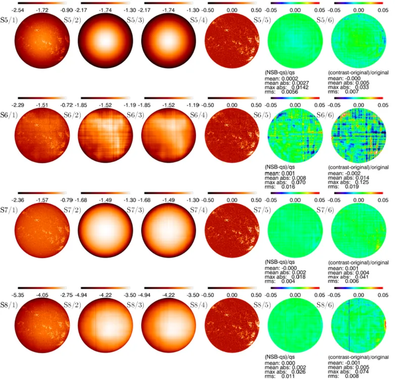
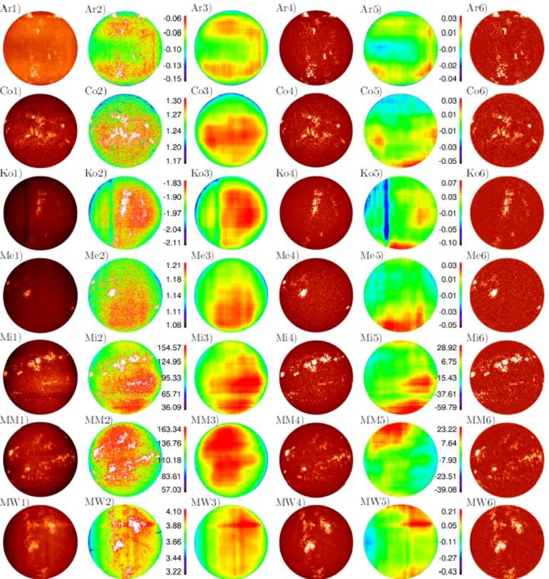
We have applied the proposed method to many SHG ran-domly selected from the seven available historical (photo-graphic) archives. Figures 13 and 14 show examples of the results obtained from observations taken at periods of high and low solar activity, respectively. From left to right, each panel shows the original observation (density image), the density image saturated to show the background, the back-ground (CLV plus inhomogeneities) deduced from the pro-posed processing, the calibrated image, the identified inho-mogeneities of the analysed image, and the final contrast image after the QS CLV removal. From top to bottom each such set of images is shown for SHG extracted from the Ar, Co, Ko, Me, Mi, MM, and MW archives, respectively. All the calibrated images are shown within the intensity range [0.0, 2.0], while the contrast images (i.e. images compen-sated for the CLV) are plotted within [-0.5, 0.5]. For the rest there is a colour bar denoting the range of values. Fur-ther examples can be found in Chatzistergos et al. (2016).
The deduced backgrounds describe the different pat-terns in the analysed images quite accurately. Figures 13 and 14 clearly show that the method works consistently with data extracted from various photographic archives, taken at different activity levels. All calibrated images lie within the same range of values and show a similar CLV pattern. The same is true for the contrast images that re-turn plage regions within the same intensity ranges and no obvious residual large scale artefacts. The method is able to account even for strong inhomogeneities and rather peculiar patterns (e.g. Fig. 13 Ar, or Fig. 14 Ko) without affecting the plage regions. The inhomogeneities identified here show a CLV that is usually off-centred, in many cases having its highest value towards the limb. Furthermore, images show many dark/bright bands that could occur due to something occluding the Sun for a short period, or not constant expo-sure over the different rasters.
The tests on historical observations with good quality, resulted in 1D QS CLV very similar to the one from the Rome/PSPT data. This strengthens our argument that the
Fig. 13. Examples of the calibration procedure of historical images from the Ar, Co, Ko, Me, Mi, MM, MW archives (from top to bottom) taken at high activity periods. From left to right: (1) density images, (2) density images saturated such as to clearly show the backgrounds, (3) calculated backgrounds (CLV and inhomogeneities), (4) calibrated images, (5) identified inhomogeneities, and (6) images corrected for QS CLV. All the unprocessed density images are shown with the whole range of densities within the disc, the calibrated images are shown within the intensity range [0.0, 2.0], while the contrast images (i.e. images compensated for the CLV) are plotted within [-0.5, 0.5]. A colour bar gives the density/intensity range for the rest of the images. The colour bar between images (2) and (3) applies to both images.
CC of the good quality historical data can be described by a linear relation.
Fig. 14. As Fig. 13, but for images taken at low activity periods.
5. Comparison with other methods
5.1. Background calculation methods
We found that the methods presented in the literature that apply radially symmetric computations suffer from their in-ability to account for the asymmetric patterns affecting the images, while application of median filtering suffers under the presence of AR and its inability to account for density variations along adjacent image lines.
By applying the methods of Caccin et al. (1998) and Worden et al. (1998b) on the degraded synthetic SHG we found that these techniques provide inaccurate QS CLV values towards the limb and do not account for small-scale image artefacts, e.g. the density variations in adjacent lines. The method by Tlatov et al. (2009) is also unable to account for these linear artefacts.
Figure 15 shows the pixel by pixel relative differences be-tween the NSB and the imposed background derived with
our method and that by Worden et al. (1998a)3, on two
synthetic images from subset 6. Part of the AR remained undetected by the latter method and so enters the com-putation of the background. Thus the method by Worden et al. (1998a) overestimates the actual background in some plage areas and introduces processing errors in recovering the NSB. The maximum relative errors in NSB are lower for observations taken at low solar activity (3.7%), than at periods of high solar activity (26%), but on average the method by Worden et al. (1998a) introduces one order of magnitude higher errors over the disc than obtained from our proposed method.
We applied the method by Priyal et al. (2013) on all data of subset 6 and we found that the method by Priyal et al. (2013) works reasonably well on images with weak anisotropies, but consistently fails to account for the large inhomogeneities affecting the data, by introducing up to 16 (25) times larger maximum (RMS) errors than those from our method. Besides, the method by Priyal et al. (2013) does not allow recovering any image patterns that occur in a direction different from the one considered for the fit.
5.2. Calibration methods
We tested the accuracy of the method by Priyal et al. (2013) by applying an average CC to calibrate a whole dataset with our synthetic data. We derived the average CC from the curves we imposed to all the data of subset 8, and stud-ied the differences between contrast images obtained from the original data and the ones resulting from the calibration with the average CC. We used the imposed background of each image to compensate for the limb darkening, in order to avoid any other uncertainties of our procedure. This er-ror estimate can be considered only as a lower limit, since the CC used to derive the average were the imposed ones, therefore without taking into consideration any errors in the calculation of the individual CC. Figure 16 shows that the errors introduced by the calibration with the average CC as proposed by the method by Priyal et al. (2013) are on aver-age ∼50%. These errors reach values as high as 300% for a few cases. We stress, however, that we cannot rule out that in actual historical data sets the CC display a smaller varia-tion than in our subset 8. Therefore, the above test mainly shows the greater versatility of the present technique for handling a range of CC values.
Figure 17 shows two examples of Ko images processed with our method (left panels) and by Priyal et al. (2013)4.
The input data employed for this comparison come from different digitizations of the same observation. This limits our analysis of the results to qualitative aspects only. Our images were saturated at the same level to illustrate all AR clearly, however the data by Priyal et al. (2013) were provided in JPG file format and hence we are unable to saturate the images to the same level. Still, Fig. 17 clearly shows that images processed by Priyal et al. (2013) are 3 When we applied the method by Worden et al. (1998a) we
did not perform the last step of the low-pass filtering, because the information of the window-width or the way they applied it on regions very close to the limb is not described. Applying this step could potentially reduce the errors of isolated pixels, but it would not make a difference in the misidentification of the AR.
4
Available at http://kso.iiap.res.in/data
Fig. 15. Relative error in NSB calculation with our method (c– d) and the method by Worden et al. (1998a, e–f) for two images of subset 6 with the lowest level of inhomogeneities (density images shown on a–b). The facular pattern was derived from the Rome/PSPT observations taken on 21/08/2000 (left) and 09/08/2008 (right). Also given (below the images) are the val-ues of the RMS, mean, mean absolute and maximum relative differences within the disc up to 0.98R. The colour bars apply to the images below them.
affected by uncorrected inhomogeneities, to a significantly larger extent than images processed by our method.
In the image processing suggested by Tlatov et al. (2009), all image values are termed intensities and are fur-ther scaled linearly to the values of the standardized profile, without conversion to density values as expected by pho-tographic theory, therefore this method merely applies a linear scaling to the image to let it match a desired range of intensity values. Also the standardised CLV that is taken from Pierce & Slaughter (1977) does not accurately repre-sent the Ca II K data since it corresponds to 390.928 nm. Figure 18 shows the relative difference between results de-rived from the application of the method by Tlatov et al.
Fig. 16. Left: Relative error for the contrast images derived from the calibration with the average CC as suggested by Priyal et al. (2013) of all the synthetic images of subset 8. The maximum differences are divided by 10. Note that the red line (maximum value of the unsigned relative difference) has been divided by 10 to allow it to be plotted together with the other curves. The solid lines are 100 point averages and the shaded surfaces denote the asymmetric 1σ interval. Right: Distribution of the relative difference values.
(2009) and our method to one synthetic image from sub-set 1 produced from the contrast Rome/PSPT observation shown in Fig. 7 S1. The image calibrated with the method of Tlatov et al. (2009) displays a significant offset ∼0.7 and fainter plage and dark regions than in the original image (contrast of ∼0.1 and ∼0.5 obtained by the method of Tla-tov et al. 2009, and ours, respectively).
The method by Ermolli et al. (2009b) cannot be tested on the synthetic data, since it relies on information of the unexposed regions of the plate that we cannot replicate in a meaningful way in the synthetic data.
Finally, we compared the CC computed with our tech-nique and from the calibration wedges stored on Ar data.
Since our method sets the QS near the solar disc cen-tre to be around 1, whereas the wedges describe the re-sponse of the whole plate and contain no information as to which range the QS corresponds, there is a scaling factor between the images calibrated with our method and with the wedges. This factor depends mostly on the digitization (i.e. the range of values of the QS in the digital files), but also on other factors (e.g. slightly different exposure time should change the location of the QS in the CC). Thus, a direct comparison of the CC derived from the two methods is not straightforward.
To account for the difference in values range, we de-rived the CC from the wedges by applying a polynomial fit (Ermolli et al. 2009a), used this CC to calibrate the CLV calculated with our method and then rescaled it to match the range of values in the calibrated CLV derived with our method. Since information is lost with the rescaling, this approach does not allow any conclusion on the slope of the CC. Nonetheless, in this way we can test the assumption of using a linear curve to calibrate these data, provided the fit-ting of the wedge measurements is done accurately enough. However, this may not happen for all Ar data, because of insufficient or inaccurate information stored on the wedges. The wedges of the Ar data usually consist of 3 scans for 7 known exposures, giving 7 points in intensities to fit the sig-moid CC. These values do not necessarily cover the whole range of values on the disc, or even if they do their number may be too low to describe a sigmoid function.
Fig. 17. Examples of calibrated and CLV compensated images from the Ko archive derived with our method (left) and with the method of Priyal et al. (2013, right); the latter data were taken from the Kodaikanal website. The results from Priyal et al. (2013, right) are given in JPG files and shown here unsaturated, while the results from our processing are saturated in the range [-0.5, 0.6]. The observations were taken on 05/08/1947 (top) and 01/01/1964 (bottom).
Figure 19 shows an example of a derived CC for one Ar observation including the rescaled wedge measurements and fit. This is one of the good cases where the CC derived with our method matches almost perfectly the one derived from the wedges, missing only a small part of underexposed regions. It is important to note that the scatter of the values derived from the wedges is almost the same as the scatter in the background of the image. We achieve pixel by pixel relative differences between the image calibrated with our method and that with the wedge that are < 5%, which is consistent with the results presented with the synthetic data from subset 6 (the example tested here was found to have inhomogeneities with a range within 0.6 that of the CLV).
6. Conclusions
We have developed a new method to photometrically cal-ibrate the historical full-disc Ca II K SHG and to correct them for various artefacts of solar and non-solar origin. The method is based on the standardization of the QS CLV intensity pattern to the one resulting from modern obser-vations, under the assumption that it does not vary with time. Modern observations suggest that this holds within the accuracy of the proposed method. We showed that the errors introduced by the above assumptions are relatively small and have minor impact on the CLV estimation un-less the analysed observation is of very poor quality. We assume that QS regions store all the information required to construct the CC for the range of brightnesses covered by the QS anywhere on the solar disc. This is not fulfilled
Fig. 18. Relative error of the calibrated (top) and the con-trast images (bottom) produced after linear calibration with our method (left) and the method of Tlatov et al. (2009, right) for an image of subset 1. The facular pattern was derived from a Rome/PSPT observation taken on 21/08/2000 (shown in Fig. 7 S1). Also listed are the values of the RMS, mean, mean absolute and maximum relative differences by comparing image regions within 0.98R. The colour bars apply to the images below them and are different for each image.
for observations with strong over-exposure effects, as these introduce errors into the bright plage regions near the cen-tre of the solar disc, that cannot be calibrated away by our method. Therefore very poor quality observations must be rejected. However, they constitute a very small fraction of the available historical data. In addition, it can be that only part of the characteristic curve is accurately represented by the QS density values and the assumed linear relation. This would affect mostly plage regions near disc centre or fainter regions towards the limb and can limit the accuracy of our processing. However, we showed that in spite of these poten-tial shortcomings, our method results in much lower errors than different approaches presented in the literature.
To test the accuracy of the proposed method, we cre-ated a large number of synthetic images emulating various problems encountered in historical observations. The max-imum error of our method is < 6.5% averaged over all the degradations studied here, while the average error is < 1%. These errors were derived on synthetic data including ex-treme cases of imposed artefacts. The maximum errors re-duce to < 2% if we exclude images with the most extreme artefacts. Application of other methods for the processing of SHG presented in the literature, returns errors that are between 3 and 300 times larger than those derived from our method.
Fig. 19. Left : Standardized CC derived from our method (red, extrapolated to the range of values of the whole disc), mea-sured CC for the QS (orange) with 1σ uncertainty (black), the whole background (blue), calibration wedge measurements and fit (green rhombuses and line, respectively) of Ar observation taken on 20/07/1948. Shown also is the slope of the derived CC. Right : Distribution of densities for the QS (blue), AR (red) and whole disc (black). The horizontal dashed line in both panels denotes the highest value of the QS CLV.
We also estimated the accuracy of processing modern Ca II K data by applying the proposed method to synthetic images unaffected by linear artefacts. The error estimates decreased by almost a factor of 2 with respect to those reported earlier, with maximum relative errors being on average < 0.6%.
Finally, we applied for test purposes the proposed method to a sample of images randomly extracted from seven historical SHG archives. We showed that the method allows us to process images from different archives consis-tently, without having to adjust or tailor the method to observations taken with different instruments at various ob-servatories and at times of different levels of solar activity. The results of the application of the proposed method to various SHG archives will be presented in a forthcoming paper.
It is worth noting that our method to derive the CLV can be applied with minor adjustments to full-disc solar observations taken in other spectral ranges than Ca II K. Examples are archival white-light photographic images used for identifying and measuring sunspot properties (e.g. Ravindra et al. 2013; Willis et al. 2013; Hanaoka 2013), or SHG in the Hα line (e.g. Mein & Ribes 1990; Pötzi 2008; Garcia et al. 2011; Hanaoka 2013).
Acknowledgements. We thank Dr. Tlatov for providing data pro-cessed with his method and for providing feedback on his method of calibrating SHG. The authors thank the Arcetri, Coimbra, Ko-daikanal, McMath-Hulbert, Meudon, Mitaka, Mt Wilson, and the Rome Solar Groups. T.C. thanks the INAF Osservatorio astronomico di Roma solar physics group for their hospitality during his lengthy visits. T.C. acknowledges postgraduate fellowship of the International Max Planck Research School on Physical Processes in the Solar Sys-tem and Beyond. This work was supported by grants PRIN-INAF-2014 and PRIN/MIUR 2012P2HRCR "Il Sole attivo", COST Ac-tion ES1005 "TOSCA", FP7 SOLID, and by the BK21 plus program through the National Research Foundation (NRF) funded by the Min-istry of Education of Korea.
References
Babcock, H. W. & Babcock, H. D. 1955, The Astrophysical Journal, 121, 349
Ball, W. T., Unruh, Y. C., Krivova, N. A., et al. 2012, Astronomy and Astrophysics, 541, A27
Bertello, L., Ulrich, R. K., & Boyden, J. E. 2010, Solar Physics, 264, 31
Bühler, D., Lagg, A., & Solanki, S. K. 2013, Astronomy and Astro-physics, 555, A33
Brandt, P. N. & Steinegger, M. 1998, Solar Physics, 177, 287 Caccin, B., Ermolli, I., Fofi, M., & Sambuco, A. M. 1998, Solar
Physics, 177, 295
Chapman, G. A., Cookson, A. M., & Preminger, D. G. 2013, Solar Physics, 283, 295
Chatterjee, S., Banerjee, D., & Ravindra, B. 2016, The Astrophysical Journal, 827, 87
Chatzistergos, T., Ermolli, I., Solanki, S. K., & Krivova, N. A. 2016, in Astronomical Society of the Pacific Conference Series, Vol. 504, Coimbra Solar Physics Meeting: Ground-based Solar Observations in the Space Instrumentation Era, ed. I. Dorotovic, C. E. Fischer, & M. Temmer, San Francisco, 227–231
Dainty, J. C. & Shaw, R. 1974, Image science. Principles, analysis and evaluation of photographic-type imaging processes (London: Academic Press)
Dasi-Espuig, M., Jiang, J., Krivova, N. A., & Solanki, S. K. 2014, Astronomy and Astrophysics, 570, A23
Dasi-Espuig, M., Jiang, J., Krivova, N. A., et al. 2016, Astronomy and Astrophysics, 590, A63
Delaygue, G. & Bard, E. 2011, Climate Dynamics, 36, 2201
Denker, C., Johannesson, A., Marquette, W., et al. 1999, Solar Physics, 184, 87
Ermolli, I., Criscuoli, S., Centrone, M., Giorgi, F., & Penza, V. 2007, Astronomy and Astrophysics, 465, 305
Ermolli, I., Criscuoli, S., & Giorgi, F. 2011, Contributions of the As-tronomical Observatory Skalnate Pleso, 41, 73
Ermolli, I., Fofi, M., Bernacchia, C., et al. 1998, Solar Physics, 177, 1 Ermolli, I., Marchei, E., Centrone, M., et al. 2009a, Astronomy and
Astrophysics, 499, 627
Ermolli, I., Matthes, K., Dudok de Wit, T., et al. 2013, Atmospheric Chemistry & Physics, 13, 3945
Ermolli, I., Solanki, S. K., Tlatov, A. G., et al. 2009b, The Astrophys-ical Journal, 698, 1000
Fredga, K. 1971, Solar Physics, 21, 60
Fröhlich, C. 2013, Space Science Reviews, 176, 237
Garcia, A., Sobotka, M., Klvana, M., & Bumba, V. 2011, Contribu-tions of the Astronomical Observatory Skalnate Pleso, 41, 69 Gardner, I. C. 1947, Validity of the cosine-fourth-power law of
illumi-nation (National Bureau of Standards)
Giorgi, F., Ermolli, I., Centrone, M., & Marchei, E. 2005, Memorie della Societa Astronomica Italiana, 76, 977
Goldman, D. & Chen, J.-H. 2005, in Tenth IEEE International Con-ference on Computer Vision, 2005. ICCV 2005, Vol. 1, 899–906 Vol. 1
Haigh, J. D. 2007, Living Reviews in Solar Physics, 4, 2
Hanaoka, Y. 2013, Journal of Physics Conference Series, 440, 2041 Harvey, K. L. & White, O. R. 1999, The Astrophysical Journal, 515,
812
Johannesson, A., Marquette, W. H., & Zirin, H. 1998, Solar Physics, 177, 265
Kahil, F., Riethmüller, T. L., & Solanki, S. K. 2017, The Astrophysical Journal Supplement Series, 229, 12
Kariyappa, R. & Pap, J. M. 1996, Solar Physics, 167, 115 Kariyappa, R. & Sivaraman, K. R. 1994, Solar Physics, 152, 139 Kopp, G. 2016, Journal of Space Weather and Space Climate, 6, A30 Krivova, N. A., Balmaceda, L., & Solanki, S. K. 2007, Astronomy and
Astrophysics, 467, 335
Krivova, N. A., Solanki, S. K., Fligge, M., & Unruh, Y. C. 2003, Astronomy and Astrophysics, 399, L1
Krivova, N. A., Vieira, L. E. A., & Solanki, S. K. 2010, Journal of Geophysical Research (Space Physics), 115, 12112
Lean, J., Beer, J., & Bradley, R. 1995, Geophysical Research Letters, 22, 3195
Lefebvre, S., Ulrich, R. K., Webster, L. S., et al. 2005, Memorie della Societa Astronomica Italiana, 76, 862
Lites, B. W., Centeno, R., & McIntosh, S. W. 2014, Publications of the Astronomical Society of Japan, 66, S4
Livingston, W. & Sheeley, Jr., N. R. 2008, The Astrophysical Journal, 672, 1228
Livingston, W. & Wallace, L. 2003, Solar Physics, 212, 227
Livingston, W., Wallace, L., White, O. R., & Giampapa, M. S. 2007, The Astrophysical Journal, 657, 1137
Loukitcheva, M., Solanki, S. K., & White, S. M. 2009, Astronomy and Astrophysics, 497, 273
Makarov, V. I., Tlatov, A. G., & Callebaut, D. K. 2004, Proceedings of the International Astronomical Union, 2004, 49
Mein, P. & Ribes, E. 1990, Astronomy and Astrophysics, 227, 577 Mickaelian, A. M., Nesci, R., Rossi, C., et al. 2007, Astronomy and
Astrophysics, 464, 1177
Nesme-Ribes, E., Meunier, N., & Collin, B. 1996, Astronomy and Astrophysics, 308, 213
Peck, C. L. & Rast, M. P. 2015, The Astrophysical Journal, 808, 192 Pierce, A. K. & Slaughter, C. D. 1977, Solar Physics, 51, 25 Priyal, M., Singh, J., Ravindra, B., Priya, T. G., & Amareswari, K.
2013, Solar Physics
Pötzi, W. 2008, Central European Astrophysical Bulletin, 32, 9 Ravindra, B., Priya, T. G., Amareswari, K., et al. 2013, Astronomy
and Astrophysics, 550, 19
Schrijver, C. J., Cote, J., Zwaan, C., & Saar, S. H. 1989, The Astro-physical Journal, 337, 964
Shapiro, A. I., Schmutz, W., Rozanov, E., et al. 2011, Astronomy and Astrophysics, 529, 67
Singh, J., Belur, R., Raju, S., et al. 2012, Research in Astronomy and Astrophysics, 12, 472
Skumanich, A., Smythe, C., & Frazier, E. N. 1975, The Astrophysical Journal, 200, 747
Solanki, S. K. & Fligge, M. 2000, Space Science Reviews, 94, 127 Solanki, S. K., Krivova, N. A., & Haigh, J. D. 2013, Annual Review
of Astronomy and Astrophysics, 51, 311
Steinhilber, F., Beer, J., & Fröhlich, C. 2009, Geophysical Research Letters, 36, L19704
Tlatov, A. G., Pevtsov, A. A., & Singh, J. 2009, Solar Physics, 255, 239
Vieira, L. E. A., Solanki, S. K., Krivova, N. A., & Usoskin, I. 2011, Astronomy and Astrophysics, 531, 6
Walton, S. R., Chapman, G. A., Cookson, A. M., Dobias, J. J., & Preminger, D. G. 1998, Solar Physics, 179, 31
Wang, Y.-M., Lean, J. L., & Sheeley, Jr., N. R. 2005, The Astrophys-ical Journal, 625, 522
White, O. R. & Livingston, W. 1978, The Astrophysical Journal, 226, 679
White, O. R. & Livingston, W. C. 1981, The Astrophysical Journal, 249, 798
Willis, D. M., Coffey, H. E., Henwood, R., et al. 2013, Solar Physics, 288, 117
Worden, J. R., White, O. R., & Woods, T. N. 1998a, The Astrophys-ical Journal, 496, 998
Worden, J. R., White, O. R., & Woods, T. N. 1998b, Solar Physics, 177, 255
Yeo, K. L., Krivova, N. A., Solanki, S. K., & Glassmeier, K. H. 2014, Astronomy and Astrophysics, 570, A85
Zharkova, V. V., Ipson, S. S., Zharkov, S. I., et al. 2003, Solar Physics, 214, 89