DOTTORATO DI RICERCA IN
Ingegneria Elettrotecnica
Ciclo XXVIII
Settore Concorsuale di afferenza: 09/E2 Settore Scientifico disciplinare: ING-IND/33
INSULATION COORDINATION
IN MODERN DISTRIBUTION NETWORKS
Presentata da: Ing. Fabio Tossani
Coordinatore Dottorato
Relatore
Prof. Domenico Casadei
Prof. Carlo Alberto Nucci
Introduction ... 3
1. Lightning Induced Overvoltages on Multiconductor Lines ... 5
1.1. Lightning Electromagnetic Pulse Appraisal ... 5
1.2. Lightning Electromagnetic Pulse Coupling to Multi-Conductor Lines ... 9
1.2.1. The Agrawal, Price and Gurbaxani model ... 9
1.2.2. The LIOV Code ... 10
1.2.3. Fields and Overvoltages due to a Stroke Location Close to the Line ... 12
1.3. Transient Ground Resistance of Multiconductor Lines ... 19
1.3.1. Inverse Laplace Transform of Sunde’s Logarithmic Formula – The Series Expression ... 19
1.3.2. Inverse Laplace Transform of Sunde’s Logarithmic Formula – The Integral Expression ... 32
1.3.3. Inverse Laplace Transform of Sunde’s Integrals ... 38
1.4. The Response of Multi-Conductor Lines to Lightning-Originated Electromagnetic Pulse ... 43
2. Statistical Evaluation of the Lightning Performance of Distribution Networks ... 58
2.1. The Lightning Performance of Overhead Distribution Lines ... 58
2.2. The Influence of Direct Strikes on the Lightning Performance of Overhead Distribution Lines ... 63
2.3. The Effect of the Channel Base Current Waveform on the Lightning Performance of Overhead Distribution Lines ... 73
2.4. Lightning Performance of a Real Distribution Network with Focus on Transformer Protection ... 89
3. Conclusion ... 106
4. Appendix 1 – Inverse Laplace transform of Ground Impedance Matrix – case 1: Sunde’s Logarithmic formula ... 108
5. Appendix 2 – Inverse Laplace transform of Ground Impedance Matrix – case 2: Sunde’s Integral formula... 110
Introduction
Lightning is a major cause of faults on typical overhead distribution lines. These faults may cause momentary or permanent interruptions on distribution circuits. Power-quality concerns have created more interest in lightning, and as a consequence improved lightning protection of overhead distribution lines against faults is being considered as a way to reduce the number of momentary interruptions and voltage sags (IEEE Std 1410-2010, 2011).
For the above reasons, the problem of lightning protection of overhead and buried power lines has been reconsidered in recent years due to the proliferation of sensitive loads and the increasing demand by customers for good quality in the power supply (Nucci et al., 2012). This leads to specific requirements concerning insulation and protection coordination, which need also to take into account the presence of distributed generation and of the evolving topology/structure of the smart grid.
Another aspect that deserves proper attention is that in modern distribution networks there is an increasing number of distribution system operators interested in changing the earthing method from solidly grounded to resonant one. This makes it crucial to distinguish single-phase to ground faults from other types of faults. In addition to that, the increasing development and wider interconnection of smart grids leads to more complex network structure and dynamic behaviors.
The appropriate analysis of the response of distribution networks against Lightning Electro Magnetic Pulse (LEMP) requires therefore the availability of more accurate models of LEMP-illuminated lines with respect to the past in order to reproduce the real and complex configuration of distribution systems including the presence of shield wires and of their groundings, as well as that of surge arresters and distribution transformers.
From the distribution system operator point of view, the above models represent a fundamental tool for achieving the estimate of the number of protective devices and of their most appropriate location in order to guarantee a given minimum number of flashovers and outages per year. When dealing with real networks, such an optimization could require huge computational efforts due to the vast number of power components and feeders present in real power systems. This thesis thoroughly analyzes many of the possible engineering
simplifications that, without losing accuracy, can be adopted in the statistical evaluation of the lightning performance of distribution networks in order to limit computational times.
The structure of this thesis is the following:
Chapter one begins with a brief description of the expression adopted in this thesis for the
evaluation of the lightning electromagnetic pulse (LEMP). The calculation of the induced voltages is performed by using the LIOV code (Lightning induced overvoltages) which is based on the coupling model by Agrawal et al (1980). Particular attention is devoted to the effect of the ground conductivity on the LEMP and on the line parameters. In this regard, this thesis proposes two new analytical expressions for the evaluation of the inverse Laplace transform of the ground impedance matrix elements of a multiconductor overhead line. The first expression is the inverse Laplace transform of Sunde’s logarithmic formula (Sunde, 1968) and is given in two equivalent forms. The second expression is the inverse Laplace transform of the general integral expression given by Sunde (1968). The mathematical derivation of the latter is then extended to the classical case of a multiconductor buried line (Pollaczek, 1926) taking into account also the displacement currents (Sunde, 1968).
Chapter two is devoted to the statistical evaluation of the lightning performance of
distribution networks. The analysis begins with the case of a straight line and discusses the effect of the lightning base channel waveform and of the taking into account of direct strikes on the lightning performance. Finally, a procedure able to evaluate the lightning performance of a real medium-voltage distribution network, which includes a number of lines, transformer stations and surge protection devices is developed and proposed for the analysis of some real cases. Such a procedure allows inferring the characteristics of the statistical distributions of lightning-originated voltages at any point and at any phase of the network. The analysis aims at assessing the expected mean time between failures of MV/LV transformers caused by both direct and indirect lightning strikes. A heuristic technique has been specifically developed to reduce the computational effort despite the non-linear response of the network equipped with surge arresters.
1. Lightning Induced Overvoltages on
Multiconductor Lines
1.1. Lightning Electromagnetic Pulse Appraisal
The expressions in time domain of the electromagnetic field radiated by a vertical dipole of length dz’ at a height z' along the lightning channel, assumed as an antenna over a perfectly conducting plane, have been derived by Master & Uman (1983) by solving Maxwell's equations in terms of retarded scalar and vector potentials:
(
)
(
)
(
)
(
)
(
)
(
) (
)
(
)
(
)
(
)
5 0 0 4 2 3 2 2 5 0 0 3 ' ' , , ', / 4 3 ' ', / ' ', / 2 ' ' , , ', / 4 t r t z r z z dz dE r z t i z R c d R r z z i z t R c cR r z z i z t R c t c R z z r dz dE r z t i z R c d R t t πε t t πε é -ê = ê - + ë -+ - + ù - ¶ - ú + ú ¶ û é - -ê = ê - + êë +ò
ò
(
)
(
)
(
)
(
)
(
)
(
)
2 2 4 2 2 3 0 3 2 2 ' ', / ', / ' , , ', / 4 ', / + z z r i z t R c cR i z t R c r t c R dz r dB r z t i z t R c R i z t R c r t cR ϕ µ π - -- + ù ¶ - ú - ú ¶ û é ê = -êë ù ¶ - ú ú ¶ û (1.1) where− i(z', t) is the current along the channel obtained from the return-stroke current model; − c is the speed of light;
− R is the distance of the electric dipole from the observation point; and the geometrical factors are given in Figure 1-1.
z' H IMMAGINE dz' i(z',t) R R' r x y ZL z z' P (x,y,z) Z o E h E r z E E Ex P(x,y,z) φ
v
Figure 1-1 – Return Stroke channel
By integrating expressions (1.1) along the channel one obtains the electromagnetic exciting field. The current distribution, as a function of height and time, is given by the so called return-stroke model (Nucci et al., 1990), (Rakov & Uman, 1998).
For distances not exceeding a few kilometers, the perfect ground conductivity assumption is a reasonable approximation for the vertical component of the electric field and for the azimuthal component of the magnetic field (Zeddam & Degauque, 1990). This can be explained considering that the contributions of the source dipole and of its image to these field components add constructively and, consequently, small variations in the image field due to the finite ground conductivity will have little effect on the total field. On the other hand, the horizontal component of the electric field is appreciably affected by finite ground conductivity. Indeed, for such a field component, the effects of the two contributions subtract, and small changes in the image field may lead to appreciable changes in the total horizontal field (Rubinstein, 1996). Although the intensity of the horizontal field component is generally much smaller than that of the vertical one, within the context of certain coupling models it plays an important role in the coupling mechanism (Master & Uman, 1984; Cooray & De la
Rosa, 1986; Rubinstein et al., 1989; Diendorfer, 1990; Ishii et al., 1994) and, hence, an accurate
The exact solution for the problem of an oscillating hertzian dipole over a finite ground is due to Sommerfeld (1909) and in terms of magnetic vector potential is given by (Sommerfeld, 1949)
(
)
(
)
( )
' 0 ( ' ) 0 2 0 ', ' 2 , , 4 ' j R j R c c z z E z E I z j dz e e dA j r z J r e d R R n ω ω µ µ ω µ λ ω λ λ π µ µ µ ¥ - + æ ö÷ ç ÷ ç ÷ ç ÷ = çç + - ÷ ÷ + ç ÷÷ çèò
ø (1.2) where, 2 2 0 0 k =ω µ ε
2 2 0 E r k =ω ε ε µ ω µσ
+ j 2 2 2 / E n =k k and 2 2 k µ= λ - (1.3) 2 2 E kE µ = λ - (1.4)where I j
( )
ω is the current of the dipole in the frequency domain, ω is the angular frequency,J0 is the Bessel function of the first kind of order zero, and j2 = –1. The first two terms in (1.2)
are the components of the magnetic vector potential in case of perfect ground; the latter is the Sommerfeld integral, which is present only in case of lossy ground.
The non-null components of the electromagnetic field in the frequency domain due to the dipole can be obtained from the magnetic vector potential by
(
)
(
)
(
)
2 2 2 2 2 2 0 1 z r z z z z A j E j r z r z k A j E j r z k A k z A H j r z r ϕ ω ω ω ω ω µ ¶ , , = ¶ ¶ æ¶ ö÷ ç ÷ , , = çç + ÷÷ ç ¶ è ø ¶ , , = -¶ . (1.5)Performing this operation one obtains the electromagnetic field in frequency domain for z > 0. The fields in case of ideal ground can be directly transformed in time domain and are given by (1.1). In case of lossy ground, the following contributions should be added to (1.1):
(
)
( )
( )
(
)
( )
( )
(
)
( )
( )
( ' ) 2 1 2 0 0 3 ( ' ) 0 2 0 0 2 ( ' ) 1 2 0 ' 2 ' 2 ' 2 z z E r E z z E z E z z E E I j dz dE j r z j J r e d n I j dz dE j r z j J r e d n I j dz dH j r z J r e d n µ µ µ ϕ ω µ ω λ λ λ πωε µ µ ω µ λ ω λ λ πωε µ µ µ ω µ λ ω λ λ π µ µ µ ¥ - + ¥ - + ¥ - + , , = -+ , , = -+ , , = -+ò
ò
ò
(1.6)The total electric and magnetic field is obtained by summing the time-domain contribution of each dipole, taking into account the time delays associated with finite speed of propagation of return stroke front and the electromagnetic fields in air. Recently (F. Delfino, Procopio, and
Rossi 2008; F. Delfino et al. 2008) numerical techniques that can be utilized to perform these
integrals rapidly and efficiently have been developed. However, when the evaluation of the LEMP for a large number of observation points is needed (e.g. when assessing the induced voltages in a real network or in statistical procedures) the calculation of the horizontal field using the exact Sommerfeld integrals is inefficient from the point of view of computer-time. Many simplified expressions exist, and the most commonly adopted one is that proposed independently by Cooray and Rubinstein (Cooray, 1992; Rubinstein, 1996) and discussed by
Wait (1997). The Cooray-Rubinstein expression is given by
(
, ,)
(
, ,)
(
, 0,)
o r rp p E r z jω E r z jω cBφ r z jω γ γ = - = × (1.7) where − γo=ω µ ε0 0 − 0 0 o r jσ γ γ ε ε ε ω =-− σis the ground conductivity;
− Erp(r z j, , ω) e Bφp(r z, =0, jω) are the radial component of the electric field and the
azimuthal component of the magnetic field evaluated as the ground was a perfect conductor
and c is the speed of light in vacuum.
The second term in (1.7) is known in the literature as ‘surface impedance’ expression. The surface impedance expression is in good agreement with the Sommerfeld integrals solution for distances not closer than 50 m from the stroke location for σ = 0.01 S/m, 200 m for σ =
0.001 S/m (100 m if only the peak is concerned) and approximately 600 m for 0.0001 S/m. The error can be significant if this expression is adopted for smaller distances (Cooray, 2010).
1.2. Lightning Electromagnetic Pulse Coupling to
Multi-Conductor Lines
The approach adopted in this thesis stands on the transmission line theory . The basic assumptions of this approximation are that the response of the line is quasi-transverse electromagnetic (quasi-TEM) and that the transverse dimension of the line is smaller than the minimum significant wavelength. The line is represented by a series of elementary sections which is illuminated progressively by the incident electromagnetic field so that longitudinal propagation effects are taken into account. Different and equivalent coupling models based on the use of the transmission-line approach have been proposed in the literature (e.g., see C. D.
Taylor et al. 1965; Agrawal et al. 1980; Rachidi 1993). The Agrawal model presents the
notable advantage of taking into account in a straightforward way the ground resistivity in the coupling mechanism and it is the only one that has been thoroughly tested and validated using experimental results (Nucci & Rachidi, 2003),(Paolone et al., 2009).
1.2.1. The Agrawal, Price and Gurbaxani model
The coupling equations according to the Agrawal et al. model are given by (Agrawal et al., 1980)
( )
, '[
( , )]
(
, ,)
s e i ij i x i v x t L i x t E x h t x t ¶ é ù é ù ¶ é ù +ê ú = ê ú ë û ê ú ë û ë û ¶ ¶ (1.8)( )
, ' s( , ) 0 i ij i i x t C v x t x t ¶ é ù +é ù ¶ é ù = ê ú ê ú ë û ë û ë û ¶ ¶ (1.9) where− éêëExe
(
x h t, ,i)
ùúû is the vector of the horizontal component of the incident electric field (calculated in absence of the line conductors) along the x axis at the conductor’s height− [ ' ]Lij and [ ' ]C ij are the matrices of the line per-unit-length inductances and capacitances respectively;
− [ ( , )]i x ti is the line current vector;
− [ ( , )]v x tis is the scattered voltage vector, from which the total voltage vector[v x ti( , )]can
be evaluated as where
(
)
0 ( , ) ( , ) , , i h s e i i z v x t v x t E x z t dz é ù ê ú é ù é= ù- ê ú ê ú ê ú ë û ë û ê ú ëò
û (1.10)− Eze
(
x z t, ,)
is the vertical component of the incident electric field (calculated in absence of the line conductors).Let us assume that the line is terminated on linear terminations represented by the matrices 0,
[Z ij] and [ZL ij, ]. The boundary conditions are given by
( )
(
)
0, 0 (0, ) 0, 0, , i h s e i ij i z v t Z i t E z t dz é ù ê ú é ù= -éê ù éú ù+ ê ú ê ú ë ûë û ë û ê ú ëò
û (1.11)( )
(
)
, 0 ( , ) , , , i h s e i L ij i z v L t Z i L t E L z t dz é ù ê ú é ù é=ê ù éú ù+ ê ú ê ú ë ûë û ë û ê ú ëò
û (1.12)1.2.2. The LIOV Code
In the literature, several approaches have been proposed for the evaluation of the lightning electromagnetic pulse (LEMP) response of distribution networks (e.g., Nucci et al. (1994),
Orzan et al. (1996), Høidalen (2003), Perez et al. (2007), Andreotti et al. (2015), Thang et al.
(2015), and references therein).
In this thesis the LIOV–EMTP-RV code is adopted for the calculation of the induced voltages. LIOV (“Lightning-induced overvoltages”) (Nucci & Rachidi, 2003), (Borghetti et al., 2004), (Napolitano et al., 2008) is a computer code which allows for the calculation of lightning-induced overvoltages on multiconductor overhead lines above a lossy soil as a function of line
geometry, lightning current wave shape and stroke location, return-stroke velocity and soil resistivity.
LIOV has been developed in the framework of an international collaboration involving the University of Bologna, the Swiss Federal Institute of Technology and the University of Rome La Sapienza. LIOV has been experimentally validated by means of tests carried out on reduced scale setups with NEMP (Nuclear Electromagnetic Pulse) simulators (Borghetti et al., 2004), LEMP (Lightning Electromagnetic Pulse) simulators (Piantini et al., 2007) and full scale setups illuminated by artificially initiated lightning (Paolone et al., 2009) .
In order to analyze the response of realistic configurations such as an electrical medium and low-voltage distribution network to a LEMP excitation, the presence of specific line terminations or line discontinuities (e.g. surge arresters) is to be properly taken into account. To deal with the problem of lightning-induced voltages on complex systems, different interfacing methods between LIOV and EMTP were developed (Nucci et al., 1994), (Borghetti
et al., 2004), (Napolitano et al., 2008).
For the LEMP-to-line coupling solution, LIOV adopts the Agrawal et al. model, under the assumption that the response of the line is TEM (or quasi-TEM if the effect of the line losses is accounted in the surge propagation). The Agrawal et al. transmission line equations are solved by means of a one-dimensional Finite Difference Time Domain (FDTD) technique (Nucci et al., 1994), (Borghetti et al., 2004), (Napolitano et al., 2008). In particular, a second order FDTD scheme is adopted, according to which the line length is discretized in a finite number of nodes, at which scattered voltages, currents and the horizontal component of the external electromagnetic field are evaluated at each time step (Paolone et al., 2001), (Nucci &
1.2.3. Fields and Overvoltages due to a Stroke Location Close to the Line
The presence of objects nearby distribution lines may cause indirect overvoltages due to very close lightning return strokes. In these cases, the evaluation of the LEMP by using the Cooray-Rubinstein approach may lead to significant errors. Furthermore, when calculating the incident voltage, the numerical evaluation of integral (1.10) is necessary, due to the height-dependence of the integrand. In the following, the analysis of fields and overvoltages due to a return stroke close to a distribution line is presented.
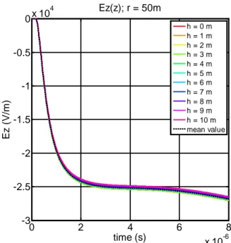
Figure 1-2 and Figure 1-4 show the vertical component of the electric field at a distance r = 10 m from the lightning channel for a typical first stroke and subsequent stroke respectively. The comparison is performed at different heights above an ideal ground, showing that the vertical component of the electric field is strongly dependent on the height z (h in the figures). The mean value is also reported. In Figure 1-3 and Figure 1-5 the same comparison is shown but at a distance r = 20 m from the lightning channel and in Figure 1-6 and Figure 1-7 at a distance r = 50 m; it is clear that, as r increases, the vertical component tends to be constant with height. One can conclude that, if the stroke position is close to a line, the vertical component of the electric field has to be integrated along the coordinate z in (1.10). When the stroke distance is greater or equal 50 m, considering the vertical electric field constant with height is a good approximation.
TABLE 1-1– PARAMETERS ASSUMED FOR THE RETURN STROKE CURRENTS
Figure 1-2 – Vertical component of the electric field for r = 10 m, at different heights above ideal ground. Channel base current typical of first strokes.
Figure 1-3 – Vertical component of the electric field for r = 20 m, at different heights above ideal ground. Channel base current typical of first strokes.
Figure 1-4 – Vertical component of the electric field for r = 10 m, at different heights above ideal ground. Channel base current typical of subsequent strokes.
Figure 1-5 – Vertical component of the electric field for r = 20 m, at different heights above ideal ground. Channel base current typical of subsequent strokes.
0 0.5 1 1.5 x 10⁻⁵ -7 -6 -5 -4 -3 -2 -1 0x 10 5 Ez ( V/ m ) time (s) Ez(z); r = 10m h = 0 m h = 1 m h = 2 m h = 3 m h = 4 m h = 5 m h = 6 m h = 7 m h = 8 m h = 9 m h = 10 m mean value 0 0.5 1 1.5 x 10⁻⁵ -3.5 -3 -2.5 -2 -1.5 -1 -0.5 0x 10 5 Ez ( V/ m ) time (s) Ez(z); r = 20m h = 0 m h = 1 m h = 2 m h = 3 m h = 4 m h = 5 m h = 6 m h = 7 m h = 8 m h = 9 m h = 10 m mean value 0 2 4 6 8 x 10⁻⁶ -15 -10 -5 0x 10 4 Ez ( V/ m ) time (s) Ez(z); r = 10m h = 0 m h = 1 m h = 2 m h = 3 m h = 4 m h = 5 m h = 6 m h = 7 m h = 8 m h = 9 m h = 10 m mean value 0 2 4 6 8 x 10⁻⁶ -8 -7 -6 -5 -4 -3 -2 -1 0x 10 4 Ez ( V/ m ) time (s) Ez(z); r = 20m h = 0 m h = 1 m h = 2 m h = 3 m h = 4 m h = 5 m h = 6 m h = 7 m h = 8 m h = 9 m h = 10 m mean value I01 (kA) τ11 (μs) τ12 (μs) n1 I02 (kA) τ21 (μs) τ22 (μs) n2 First stroke 28 1.8 95 2 - - - - Subsequent stroke 10.7 0.25 2.5 2 6.5 2 230 2
Figure 1-6 – Vertical component of the electric field for r = 50 m, at different heights above ideal ground. Channel base current typical of first strokes.
Figure 1-7 – Vertical component of the electric field r = 50 m, at different heights above ideal ground. Channel base current typical of subsequent strokes.
The accurate evaluation of the horizontal component of the electric field in the vicinity of the lightning channel can be performed by using Sommerfeld integrals or a FEM model such as the one described in (Borghetti et al., 2013), which is in very good agreement with the solution of Sommerfeld integrals. A time-domain formula for the calculation of the horizontal electric field in the vicinity of the lightning channel has been present in (Barbosa & Paulino, 2010).
In Figure 1-8, the radial component of the electric field for r = 10 m, at z = 10 m above a lossy ground (σg = 1 mS/m, εr = 10) due to a first stroke current is shown; the black line refers to the
FEM solution, which can be assumed as benchmark, the red one is calculated by using the Cooray-Rubinstein (CR) formula and the blue one by Barbosa et. al formula. The comparison is also reported in Figure 1-10 for the case of a subsequent stroke. The comparison is then repeated for r = 20 m and r = 50 m. As already mentioned, the CR formula can lead to significant errors if used for the evaluation of the horizontal field in the vicinity of the lightning channel (distance lower than 50 m). The formula by Barbosa and colleagues is, instead, in better agreement with the benchmark solution.
0 0.5 1 1.5 x 10⁻⁵ -14 -12 -10 -8 -6 -4 -2 0x 10 4 Ez ( V/ m ) time (s) Ez(z); r = 50m h = 0 m h = 1 m h = 2 m h = 3 m h = 4 m h = 5 m h = 6 m h = 7 m h = 8 m h = 9 m h = 10 m mean value 0 2 4 6 8 x 10⁻⁶ -3 -2.5 -2 -1.5 -1 -0.5 0x 10 4 Ez ( V/ m ) time (s) Ez(z); r = 50m h = 0 m h = 1 m h = 2 m h = 3 m h = 4 m h = 5 m h = 6 m h = 7 m h = 8 m h = 9 m h = 10 m mean value
Figure 1-8 – Radial component of the electric field for r = 10 m, at z = 10 m above a lossy ground (σg = 1
mS/m, εr = 10). Channel base current typical of first
strokes.
Figure 1-9 – Radial component of the electric field for r = 20 m, at z = 10 m above a lossy ground (σg = 1
mS/m, εr = 10). Channel base current typical of first
strokes.
Figure 1-10 – Radial component of the electric field for r = 10 m, at z = 10 m above a lossy ground (σg = 1
mS/m, εr = 10). Channel base current typical of
subsequent strokes.
Figure 1-11 – Radial component of the electric field for r = 20 m, at z = 10 m above a lossy ground (σg = 1
mS/m, εr = 10). Channel base current typical of
subsequent strokes. 0 0.5 1 1.5 x 10⁻⁵ -1 0 1 2 3 4 5x 10 5 E r (V /m) time (s) Er; r = 10 m FEM Cooray Rubinstein Barbosa 0 0.5 1 1.5 x 10⁻⁵ -2 0 2 4 6 8 10 12 14 16x 10 4 E r (V /m) time (s) Er; r = 20 m FEM Cooray Rubinstein Barbosa 0 2 4 6 8 x 10⁻⁶ -2 0 2 4 6 8 10 12x 10 4 E r (V /m) time (s) Er; r = 10 m FEM Cooray Rubinstein Barbosa 0 2 4 6 8 x 10⁻⁶ -0.5 0 0.5 1 1.5 2 2.5 3 3.5x 10 4 E r (V /m) time (s) Er; r = 20 m FEM Cooray Rubinstein Barbosa
Figure 1-12 – Radial component of the electric field for r = 50 m, at z = 10 m above a lossy ground (σg = 1
mS/m, εr = 10). Channel base current typical of first
strokes.
Figure 1-13 – Radial component of the electric field for r = 50 m, at z = 10 m above a lossy ground (σg = 1
mS/m, εr = 10). Channel base current typical of
subsequent strokes.
Let us now consider the geometry reported in Figure 1-14, namely a 1-km long, 10-m high single conductor line with matched terminations.
In Figure 1-15, the comparison between the overvoltages at the mid-point of the line calculated different approaches discussed in this section is reported. The stroke distance from the line is d = 10 m and the ground is characterized by σg = 1 mS/m and εr = 10. The
comparison is performed again for the two different return stroke current considered and for the three distances between the line and the stroke location (namely 10, 20 and 50 m). The overvoltages calculations are performed by using the LIOV code with the different fields provided as input. Considerations similar to the ones done for the horizontal electric field apply. As expected, the importance of integrating the vertical field along the z coordinate is noticeable when the distance from the line is lower than 50 m.
0 0.5 1 1.5 x 10⁻⁵ -0.5 0 0.5 1 1.5 2 2.5 3x 10 4 E r (V /m) time (s) Er; r = 50 m FEM Cooray Rubinstein Barbosa 0 2 4 6 8 x 10⁻⁶ -1000 0 1000 2000 3000 4000 5000 6000 E r (V /m) time (s) Er; r = 50 m FEM Cooray Rubinstein Barbosa
Figure 1-14 – Considered geometry
Figure 1-15 – Overvoltage at point in front of the stroke location. Stroke distance from the line: d = 10 m. Lossy ground with σg = 1 mS/m and εr = 10.
Channel base current typical of first strokes.
Figure 1-16 – Overvoltage at point in front of the stroke location. Stroke distance from the line: d = 20 m. Lossy ground with σg = 1 mS/m and εr = 10.
Channel base current typical of first strokes.
Figure 1-17 – Overvoltage at point in front of the stroke location. Stroke distance from the line: d = 10 m. Lossy ground with σg = 1 mS/m and εr = 10.
Channel base current typical of subs. strokes.
Figure 1-18 – Overvoltage at point in front of the stroke location. Stroke distance from the line: d = 20 m. Lossy ground with σg = 1 mS/m and εr = 10.
Channel base current typical of subsequent strokes.
0 2 4 6 8 x 10⁻⁶ 0 1 2 3 4 5 6 7 8x 10 5 time (s) V o lt age ( V ) CR, h⋅Ez(z=0) CR, ∫ Ez FEM Barbosa, ∫ Ez 0 2 4 6 8 x 10⁻⁶ 0 0.5 1 1.5 2 2.5 3 3.5 4x 10 5 time (s) V o lt age ( V ) CR, h⋅Ez(z=0) CR, ∫ Ez FEM Barbosa, ∫ Ez 0 0.5 1 1.5 2 x 10⁻⁶ 0 1 2 3 4 5 6x 10 5 time (s) V o lt age ( V ) CR, h⋅Ez(z=0) CR, ∫ Ez FEM Barbosa, ∫ Ez 0 2 4 6 8 x 10⁻⁶ 0 0.5 1 1.5 2 2.5 3x 10 5 time (s) V o lt age ( V ) CR, h⋅Ez(z=0) CR, ∫ Ez FEM Barbosa, ∫ Ez
Figure 1-19 – Overvoltage at point in front of the stroke location. Stroke distance from the line: d = 50 m. Lossy ground with σg = 1 mS/m and εr = 10.
Channel base current typical of first strokes.
Figure 1-20 – Overvoltage at point in front of the stroke location. Stroke distance from the line: d = 50 m. Lossy ground with σg = 1 mS/m and εr = 10.
Channel base current typical of subsequent strokes.
0 2 4 6 8 x 10⁻⁶ 0 0.5 1 1.5 2 2.5x 10 5 time (s) V o lt age ( V ) CR, h⋅Ez(z=0) CR, ∫ Ez FEM Barbosa, ∫ Ez 0 2 4 6 8 x 10⁻⁶ -2 0 2 4 6 8 10 12 14 16x 10 4 time (s) V o lt age ( V ) CR, h⋅Ez(z=0) CR, ∫ Ez FEM Barbosa, ∫ Ez
1.3. Transient Ground Resistance of Multiconductor Lines
The effect of losses on the surge propagation along a multiconductor line illuminated by an external electromagnetic field has been treated in quite a few papers by representing the ground losses as an additional longitudinal term in the coupling equations e.g., (Rachidi et al., 1996, 1999, 2003): the so-called ground impedance in the frequency domain, or its time-domain counter-part, the transient ground resistance. Several expressions for the terms of the ground impedance matrix have been proposed e.g., (Sunde, 1968; Carson, 1926; Pollaczek, 1931; Vance, 1978; Gary, 1976) and, within the limits of the transmission line approximation (TL), the most accurate one is considered the one derived by Sunde (1968). Indeed, it can be shown that the general, more rigorous, expressions derived using scattering theory reduce to the Sunde approximation under the transmission line theory assumption (Tesche et al., 1997). So far, analytical expressions for the inverse Fourier transform of the Sunde formula are not available in the literature, thus, the elements of the ground transient resistance matrix in time domain have to be, in general, evaluated adopting a numerical inverse Fourier transform algorithm. A low-frequency approximation for the ground impedance is the well-known expression derived by Carson (1926) and its analytical inverse Fourier transform has been first derived by Timotin (1967) for the case of a single conductor line, and then extended to a multiconductor line by Orzan (1997). The expressions of Timotin and Orzan feature a singularity at t = 0 for the transient ground resistance matrix elements. Rachidi et al. (2003) showed that the singularity is due to the low frequency approximation of the Carson formula. Such singularity is indeed absent in the case of the Sunde formula, according to which the ground transient resistance tends to an asymptotic value when t tends to zero. Combining the asymptotic behavior of the transient ground resistance at early times and the Timotin/Orzan expressions for the late times, Rachidi et al. (2003) proposed an improved analytical formula for the transient ground resistance matrix elements. The Rachidi et
al. formula, however, does not accurately reproduce the transition between the early time and the
late time region where its time-derivative exhibits a discontinuity.
1.3.1. Inverse Laplace Transform of Sunde’s Logarithmic Formula – The
Series Expression
In this section, a novel approach for calculating the transient ground resistance matrix is presented. This approach, compared with the previous formula of Rachidi et al. (2003), is able to reproduce in a more accurate way both the early time and the late time response of the transient
ground resistance. Such an approach stands on the analytical solution of the inverse Laplace transform of the Sunde logarithmic expression (Sunde, 1968), which is not affected by any singularity at the early times, but presents some complexities relevant to its implementation for late times. It will be shown that the proposed analytical formula for the transient ground resistance matrix can be implemented in a straightforward way in computer codes for the evaluation of transients in multiconductor lines.
It is worth mentioning that recently, the frequency dependence of soil parameters has been accounted in lightning electromagnetic transients by using different empirical formulas (Lima &
Portela, 2007; Visacro & Alipio, 2012; Akbari et al., 2013; Silveira et al., 2014), an issue that in this
thesis is disregarded.
Let us consider the power line geometry presented in Figure 1-21. The configuration assumed is a uniform overhead multiconductor transmission line above a finitely conducting ground characterized by its conductivity σg and its relative permittivity εrg. The diameter of each
conductor measures 1 cm.
Figure 1-21 – Definition of the geometry
The Sunde expression for mutual ground impedance between two conductors i and j is (Sunde, 1968) ( )
( )
0 , 2 2 0 e cos i j h h x g ij ij g j Z r x dx x x ωµ π γ ¥ - + ¢ = + +ò
(1.13) where hi, hj and rij are the geometrical parameters defined in Figure 1-21 andγgis the wavepropagation constant defined as
(
)
0 0
g j g j rg
Applying a low-frequency approximation(σg >>ωε ε0 rg), (1.13) reduces to the well-known Carson expression (Carson, 1926) ( )
( )
0 , 2 0 e cos i j h h x g ij ij g o j Z r x dx x j x ωµ π ωσ µ ¥ - + ¢ = + +ò
(1.15)As shown in (Rachidi et al., 1999), for typical overhead power lines and for ground conductivities of about 0.01 S/m, Carson approximation might fail at frequencies beyond a few MHz, and even at lower frequencies for poorer ground conductivity. As a result, the general expression (1.13) should be used to obtain more accurate results for the analysis of fast transients (such as nuclear electromagnetic pulse, lightning, and intentional electromagnetic interferences).
The time domain transient ground resistance matrix elements are defined as , 1 , ( ) ( ) g ij g ij Z t F j ω ξ ω - ìïï ¢ üïï ¢ = íï ýï ï ï î þ (1.16) The inverse Fourier transform of the main diagonal elements of Carson ground impedance matrix derived by Timotin (1967) is
, , , , , 1 1 1 ( ) erfc 4 4 2 g ii ii g g ii o t g ii g ii t e t t t t t µ ξ πt π é æç ö÷ ù ê ç ÷ ú ¢ = ê + ççç ÷÷÷- ú ê è ø ú ë û (1.17) in which 2 , 0 g ii hi g
t = µ σ and erfc is the complementary error function. In (Orzan, 1997), the author
extended the Timotin expression to the case of a multiconductor line; the general term ξg ij′, is
(
)
0 , 2 1 2 0 1 ( ) cos / 2 2 1exp cos cos sin
4 cos 1 2 1 cos 2 4 2 ij g ij ij ij ij ij ij ij ij n ij ij n ij n T t T t T T t t T n a t µ ξ θ π π θ θ θ θ θ π + ¥ = é ê ¢ = ê êë æ ö÷ æ ö÷ ç ÷ ç ÷ + ççç ÷÷ ççç - ÷÷ è ø è ø æ ö÷ æ - ö ù ç ÷ ç ÷ ú - ççç ÷÷ × çç ÷÷- ú è ø è ø û
å
(1.18) with ˆ 2 2 i j ij ij h h r h =æççç + + j ö÷÷÷÷ çè ø (1.19) 2 0 ˆ ej ij ij ij g T θ =h µ σ (1.20)and
(
2)
1 3 2 1 n n a n = × ××× + .As Carson approximation presents a singularity at high frequency (Rachidi et al., 1999), the Timotin expression is affected by a singularity at early times. This singularity has been discussed in many papers such as (Loyka, 1999; Loyka & Kouki, 2001); Rachidi et al., (2003) provided a careful treatment of such a singularity approximating the transient ground resistance at early times with its asymptotic value, that for the diagonal terms is given by
(
)
, , ' 1 0 lim 2 g ii o g ii i o rg Z t j j h ω µ ξ ω ω π ε ε ®¥ ¢ = = = (1.21)and for the off-diagonal terms is given by
(
)
, , ' 1 0 lim ˆ 2 g ij o g ij o rg ij Z t j j h ω µ ξ ω ω π ε ε ®¥ ¢ = = = (1.22) Diagonal ElementsLet us consider the Sunde expression for the diagonal terms of the ground impedance matrix 2 0 , 2 2 0 e h xi g ii g j Z dx x x ωµ π γ ¥ -¢ = + +
ò
(1.23)The inverse Fourier transform of (1.23) is not available in the literature. One of the most accurate approximations of (1.23) has been derived by Sunde itself (Sunde, 1968)
0 , 1 ln 2 g i g ii g i h j Z h γ ωµ π γ + ¢ = (1.24) As shown in (Rachidi et al., 1999), this approximation is accurate for a wide frequency range and for typical ground electrical parameters.
The early time response of (1.24) can be evaluated by using the following formula (see relevant Appendix for its derivation)
( )
1 2 2 1 0 , 1 1 2 2 1 ( ) 1 exp 2 2 2 2 n m n g ii n n n i t at at t I n a nb µ π ξ π Γ -+ -= æ ö÷ æ ö÷ æ ö÷ ç ç ç ¢ = - æ ö è ø×çç ÷÷ çç- ÷÷× çç ÷÷ è ø è ø ÷ ç ÷ ç ÷ çè øå
(1.25)where
(n/ 2)
Γ is the Euler Gamma function of the real argument n/2;
( )
/ 2 1/ 2 / 2
n
I - at is the modified Bessel function of the first kind, of the order (n/2 – 1/2) and of the
real argument at/2.
As shown in Appendix, the series (1.25) with m ® ¥ is the inverse Laplace transform of (12) in the half plane of convergence defined by
1
i g
hγ > . (1.26)
By increasing m, the formula converges up to greater times, and depending whether m is an even or odd number, it deviates towards lower or higher values respectively.
The first term of (1.25) corresponds to the inverse Fourier transform of the fast-transient approximation derived in (Semlyen, 1981) by Semlyen and discussed by Araneo & Celozzi (2001). This is in agreement with the fact that increasing m in (1.25) leads to a better approximation of the late time response of the transient ground resistance.
Figure 1-22 shows a comparison between the derived expression (1.25) with m = 26 and m = 150, the Timotin formula (1.17), the Rachidi et al. formula and the numerical inverse Fourier transform of the Sunde logarithmic expression evaluated with (1.24) and (1.16), for a 10-m high, single conductor line above a conducting ground (σg = 0.001 S/m and εrg = 10). The conductor
diameter is 1 cm. It can be seen that the proposed formula and the inverse Fourier transform of the Sunde logarithmic expression are in excellent agreement until the series expansion diverges due to the finite number of terms assumed in the evaluation of (13).
As shown in Figure 1-22, combining (1.25), with m = 26, and (1.17) makes it possible to approximate the transient ground resistance for any value of time. In this regard, for high accuracy results, the use of at least m = 26 in (1.25) is recommended.
Figure 1-22 – Comparison between the proposed expression (1.25) with m = 26 and m = 150, the Timotin formula (1.17), the Rachidi et al. formula and the numerical inverse Fourier transform of Z’g,ii/jω for a 10 m high, single
conductor line above a conducting ground σg = 0.001 S/m and εrg = 10.
Off-Diagonal Elements
In (Rachidi et al., 1999), the authors extended Sunde logarithmic expression for the off-diagonal elements of the ground impedance matrix
* 0 , * ˆ ˆ 1 1 ln ln ˆ ˆ 4 g ij g ij g ij g ij g ij h h j Z h h γ γ ωµ π γ γ é + + ù ê ú ¢ = ê + ú ê ú ë û (1.27) where ˆ ij
h is defined by (1.19) and hˆ*ij is its complex conjugate.
Following the same procedure adopted for the diagonal elements, (see relevant Appendix) the early time response of (1.27) can be evaluated by the following formula:
( )
1( )
0 , 1 1 2 2 1 2 2 1 1 ( ) 1 cos 2 ˆ 2 exp 2 2 m n g ij n ij n ij n n t n n n b t at at I a µ π ξ δ π Γ + = -¢ = - × æ ö÷ ç ÷ ç ÷ çè ø æ ö÷ æ ö÷ æ ö÷ ç ç ç ×çç ÷÷ çç- ÷÷× çç ÷÷ è ø è ø è øå
(1.28) where bˆij = µ ε ε0 0 rghˆij (1.29) and ˆ* ijb is its complex conjugate, and
( )
ˆij Arg bij
In Figure 1-23, a comparison between (1.28) with m = 26 and the numerical inverse Fourier transform of the logarithmic expression (1.27) is presented as a function of time. The Orzan formula and the formula by Rachidi et al. for the case of a multiconductor line are also shown. The figure refers to a double conductor line above a ground with conductivity σg = 0.001 S/m and
relative permittivity εrg = 10. The two conductors are located at 10 m and 12 m above ground
respectively and they are separated by a distance of 1 m. As for the case of the diagonal elements, the proposed analytical formula and the numerical inverse Fourier transform of (1.27) provide the same results until the series diverges. The divergence due to use of (1.28) with finite m can be overcome by the same analytical approach proposed for the diagonal elements, namely the use of the Orzan formula for the late time response of the transient ground resistance.
Figure 1-23 – Comparison between the proposed expression (1.28) with m = 26, the Orzan formula (1.18), the
Rachidi et al. formula and the numerical inverse Fourier transform of Z’g,ii/jω for a 10-m and 12-m high, double
conductor line, above a conducting ground σg = 0.001 S/m and εrg = 10, rij = 1m.
Also for very poor conducting ground, the proposed analytical approach is in very good agreement with exact numerical solutions, at any value of time. For σg = 10-4 S/m the use of at
least 56 terms in the formulae is recommended.
As shown in the presented comparisons, the proposed analytical formula reproduces more accurately the transient ground resistance matrix elements than the formula of Rachidi et al. does.
Petrache et al. (2005) showed that the Sunde logarithmic expression is an excellent
approximation of the general solution of the ground impedance of a buried cable. Therefore, the proposed approach can be adopted also for the evaluation of transients in buried cables directly in the time domain avoiding the computational costs associated with numerical inverse Fourier transform.
In order to show the advantages of the proposed formulation, this section shows a comparison between the overvoltages induced on a lossy line taking into account the losses in the surge
propagation using the Rachidi et al. formula, with those calculated using the proposed approach. To do that, let us consider two geometrical configurations illustrated in Figure 1-24. Configuration (a) is a single-conductor line while configuration (b) is a three phase line where the external conductors are 1 m distant from the central one. Each wire is situated at a height of 10 m above ground and has a diameter of 1 cm.
Figure 1-24 – Considered line configurations: a) Single-conductor line. b) Three-conductor line.
The ground conductivity is assumed to be σg = 10-3 S/m, if not otherwise specified, and its relative
permittivity is set to εrg = 10. The channel-base current is typical of subsequent return strokes
(Berger et al., 1975) with a peak value of 12 kA and a maximum time-derivative of 40 kA/μs, represented using the sum of two Heidler functions (Nucci et al., 1993). The stroke location has been assumed to be at 50 m from the line center and equidistant to the line terminations. The return stroke velocity is assumed to be 1.5∙108 m/s and the adopted return stroke model is the
transmission line one (TL). The incident EM field is calculated with the analytical formulae described in (Napolitano, 2011) and by using the Cooray - Rubinstein formula (Cooray, 1992;
Rubinstein, 1996). The coupling equations according to the model by Agrawal et al. for the case of
lossy line are
( )
[
]
(
)
[
]
(
)
, 0 , ' ( , ) ( , ) , , s i ij i t e g ij i x i v x t L i x t x t t i x d E x h t ξ t t t t ¶ é ù é+ ù ¶ + ê ú ê ú ë û ë û ¶ ¶ ¶ é ù é ¢ ù + êë - úû =êë úû ¶ò
(1.31)( )
, ' s( , ) 0 i ij i i x t C v x t x t ¶ é ù +é ù ¶ é ù = ê ú ê ú ë û ë û ë û ¶ ¶ (1.32) where:− éêëL'ijùúûand éêëC'ijùúû are the matrices of the line per-unit-length inductances and capacitances
respectively;
− éëi x ti( ), ùûis the vector of the currents;
− éêëv x tis( , )ùúû is the scattered voltage vector;
− éêëξg ij¢, ( )t ùúû is the transient ground resistance matrix.
The total voltages
[
v x ti( , )]
are given by(
)
0 ( , ) ( , ) , , i h s e i i z v x t v x t E x z t dz é ù ê ú é ù é= ù- ê ú ê ú ê ú ë û ë û ê ú ëò
û (1.33) whereEze(
x z t, ,)
is the vertical component of the incident electric field.The line terminations are connected to the characteristic impedance of the line. The following considerations are valid also in case of line terminations open or far from the observation point. Before comparing the proposed formula with the one by Rachidi et al., let us first show in Figure 1-25 the comparison between the induced voltage at the termination of a 5-km long line for the following two cases: transient ground resistance calculated numerically solving (1.13) and (1.16) and by the proposed formula (analytical). The comparison is reported for both power line configurations. As it can be seen from the figure, numerical and analytical formulations are in excellent agreement.
It is worth noting that the implementation of the proposed formula is obtained without significant increase in time computation even adopting a very large number of terms of the series (the calculation of the exciting lightning electromagnetic field and the convolution integral in equation (1.31) represent, for the problem of interest, the bulk of the computation time).
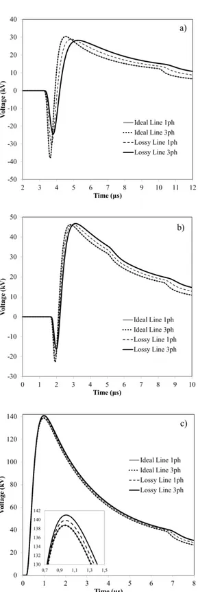
In Figure 1-26, a comparison between the induced voltages at the termination of a 5-km long, single conductor line (configuration a) evaluated with the Rachidi et al. formula and the proposed one is shown. The results associated with the case of an ideal (lossless) line are also presented. The attenuation effect of the transient ground resistance evaluated with the proposed formula is somewhat stronger compared to that obtained using the Rachidi et al. one. Specifically, the negative peak of the overvoltage predicted by the proposed formula is 11% lower than the one obtained using Rachidi et al. formula. In addition, the maximum value of the time derivative of the induced voltage evaluated making use of the proposed approach is 22% lower than with the use
of Rachidi et al. formula, and the rise time is 4% larger. In Figure 1-27, the same comparison is shown for a three-phase line (configuration b in Figure 1-24). While the induced voltage on an ideal line is not affected by the presence of the other conductors (Napolitano et al., 2015), the effect of the mutual transient ground resistance matrix elements is to increase the attenuation effect on the overvoltage. For the assumed configuration, the increasing of the number of conductors leads to a more significant difference between the two formulae in terms of time derivative and peak value of the overvoltage.
Figure 1-25 – Induced voltage at the end of the line. Comparison between the proposed formula (analytical) and the numerical evaluation of the transient ground resistance. 5-km long line, σg =10-3 S/m, εrg = 10.
Figure 1-26 – Induced voltage at the end of the line. Comparison between the proposed formula and the Rachidi et al. one. The results associated with a lossless (ideal) line are also shown for comparison. Single-conductor, 5-km long line, σg =10-3 S/m, εrg = 10.
Figure 1-27 – Induced voltage at the end of the line. Comparison between the proposed formula and the Rachidi et al. one. The results associated with a lossless (ideal) line are also shown for comparison. Three-phase, 5-km long line, σg
=10-3 S/m, εrg = 10.
The main factors that influence the difference between the proposed formulation and the Rachidi
et al. one are the following:
− Ground conductivity and relative permittivity
In Figure 1-28, a comparison between the induced voltage at the termination of a 5-km long single-conductor line evaluated with the Rachidi et al. formula and the proposed algorithm is shown for the case of a ground conductivity σg =10-4 S/m. In this case, the voltage peak calculated with the new approach is 16% lower, the rise-time is 24% larger and the maximum time derivative is 37% lower. The lower the ground conductivity, the higher will be the difference between the two formulations. Opposite consideration can be drawn for the relative ground permittivity; an increase of the ground permittivity leads to more significant differences between the two formulations.
Figure 1-28 – Induced voltage at the end of the line. Comparison between the proposed formula and the Rachidi et al. one. Single-conductor, 5-km long line, σg =10-4 S/m, εrg = 10.
− Current derivative
In Figure 1-29, the same case of Figure 1-25 (shown in black) is compared with the case in which the overvoltages are evaluated assuming three different channel-base current waveforms, having same current peak amplitude of 12 kA and three different maximum time derivative, specifically 12 and 120 kA/μs instead of 40 kA/μs. The currents are named A1, A2 and A3, respectively. Current A2, that is the one adopted in the calculation previously shown, is assumed as representative of a subsequent return stroke. The Heidler functions parameters reported in (Guerrieri et al., 1996) are adopted. For given values of the ground parameters, as the steepness of the electromagnetic source increases, the differences between the two formulation increase. A summary of the previous considerations is reported in Table 1-2. The values are reported in relative value respect to the Rachidi et al. formula. As Table 1-2 shows, significant differences in peak and maximum steepness can be found also for a ground conductivity of 2 mS/m when dealing with fast electromagnetic sources. In view of this, the adoption of the proposed approach is advisable when the ground conductivity is less or equal to 2 mS/m.
Figure 1-29 – Induced voltage at the end of the line. Comparison between the proposed formula and the Rachidi et al. one for the three different return stroke current A1, A2 and A3. Single-conductor, 5-km long line, σg =10-3 S/m, εrg =
TABLE 1-2– INDUCED VOLTAGES – DIFFERENCES BETWEEN THE TWO APPROACHES
σg (mS/m) Current Peak Raise-Time (dV/dt)max
2 A1 A2 -1% -7% 3% 4% -14% -6% A3 -9% 5% -17% 1 A1 -3% 8% -12% A2 -11% 4% -22% A3 -14% 9% -25% A2 3phase -12% 17% -30% 0.1 A1 A2 -16% -9% 14% 24% -26% -37% A3 -19% 26% -39%
− Length of the line
An increase of the length of the line would generally lead to more significant differences between overvoltages calculated using the two different formulae.
Other factors such as the height of the line, the stroke location and the number of conductors have, in general, a minor influence on the difference between the two discussed formulae.
Let us finally discuss the impact of using different approaches to calculate the transient ground resistance on induced voltages considering also a line including a conductor with multiple ground terminations. In this respect, let us make reference to configuration b of Figure 1-24 with the presence of a fourth conductor located under the central phase, at 8.37 m above ground, with multiple groundings every 200 m with resistance equal to 50 Ω. The line is 4 km long with open terminations and the stroke location is 50 m far from the line. The base channel current waveform is the one suggested in (Cigré Working Group 33.01, 1991) to represent a typical negative first-stroke with current peak Ip = 31 kA, equivalent front time tF = 3 μs, maximum steepness Sm = 26
kA/μs and time to half value th = 75 μs. The ground conductivity is σg = 10-4 S/m. In Figure 1-30,
the overvoltage on the central conductor calculated at the line termination is reported for the two different methods. The first negative peak is about 15% lower in case the proposed formula is adopted; the differences between the two waveforms increase with time due to the subsequent traveling wave reflections. Such differences are expected to be more significant if lower tF or
Figure 1-30 – Induced voltage at the end of the line. Comparison between the proposed formula and the Rachidi et al. Three-conductor, 4-km long line, with neutral grounded every 200 m. σg =10-4 S/m, εrg = 10.
Conclusion
A new analytical approach for the evaluation of the transient ground resistance matrix of an overhead multiconductor line above a lossy ground has been proposed. The approach adopts an early-time analytical formula derived from the inverse Laplace transform of the Sunde logarithmic expression of the ground impedance matrix and the late time inverse transforms of Carson formula proposed by Timotin and Orzan. It has been proven that the proposed formula is not affected by any singularity at the early times, contrary to the previously proposed low frequency expressions such as the one by Timotin and its derivations. The proposed approach has been used for the evaluation of lightning-induced transients along a multi-conductor line. In order to show the advantages of the proposed formulation with respect to others recently proposed aimed at fixing the low frequency singularity, a comparison between the overvoltages induced on a lossy line according to the approach used by Rachidi et al., with those calculated using the proposed approach has been carried out. It was shown that for fast electromagnetic sources, and/or poor ground conductivities, the proposed expression provides more accurate results compared to the approach used by Rachidi et al.
1.3.2. Inverse Laplace Transform of Sunde’s Logarithmic Formula – The
Integral Expression
In this section the sum of the series proposed in (Tossani et al., 2015b) is achieved and to this purpose a new formula for the assessment of the transient ground resistance matrix of a multiconductor overhead line is proposed. This new formula is the integral of the difference
between a modified Struve function and a modified Bessel function, of order –1 and 1 respectively, over a finite interval.
The expression proposed by Sunde for the diagonal elements of the ground impedance matrix is (Sunde, 1968) 0 , 1 ( ) ln 2 g i g ii g i h s Z s h γ µ π γ + ¢ = (1.34)
where hi is the height of the i-th conductor and γgis the wave propagation constant above a
finitely conducting ground characterized by its conductivity σg and its relative permittivity εrg,
defined as
(
)
0 0
g s g s rg
γ = µ σ + ε ε (1.35)
The diagonal elements of the transient ground resistance matrix are defined as the inverse Laplace transform of (1.34) divided by s, and are given by (Tossani et al., 2015b)
( )
1 1 2 1 0 2 2 , 1 2 1 ( ) e 1 2 2 n n at n g ii n n i at I t t n a nb µ π ξ π Γ - -¥ - + = æ ö÷ ç ÷ ç ÷ çè ø æ ö÷ ç ¢ = - ç ÷çè ø÷ æ ö ÷ ç ÷ ç ÷ çè øå
(1.36) where a=σ ε εg 0 rg, bi =hi µ ε ε0 0 rg .According to (Gustav Doetsch, 1974) theorem 30.1, the series (1.36) is the inverse Laplace transform of (1.34) in the half plane of convergence defined by hiγg >1 and it converges absolutely for any real time t ≥ 0.
Using the recurrence formula for the Gamma function one gets
1 3 ( 1) 2 2 2 k k k Γçæç + ö÷÷÷ + = ×Γæçç + ÷÷ö÷ ç ç è ø è ø (1.37)
which substituted in (1.36) yields to
( )
2 0 2 2 , 2 0 2 ( ) e 1 3 2 2 2 k k at k g ii k i i at I t t k b ab µ π ξ π Γ ¥ -= æ ö÷ ç ÷ ç ÷ ç æ ö÷ è ø ç ¢ = - çç ÷÷÷ æ ö ç + è ø ç ÷÷ ç ÷ çè øå
(1.38)(
)
0 2 , ( ) e 1 2 2 2 at g ii i t S S b µ π ξ π -¢ = - (1.39) where 1 2 0 2 3 2 k k k at I t S ab k Γ ¥ = æ ö÷ ç ÷ ç ÷ ç æ ö÷ è ø ç = ççè ÷÷ø æ ö ÷ ç + ÷ ç ÷ çè øå
(1.40) and(
)
1/2 1/2 2 2 0 2 2 k k k at I t S k ab Γ + + ¥ = æ ö÷ ç ÷ ç ÷ ç æ ö÷ è ø ç =å
ççè ÷÷ø + (1.41)Let us now substitute the integral definition of the modified Bessel function of real order (see (Abramowitz & Stegun, 1964) equation 9.6.18) in both (1.40) and (1.41). For the first series we obtain 2 cos 2 1 0 0 sin 1 2 e 3 1 2 2 k at x k t x b S dx k k π π Γ Γ ¥ = æ ö÷ ç ÷ ç ÷ çè ø = æ ö æ ö ÷ ÷ ç + ÷ ç + ÷ ç ÷ ç ÷ ç ç è ø è ø
å
ò
(1.42)while for the second one
(
)
2 1 cos 2 2 0 0 sin 1 2 e ! 2 k at x k t x b S dx k k π π Γ + ¥ = æ ö÷ ç ÷ ç ÷ çè ø = +å
ò
(1.43)By using the series definition of the modified Struve function L-1and that of the modified Bessel function I1 in (1.42) and (1.43) respectively (see (Abramowitz & Stegun, 1964) equations 9.6.10 and 12.2.1), one obtains the following expression for the diagonal elements of the transient ground resistance matrix
(cos 1) 0 2 , 1 1 0 ( ) sin sin 4 at x g ii i t t t x I x e dx b b b π µ ξ π -é æç ö÷ æç ö÷ù ê ú ¢ = ê èçç ÷÷ø- èçç ÷ø÷ú ë û
ò
L (1.44)The off-diagonal elements of the transient ground resistance matrix are given by (Tossani et al., 2015b)
( )
( )
1 1 2 1 0 2 2 , 1 cos 2 ( ) e 1 2 ˆ 2 n n at m n ij g ij n n ij at I n t t n a n b δ µ π ξ π Γ - -- + = æ ö÷ ç ÷ ç ÷ çè ø æ ö÷ ç ¢ = - ç ÷çè ø÷ æ ö ÷ ç ÷ ç ÷ çè øå
(1.45)where, being the height of the conductors hi and hj and their mutual distance rij , we have
0 0 ˆ 2 2 i j ij ij rg h h r b = µ ε ε æççç + + j ö÷÷÷ ÷ çè ø and δij =Arg b
( )
ˆij .Following the same procedure adopted for the diagonal elements we can express (1.45) as
(cos 1) 0 2 , 1 1 0 ( ) Re sin sin ˆ ˆ ˆ 4 ij ij ij j j j at x g ij ij ij ij e te te t x I x e dx b b b π δ δ δ µ ξ π -ü é ù ì æ ö æ ö ï ï ç ÷ ç ÷ ï ï ê ç ÷ ç ÷ú ï ï ÷ ÷ ï ¢ = í ê çç ÷÷- çç ÷÷ú ý ê ú ï ç ÷ ç ÷ ï ï ê çè ÷ø çè ÷øú ï ï ï î ë û ïþ
ò
L (1.46)Considering that δij is, in general, small for realistic configurations of distributions and
transmission lines, to avoid unessential complexities (i.e. the presence of complex arguments in the integrand), the following approximation is proposed
(cos 1) 0 2 , 1 1 0 cos ( ) sin sin ˆ ˆ ˆ 4 at x ij g ij ij ij ij t t t x I x e dx b b b π δ µ ξ π -é æç ö÷ æç ö÷ù ê ç ÷÷ ç ÷÷ú ¢ » ê çç ÷÷- çç ÷÷ú ê çç ÷÷ çç ÷÷ú ê è ø è øú ë û
ò
L (1.47)Let us now discuss the behavior of the integrand in (1.44) and (1.47). Many accurate approximations for the evaluation of the modified Struve function are available such as (Luke, 1975; Newman, 1984; Allan J. Macleod, 1993). However, the evaluation of L-1-I1 by separate computation of the Bessel and Struve functions leads to severe cancellation problems. In (Allan J.
Macleod, 1993) the evaluation of L-1-I1 is carried out by using Chebyshev expansions and the coefficients are derived to an accuracy of 20D. The same author proposes in (Allan J. Macleod, 1996) an algorithm for evaluating a Chebyshev series, using the Clenshaw method with Reinsch modification, as analyzed in (Oliver, 1977). We here make use of the coefficients given in (Allan J.
Macleod, 1993) and the algorithm in (Allan J. Macleod, 1996) to calculate our integrand by using
the following relation
1 1
2 π
- = +