CISE, University of Florida Gainesville, FL, USA
https://orcid.org/0000-0001-9509-9725
Travis Gagie
2EIT, Diego Portales University Santiago, Chile
1exCeBiB Santiago, Chile
https://orcid.org/0000-0003-3689-327X
Alan Kuhnle
3CISE, University of Florida Gainesville, FL, USA
https://orcid.org/0000-0001-6506-1902
Giovanni Manzini
4University of Eastern Piedmont Alessandria, Italy
1exIIT, CNR Pisa, Italy
https://orcid.org/0000-0002-5047-0196
Abstract
High-throughput sequencing technologies have led to explosive growth of genomic databases; one of which will soon reach hundreds of terabytes. For many applications we want to build and store indexes of these databases but constructing such indexes is a challenge. Fortunately, many of these genomic databases are highly-repetitive – a characteristic that can be exploited and enable the computation of the Burrows-Wheeler Transform (BWT), which underlies many popular indexes. In this paper, we introduce a preprocessing algorithm, referred to as prefix-free
parsing, that takes a text T as input, and in one-pass generates a dictionary D and a parse P
of T with the property that the BWT of T can be constructed from D and P using workspace proportional to their total size and O(|T |)-time. Our experiments show that D and P are significantly smaller than T in practice, and thus, can fit in a reasonable internal memory even when T is very large. Therefore, prefix-free parsing eases BWT construction, which is pertinent to many bioinformatics applications.
2012 ACM Subject Classification Theory of computation → Design and analysis of algorithms
Keywords and phrases Burrows-Wheeler Transform, prefix-free parsing, compression-aware al-gorithms, genomic databases
Digital Object Identifier 10.4230/LIPIcs.WABI.2018.2
1 Partially supported by National Science Foundation grant 1618814. 2 Partially supported by FONDECYT grant 1171058.
3 Partially supported by National Science Foundation grant 1618814 and a post-doctoral fellowship from
the University of Florida Informatics Institute.
4 Partially supported by PRIN grant 201534HNXC
© Christina Boucher, Travis Gagie, Alan Kuhnle, and Giovanni Manzini; licensed under Creative Commons License CC-BY
Supplement Material Source code: https://gitlab.com/manzai/Big-BWT
Acknowledgements The authors thank Risto Järvinen for the insight they gained from his pro-ject on rsync in the Data Compression course at Aalto University.
1
Introduction
The money and time needed to sequence a genome have shrunk shockingly quickly and researchers’ ambitions have grown almost as quickly: the Human Genome Project cost billions of dollars and took a decade but now we can sequence a genome for about a thousand dollars in about a day. The 1000 Genomes Project [21] was announced in 2008 and completed in 2015, and now the 100,000 Genomes Project is well under way [22]. With no compression 100,000 human genomes occupy roughly 300 terabytes of space, and genomic databases will have grown even more by the time a standard research machine has that much RAM. At the same time, other initiatives have began to study how microbial species behave and thrive in environments. These initiatives are generating public datasets which are just are as equally challenging from a size perspective as the 100,000 Genomes Project. For example, in recent years, there has been an initiative to move toward using whole genome sequencing to accurately identify and track foodborne pathogens (e.g. antibiotic resistant bacteria) [5]. This led to the existence of GenomeTrakr, which is a large public effort to use genome sequencing for surveillance and detection of outbreaks of foodborne illnesses. Currently, the GenomeTrakr effort includes over 100,000 samples, spanning several species available through this initiative – a number that continues to rise as datasets are continually added [19]. Unfortunately, analysis of this data is limited due to their size, even though the similarity between genomes of individuals of the same species means the data is highly compressible.
These public databases are used in various applications – e.g., to detect genetic variation within individuals, determine evolutionary history within a population, and assemble the genomes of novel (microbial) species or genes. Pattern matching within these large databases is fundamental to all these applications, yet repeatedly scanning these – even compressed – databases is infeasible. Thus for these and many other applications, we want to build and use indexes from the database. Since these indexes should also fit in RAM and cannot rely on word boundaries, there are only a few candidates. Many of the popular indexes in bioinformatics are based on the Burrows-Wheeler Transform (BWT) [4] and there have been a number of papers about building BWTs for genomic databases; see, e.g., [18] and references therein. However, it is difficult to process anything more than a few terabytes of raw data per day with current techniques and technology because of the difficulty of working in external memory.
Since genomic databases are often highly repetitive, we revisit the idea of applying a simple compression scheme and then computing the BWT from the resulting encoding in internal memory. This is far from being a novel idea – e.g., Ferragina, Gagie and Manzini’s bwtdisk software [7] could already in 2010 take advantage of its input being given compressed, and Policriti and Prezza [17] recently showed how to compute the BWT from the LZ77 parse of the input using O(n(log r + log z))-time and O(r + z)-space, where n is the length of the uncompressed input, r is the number of runs in the BWT and z is the number of phrases in the LZ77 parse – but we think the preprocessing step we describe here, prefix-free parsing, stands out because of its simplicity and flexibility. Specifically, the parsing algorithm itself is straightforward and it can either be made to work using a single pass over the data on disk or it can be parallelized. Once we have the results of the parsing, which are a dictionary
and a parse, building the BWT out of them is more involved, but when our approach works well, the dictionary and the parse are together much smaller than the initial dataset and that makes the BWT computation less resource-intensive.
Our Contributions. In this paper, we formally define and present prefix-free parsing. The main idea of this method is to divide the input text into overlapping variable-length phrases with delimiting prefixes and suffixes. To accomplish this division, we slide a window of length w over the text and, whenever the Karp-Rabin hash of the window is 0 modulo p, we terminate the current phrase at the end of the window and start the next one at the beginning of the window. This concept is partly inspired by rsync’s [1] use of a rolling hash for content-slicing. Here, w and p are parameters that affect the size of the dictionary of distinct phrases and the number of phrases in the parse. This takes linear-time and one pass over the text, or it can be sped up by running several windows in different positions over the text in parallel and then merging the results.
Just as rsync can usually recognize when most of a file remains the same, we expect that for most genomic databases and good choices of w and p, the total length of the phrases in the dictionary and the number of phrases in the parse will be small in comparison to the uncompressed size of the database. We demonstrate experimentally that with prefix-free parsing we can compute BWT using less memory and equivalent time. In particular, using our method we reduce peak memory usage up to 10x over a standard baseline algorithm which computes the BWT by first computing the suffix array using the algorithm SACA-K [16], while requiring roughly the same time on large sets of salmonella genomes obtained from GenomeTrakr.
In Section 3, we show how we can compute the BWT of the text from the dictionary and the parse alone using workspace proportional only to their total size, and time linear in the uncompressed size of the text when we can work in internal memory. In Section 4 we describe our implementation and report the results of our experiments showing that in practice the dictionary and parse often are significantly smaller than the text and so may fit in a reasonable internal memory even when the text is very large, and that this often makes the overall BWT computation both faster and smaller. We conclude in Section 5 and discuss directions for future work. Prefix-free parsing and all accompanied documents are available at https://gitlab.com/manzai/Big-BWT.
2
Review of the Burrows-Wheeler Transform
As part of the Human Genome Project, researchers had to piece together a huge number of relatively tiny, overlapping pieces of DNA, called reads, to assemble a reference genome about which they had little prior knowledge. Once the Project was completed, however, they could then use that reference genome as a guide to assemble other human genomes much more easily. To do this, they indexed the reference genome such that, after running a DNA sample from a new person through a sequencing machine and obtaining another collection of reads, for each of those new reads they could quickly determine which part of the reference genome it matched most closely. Since any two humans are genetically very similar, aligning the new reads against the reference genome gives a good idea of how they are really laid out in the person’s genome.
In practice, the best solutions to this problem of indexed approximate matching work by reducing it to a problem of indexed exact matching, which we can formalize as follows: given a string T (which can be the concatenation of a collection of strings, terminated by
19 27 9 17 $1 T A C $1 $2 $3 26 2 3 4 5 16 15 14 $1 T A C $1 T A C $1 $1 6 $1 7 $1 8 $1 10 $2 T A C 1 $2 T A C 11 12 $2 13 $2 $2 $2 $2 T A G 18 $3 A T A G $3 A 20 T A G $3 A 21 T A G $3 A 22 T A G $3 A 24 25 $3 23 $3 $3 $3 T A C A A T T A T A C A T A T A G A T A C T T A G A T A C A T $2 10 11 12 13 14 15 16 17 G A T T A C A T $1 1 2 3 4 5 6 7 8 9 G A T T A G A T A $3 18 19 20 21 22 23 24 25 26 27
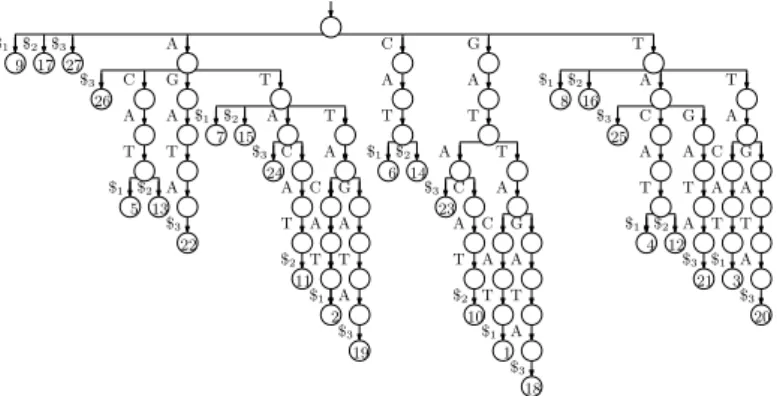
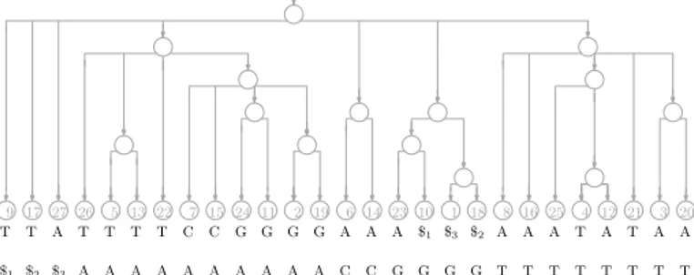
Figure 1 The suffix trie for our example with the three strings GATTACAT, GATACAT and
GATTAGATA. The input is shown at the bottom, in grey because we do not need to store it.
special symbols), pre-process it such that later, given a pattern P , we can quickly list all the locations where P occurs in T . We now start with a simple but impractical solution to the latter problem, and then refine it until we arrive at a fair approximation of the basis of most modern assemblers, illustrating the workings of the Burrows-Wheeler Transform (BWT) along the way.
Suppose we want to index the three strings GATTACAT, GATACAT and GATTAGATA, so T [1..n] = GATTACAT$1GATACAT$2GATTAGATA$3, where $1, $2and $3 are termin-ator symbols. Perhaps the simplest solution to the problem of indexing T is to build a trie of the suffixes of the three strings in our collection (i.e., an edge-labelled tree whose root-to-leaf paths are the suffixes of those strings) with each leaf storing the starting position of the suffix labelling the path to that leaf, as shown in Figure 1.
Suppose every node stores pointers to its children and its leftmost and rightmost leaf descendants, and every leaf stores a pointer to the next leaf to its right. Then given P [1..m], we can start at the root and descend along a path (if there is one) such that the to the node at depth i is P [i], until we reach a node v at depth m + 1. We then traverse the leaves in v’s subtree, reporting the the starting positions stored at them, by following the pointer from v to its leftmost leaf descendant and then following the pointer from each leaf to the next leaf to its right until we reach v’s rightmost leaf descendant.
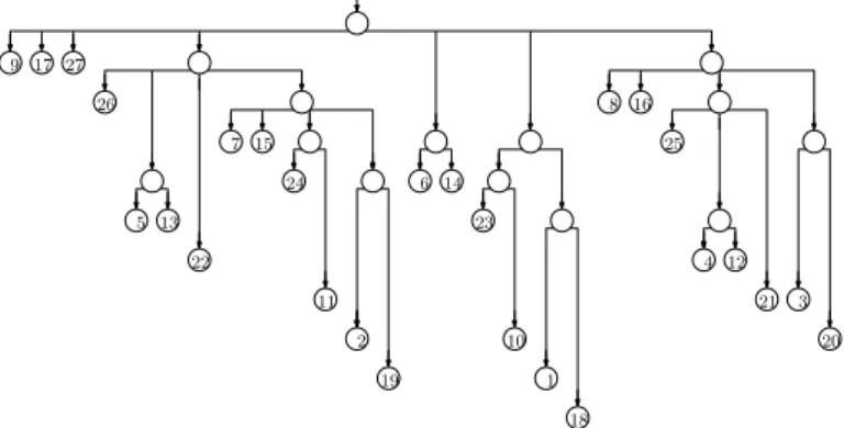
The trie of the suffixes can have a quadratic number of nodes, so it is impractical for large strings. If we remove nodes with exactly one child (concatenating the edge-labels above and below them), however, then there are only linearly many nodes, and each edge-label is a substring of the input and can be represented in constant space if we have the input stored as well. The resulting structure is essentially a suffix tree (although it lacks suffix and Weiner links), as shown in Figure 2. Notice that the label of the path leading to a node v is the longest common prefix of the suffixes starting at the positions stored at v’s leftmost and rightmost leaf descendants, so we can navigate in the suffix tree, using only the pointers we already have and access to the input.
Although linear, the suffix tree still takes up an impractical amount of space, using several bytes for each character of the input. This is significantly reduced if we discard the shape of the tree, keeping only the input and the starting positions in an array, which is called the
19 27 9 17 26 2 3 4 5 16 15 14 6 7 8 10 1 11 12 13 18 20 21 22 24 25 23 G A T A C A T $2 10 11 12 13 14 15 16 17 G A T T A C A T $1 1 2 3 4 5 6 7 8 9 G A T T A G A T A $3 18 19 20 21 22 23 24 25 26 27
Figure 2 The suffix tree for our example. We now store the input.
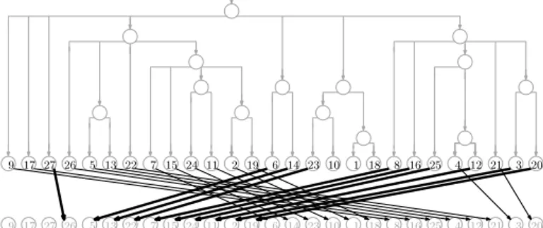
suffix array (SA). The SA for our example is shown in Figure 3. Since the entries of the SA are the starting points of the suffixes in lexicographic order, with access to T we can perform two binary searchs to find the endpoints of the interval of the suffix array containing the starting points of suffixes starting with P : at each step, we consider an entry SA[i] and check if T [SA[i]] lexicographically precedes P . This takes a total of O(m log n) time done naïvely, and can be sped up with more sophisticated searching and relatively small auxiliary data structures.
Even the SA takes linear space, however, which is significantly more than what is needed to store the input when the alphabet is small (as it is in the case of DNA). Let Ψ be the function that, given the position of a value i < n in the SA, returns the position of i + 1. Notice that, if we write down the first character of each suffix in the order they appear in the SA, the result is a sorted list of the characters in T , which can be stored using using O(log n) bits for each character in the alphabet. Once we have this list stored, given a position i in SA, we can return T [SA[i]] efficiently.
Given a position i in SA and a way to evaluate Ψ, we can extract T [SA[i]..n] by writing T [SA[i]], T [SA[Ψ(i)]], T [SA[Ψ2(i)]], . . .. Therefore, we can perform the same kind of binary search we use when with access to a full suffix array. Notice that if T [SA[i]] ≺
T [SA[i + 1]] then Ψ(i) < Ψ(i + 1), meaning that Ψ(1), . . . , Ψ(n) can be divided into σ
increasing consecutive subsequences, where σ is the size of the alphabet. It follows that we can store nH0(T ) + o(n log σ) bits, where H0(T ) is the 0th-order empirical entropy of T , such that we can quickly evaluate Ψ. This bound can be improved with a more careful analysis. Now suppose that instead of a way to evaluate Ψ, we have a way to evaluate quickly its inverse, which is called the last-to-first (LF) mapping. (This name was not chose because, if we start with the position of n in the suffix array and repeatedly apply the LF mapping we enumerate the positions in the SA in decreasing order of their contents, ending with 1; to some extent, the name is a lucky coincidence.) The LF mapping for our example is also shown with arrows in Figure 3. Since it is the inverse of Ψ, the sequence LF(1), . . . , LF(n) can be partitioned into σ incrementing subsequences: for each character c in the alphabet, if the starting positions of suffixes preceded by copies of c are stored in SA[j1], . . . , SA[jt] (appearing in that order in the SA), then LF(j1) is 1 greater than the number of characters
18 27 9 17 26 5 13 22 7 15 24 11 2 19 6 14 23 10 1 8 16 25 4 12 21 3 20 18 27 9 17 26 5 13 22 7 15 24 11 2 19 6 14 23 10 1 8 16 25 4 12 21 3 20 G A T A C A T $2 10 11 12 13 14 15 16 17 G A T T A C A T $1 1 2 3 4 5 6 7 8 9 G A T T A G A T A $3 18 19 20 21 22 23 24 25 26 27
Figure 3 The suffix array for our example is the sequence of values stored in the leaves of the
tree (which we need not store explicitly). The LF mapping is shown as the arrows between two copies of the suffix array; the arrows to values i such that T [SA[i]] = A are heavy, to illustrate that they point to consecutive positions in the suffix array and do not cross. Since Ψ is the inverse of the LF mapping, it can be obtained by simply reversing the direction of the arrows.
lexicographically less than c in T and LF(j2), . . . , LF(jt) are the next t − 1 numbers. Figure 3 illustrates this, with the arrows to values i such that T [SA[i]] = A heavy, to illustrate that they point to consecutive positions in the suffix array and do not cross.
Consider the interval IP [i..m] of the SA containing the starting positions of suffixes beginning with P [i..m], and the interval IP [i−1]containing the starting positions of suffixes beginning with P [i − 1]. If we apply the LF mapping to the SA positions in IP [i..m], the SA positions we obtain that lie in IP [i−1]for a consecutive subinterval, containing the starting positions in T of suffixes beginning with P [i − 1..m]. Therefore, we can search also with the LF mapping.
If we write the character preceding each suffix of T (considering it to be cyclic) in the lexicographic order of the suffixes, the result is the Burrows-Wheeler Transform (BWT) of
T . A rank data structure over the BWT (which, given a character and a position, returns
the number of occurrences of that character up to that position) can be used to implement searching with the LF-mapping, together with an array C indicating for each character in the alphabet how many characters in T are lexicographically strictly smaller than it. Specifically,
LF(i) = BWT.rankBWT[i](i) + C[BWT[i]] .
If follows that, to compute IP [i−1..m] from IP [i..m], we perform a rank query for P [i − 1] immediately before the beginning of IP [i..m] and add C[P [i + 1]] + 1 to the result, to find the beginning of IP [i−1..m]; and we perform a rank query for P [i − 1] at the end of IP [i..m] and add C[P [i + 1]] to the result, to find the end of IP [i−1..m]. Figure 4 shows the BWT for our example, and the sorted list of characters in T . Comparing it to Figure 3 makes the formula above clear: if BWT[i] is the jth occurrence of that character in the BWT, then the arrow from LF(i) leads from i to the position of the jth occurrence of that character in the sorted list. This is the main idea behind FM-indexes [8], and the main motivation for bioinformaticians to be interested in building BWTs.
18 27 9 17 26 5 13 22 7 15 24 11 2 19 6 14 23 10 1 8 16 25 4 12 21 3 20 18 27 9 17 26 5 13 22 7 15 24 11 2 19 6 14 23 10 1 8 16 25 4 12 21 3 20 $3 $1 $2 T T A T T T T C C G G G G A A A A A A T A T A A $1 $2 $3 A A A A A A A A A A C C G G G G T T T T T T T T G A T A C A T $2 10 11 12 13 14 15 16 17 G A T T A C A T $1 1 2 3 4 5 6 7 8 9 G A T T A G A T A $3 18 19 20 21 22 23 24 25 26 27
Figure 4 The BWT and the sorted list of characters for our example. Drawing arrows between
corresponding occurrences of characters in the two strings gives us the diagram for the LF-mapping.
3
Theory
We let E ⊆ Σw be any set of strings each of length w ≥ 1 over the alphabet Σ and let
E0= E ∪ {#, $w}, where # and $ are special symbols lexicographically less than any in Σ. We consider a text T [0..n − 1] over Σ and let D be the maximum set such that for d ∈ D,
d is a substring of # T $w,
exactly one proper prefix of d is in E0, exactly one proper suffix of d is in E0, no other substring of d is in E0.
We let S be the set of suffixes of length greater than w of elements of D.
Given T and a way to recognize strings in E, we can build D iteratively by simulating scanning # T $wto find occurrences of elements of E0, adding to D each substring of # T $w that starts at the beginning of one such occurrence and ends at the end of the next one. While we are building D we also build a list P of the occurrences of the elements of D in T , which we call the parse (although each consecutive pair of elements overlap by w characters, so P is not a partition of the characters of # T $w). We then build S from D and sort it.
For example, suppose we have Σ = {!, A, C, G, T}, w = 2, E = {AC, AG, T!} and
T = GATTACAT!GATACAT!GATTAGATA .
Then it follows that we get
D = {#GATTAC, ACAT!, AGATA$$, T!GATAC, T!GATTAG} ,
S = {#GATTAC, GATTAC, . . . , TAC, ACAT!, CAT!, AT!,
AGATA$$, GATA$$, . . . , A$$, T!GATAC, !GATAC, . . . , TAC, T!GATTAG, !GATTAG, . . . , TAG}
ILemma 1. S is a prefix-free set.
Proof. If s ∈ S were a proper prefix of s0∈ S then, since |s| > w, the last w characters of s – which are an element of E0 – would be a substring of s0 but neither a proper prefix nor a proper suffix of s0. Therefore, any element of D with s0 as a suffix would contain at least three substrings in E0, contrary to the definition of D. J I Lemma 2. Suppose s, s0 ∈ S and s ≺ s0. Then sx ≺ s0x0 for any strings x, x0 ∈ (Σ ∪ {#, $})∗.
Proof. By Lemma 1, s and s0 are not proper prefixes of each other. Since they are not equal either (because s ≺ s0), it follows that sx and s0x0 differ on one of their first min(|s|, |s0|)
characters. Therefore, s ≺ s0 implies sx ≺ s0x0. J
ILemma 3. For any suffix x of # T $w with |x| > w, exactly one prefix s of x is in S.
Proof. Consider the substring d stretching from the beginning of the last occurrence of an element of E0 that starts before or at the starting position of x, to the end of the first occurrence of an element of E0 that starts strictly after the starting position of x. Regardless of whether d starts with # or another element of E0, it is prefixed by exactly one element of
E0; similarly, it is suffixed by exactly one element of E0. It follows that d is an element of D. Let s be the prefix of x that ends at the end of that occurrence of d in # T $w, so |s| > w and is a suffix of an element of D and thus s ∈ S. By Lemma 1, no other prefix of x is in S. J Let f be the function that maps each suffix x of # T $wwith |x| > w to the unique prefix
s of x with s ∈ S.
ILemma 4. Let x and x0 be suffixes of # T $w with |x|, |x0| > w. Then f (x) ≺ f (x0) implies
x ≺ x0.
Proof. By the definition of f , f (x) and f (x0) are prefixes of x and x0 with |f (x)|, |f (x0)| > w.
Therefore, f (x) ≺ f (x0) implies x ≺ x0 by Lemma 2. J
Define T0[0..n] = T $. Let g be the function that maps each suffix y of T0 to the unique suffix x of # T $w that starts with y, except that it maps T0[n] = $ to # T $w. Notice that
g(y) always has length greater than w, so it can be given as an argument to f .
ILemma 5. The permutation that lexicographically sorts T [0..n−1] $w, . . . , T [n−1] $w, # T $w also lexicographically sorts T0[0..n], . . . , T0[n − 1..n], T0[n].
Proof. Appending copies of $ to the suffixes of T0 does not change their relative order, and just as # T $wis the lexicographically smallest of T [0..n − 1] $w, . . . , T [n − 1] $w, # T $w, so
T0[n] = $ is the lexicographically smallest of T0[0..n], . . . , T0[n − 1..n], T0[n]. J Let β be the function that, for i < n, maps T0[i] to the lexicographic rank of f (g(T0[i + 1..n])) in S, and maps T [n] to the lexicographic rank of f (g(T0)) = f (T $w).
ILemma 6. Suppose β maps k copies of a to s ∈ S and maps no other characters to s, and
maps a total of t characters to elements of S lexicographically less than s. Then the (t + 1)st through (t + k)th characters of the BWT of T0 are copies of a.
Proof. By Lemmas 4 and 5, if f (g(y)) ≺ f (g(y0)) then y ≺ y0. Therefore, β partially sorts the characters in T0 into their order in the BWT of T0; equivalently, the characters’ partial order according to β can be extended to their total order in the BWT. Since every total extension of β puts those k copies of a in the (t + 1)st through (t + k)th positions, they
From D and P , we can compute how often each element s ∈ S is preceded by each distinct character a in # T $wor, equivalently, how many copies of a are mapped by β to the lexicographic rank of s. If an element s ∈ S is a suffix of only one element d ∈ D and a proper suffix of that – which we can determine first from D alone – then β maps only copies of the the preceding character of d to the rank of s, and we can compute their positions in the BWT of T0. If s = d or a suffix of several elements of D, however, then β can map several distinct characters to the rank of s. To deal with these cases, we can also compute which elements of D contain which characters mapped to the rank of s. We will explain in a moment how we use this information.
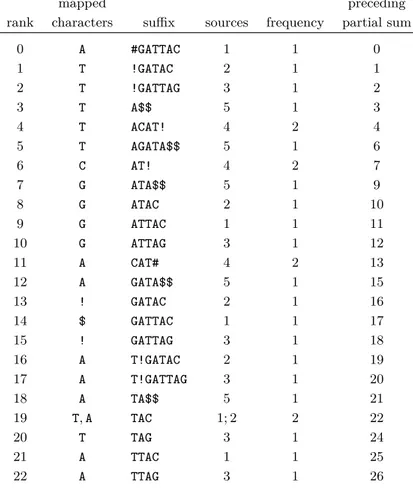
For our example, T = GATTACAT!GATACAT!GATTAGATA, we compute the information shown in Table 1. To ease the comparison to the standard computation of the BWT of T0$, shown in Table 2, we write the characters mapped to each element s ∈ S before s itself.
By Lemma 6, from the characters mapped to each rank by β and the partial sums of frequencies with which β maps characters to the ranks, we can compute the subsequence of the BWT of T0 that contains all the characters β maps to elements of S, which are not complete elements of D and to which only one distinct character is mapped. We can also leave placeholders where appropriate for the characters β maps to elements of S, which are complete elements of D or to which more than one distinct character is mapped. For our example, this subsequence is ATTTTTTCCGGGGAAA!$!AAA - - TAA. Notice we do not need all the infomation in P to compute this subsequence, only D and the frequencies of its elements in P .
Suppose s ∈ S is an entire element of D or a suffix of several elements of D, and occurrences of s are preceded by several distinct characters in # T $w, so β assigns s’s lexicographic rank in S to several distinct characters. To deal with such cases, we can sort the suffixes of the parse P and apply the following lemma.
ILemma 7. Consider two suffixes t and t0 of # T $w starting with occurrences of s ∈ S,
and let q and q0 be the suffixes of P encoding the last w characters of those occurrences of s and the remainders of t and t0. If t ≺ t0 then q ≺ q0.
Proof. Since s occurs at least twice in # T $w, it cannot end with $w and thus cannot be a suffix of # T $w. Therefore, there is a first character on which t and t0 differ. Since the elements of D are represented in the parse by their lexicographic ranks, that character forces
q ≺ q0. J
We consider the occurrences in P of the elements of D suffixed by s, and sort the characters preceding those occurrences of s into the lexicographic order of the remaining suffixes of P which, by Lemma 7, is their order in the BWT of T0. In our example, TAC ∈ S is preceded in # T $$ by a T when it occurs as a suffix of #GATTAC ∈ D, which has rank 0 in
D, and by an A when it occurs as a suffix of T!GATAC ∈ D, which has rank 3 in D. Since the
suffix following 0 in P = 0, 1, 3, 1, 4, 2 is lexicographically smaller than the suffix following 3, that T precedes that A in the BWT.
Since we need only D and the frequencies of its elements in P to apply Lemma 6 to build and store the subsequence of the BWT of T0 that contains all the characters β maps to elements of S, to which only one distinct character is mapped, this takes space proportional to the total length of the elements of D. We can then apply Lemma 7 to build the subsequence of missing characters in the order they appear in the BWT. Although this subsequence of missing characters could take more space than D and P combined, as we generate them we can interleave them with the first subsequence and output them, thus still using workspace proportional to the total length of P and the elements of D and only one pass over the space used to store the BWT.
Table 1 The information we compute for our example, T = GATTACAT!GATACAT!GATTAGATA. Each
line shows the lexicographic rank r of an element s ∈ S; the characters mapped to r by β; s itself; the elements of D from which the mapped characters originate; the total frequency with which characters are mapped to r; and the preceding partial sum of the frequencies.
mapped preceding
rank characters suffix sources frequency partial sum
0 A #GATTAC 1 1 0 1 T !GATAC 2 1 1 2 T !GATTAG 3 1 2 3 T A$$ 5 1 3 4 T ACAT! 4 2 4 5 T AGATA$$ 5 1 6 6 C AT! 4 2 7 7 G ATA$$ 5 1 9 8 G ATAC 2 1 10 9 G ATTAC 1 1 11 10 G ATTAG 3 1 12 11 A CAT# 4 2 13 12 A GATA$$ 5 1 15 13 ! GATAC 2 1 16 14 $ GATTAC 1 1 17 15 ! GATTAG 3 1 18 16 A T!GATAC 2 1 19 17 A T!GATTAG 3 1 20 18 A TA$$ 5 1 21 19 T, A TAC 1; 2 2 22 20 T TAG 3 1 24 21 A TTAC 1 1 25 22 A TTAG 3 1 26
If we want, we can build the first subsequence from D and the frequencies of its elements in P ; store it in external memory; and make a pass over it while we generate the second one from D and P , inserting the missing characters in the appropriate places. This way we use two passes over the space used to store the BWT, but we may use significantly less workspace.
Summarizing, assuming we can recognize the strings in E quickly, we can quickly compute
D and P with one scan over T and then from them, with Lemmas 6 and 7, we can compute
the BWT of T0= T $ by sorting the suffixes of the elements of D and the suffixes of P . Since there are linear-time and linear-space algorithms for sorting suffixes when working in internal memory, this implies our main theoretical result:
ITheorem 8. We can compute the BWT of T $ from D and P using workspace proportional
to sum of the total length of P and the elements of D, and O(n) time when we can work in internal memory.
BWT; the character in that position; and the suffix immediately following that character in T0. i BWT[i] suffix 0 A $ 1 T !GATACAT!GATTAGATA$ 2 T !GATTAGATA$ 3 T A$ 4 T ACAT!GATACAT!GATTAGATA$ 5 T ACAT!GATTAGATA$ 6 T AGATA$ 7 C AT!GATACAT!GATTAGATA$ 8 C AT!GATTAGATA$ 9 G ATA$ 10 G ATACAT!GATTAGATA$ 11 G ATTACAT!GATACAT!GATTAGATA$ 12 G ATTAGATA$ 13 A CAT!GATACAT!GATTAGATA$ 14 A CAT!GATTAGATA$ 15 A GATA$ 16 ! GATACAT!GATTAGATA$ 17 $ GATTACAT!GATACAT!GATTAGATA$ 18 ! GATTAGATA$ 19 A T!GATACAT!GATTAGATA$ 20 A T!GATTAGATA$ 21 A TA$ 22 T TACAT!GATACAT!GATTAGATA$ 23 A TACAT!GATTAGATA$ 24 T TAGATA$ 25 A TTACAT!GATACAT!GATTAGATA$ 26 A TTAGATA$
4
Practice
We have implemented our BWT construction in order to test our conjectures that, first, for most genomic databases and good choices of w and p, the total length of the phrases in the dictionary and the number of phrases in the parse will both be small in comparison to the uncompressed size of the database; second, computing the dictionary and the parse first and then computing the BWT from them leads to an overall speedup and reduction in memory usage. In this section we describe our implementation and then report our experimental results.
4.1
Implementation
As described in Sections 1 and 3, we slide a window of length w over the text, keeping track of the Karp-Rabin hash of the window; we also keep track of the hash of the entire prefix of the current phrase that we have processed so far. Whenever the hash of the window is
0 modulo p, we terminate the current phrase at the end of the window and start the next one at the beginning of the window. We prepend a NULL character to the first phrase and append w copies of NULL to the last phrase. If the text ends with w characters whose hash is 0 modulo p, then we take those w character to be the beginning of the last phrase and append to them w copies of NULL. We note that we prepend and append copies of the same NULL character; although using different characters simplifies the proofs in Section 3, it is not essential in practice.
We keep track of the set of hashes of the distinct phrases in the dictionary so far, as well as the phrases’ frequencies. Whenever we terminate a phrase, we check if its hash is in that set. If not, we add the phrase to the dictionary and its hash to the set, and set its frequency to 1; if so, we compare the current phrase to the one in the dictionary with the same hash to ensure they are equal, then increment its frequency. (Using a 64-bit hash the probability of there being a collision is very low, so we have not implemented a recovery mechanism if one occurs.) In both cases, we write the hash to disk.
When the parsing is complete, we have generated the dictionary D and the parsing
P = p1, p2, . . . , pz, where each phrase pi is represented by its hash. Next, we sort the dictionary and make a pass over P to substitute the phrases’ lexicographic ranks for their hashes. This gives us the final parse, still on disk, with each entry stored as a 4-byte integer. We write the dictionary to disk phrase by phrase in lexicographic order with a special end-of-phrase terminator at the end of each phrase. In a separate file we store the frequency of each phrase in as a 4-byte integer. Using four bytes for each integer does not give us the best compression possible, but it makes it easy to process the frequency and parse files later. Finally, we write to a separate file the array W of length |P | such that W [j] is the character of pj in position w + 1 from the end (recall each phrase has length greater than w). These characters will be used to handle the elements of S that are also elements of D.
Next, we compute the BWT of the parsing P , with each phrase represented by its 4-byte lexicographic rank in D. The computation is done using the SACA-K suffix array construction algorithm [16] which, among the linear time algorithms, is the one using the smallest workspace. Instead of storing BW T (P ) = b1, b2, . . . , bz, we save the same information in a format more suitable for the next phase. We consider the dictionary words in lexicographic order, and, for each word di, we write the list of BWT positions where di appears. We call this the inverted list for word di. Since the size of the inverted list of each word is equal to its frequency, which is available separately, we write to file the plain concatenation of the inverted lists using again four bytes per entry, for a total of 4|P | bytes. In this phase we also permute the elements of W so that now W [j] is the character coming from the phrase that precedes bj in the parsing, i.e. P [SA[j] − 2].
In the final phase of the algorithm we compute the BWT of the input T . We deviate slightly from the description in Section 3 in that instead of lexicographically sorting the suffixes in D larger than w we sort all of them and later ignore those which are of length ≤ w. The sorting is done applying the gSACAK algorithm [14] which computes the SA and LCP array for the set of dictionary phrases. We then proceed as in Section 3. If during the scanning of the sorted set S we meet s which is a proper suffix of several elements of
D we use a heap to merge their respective inverted lists writing a character to the final
BWT file every time we pop a position from the heap. If we meet s which coincides with a dictionary word d we write the characters retrieved from W from the positions obtained from d’s inverted list.
with three settings of the parameters w and p. All sizes are reported in megabytes; percentages are the sums of the sizes of the dictionaries and parses, divided by the sizes of the uncompressed files.
w = 6, p = 20 w = 8, p = 50 w = 10, p = 100
file size dict. parse % dict. parse % dict. parse %
cere 440 61 77 31 43 159 46 89 17 24 cere_no_Ns 409 33 77 27 43 33 18 60 17 19 dna.001.1 100 8 20 27 13 9 21 21 4 25 einstein.en.txt 446 2 87 20 3 39 9 4 17 5 influenza 148 16 28 30 32 12 29 49 6 37 kernel 247 14 52 26 14 20 13 15 10 10 world_leaders 45 5 5 21 8 2 21 11 1 26 world_leaders_no_dots 23 4 5 34 6 2 31 7 1 33
4.2
Experiments
In this section, the parsing and BWT computation are experimentally evaluated. All experiments were run on a server with Intel(R) Xeon(R) CPU E5-2640 v4 @ 2.40GHz and 756 gigabytes of RAM.
Table 3 shows the sizes of the dictionaries and parses for several files from the Pizza & Chili repetitive corpus [2], with three settings of the parameters w and p. We note that cere contains long runs of Ns and world_leaders contains long runs of periods, which can either cause many phrases, when the hash of w copies of those characters is 0 modulo p, or a single long phrase otherwise; we also display the sizes of the dictionaries and parses for those files with all Ns and periods removed. The dictionaries and parses occupy between 5 and 31 percent of the space of the uncompressed files.
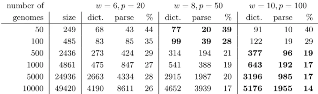
Table 4 shows the sizes of the dictionaries and parses for prefixes of a database of Salmonella genomes [20]. The dictionaries and parses occupy between 14 and 44 percent of the space of the uncompressed files, with the compression improving as the number of genomes increases. In particular, the dataset of ten thousand genomes takes nearly 50 GB uncompressed, but with w = 10 and p = 100 the dictionary and parse take only about 7 GB together, so they would still fit in the RAM of a commodity machine. This seems promising, and we hope the compression is even better for larger genomic databases.
Table 5 shows the runtime and peak memory usage for computing the BWT from the parsing for the database of Salmonella genomes. As a baseline for comparison, simplebwt computes the BWT by first computing the Suffix Array using algorithm SACA-K [16]; SACA-K is a linear time algorithm that uses O(1) workspace and is fast in practice. As shown in Table 5, the peak memory usage of simplebwt is reduced by a factor of 4 to 10 by computing the BWT from the parsing; furthermore, the total runtime is competitive with simplebwt. In some instances, for example the databases of 5000, 10000 genomes, computing the BWT from the parsing achieved significant runtime reduction over simplebwt; with
w = 10, p = 100 on these instances, the runtime reduction is more than factors of 2, 4,
respectively. For our BWT computations, the peak memory usage with w = 6, p = 20 stays within a factor of roughly 2 of the original file size and is smaller than the orginal file size on the larger databases of 1000 genomes. For the database of 5000 genomes, the most expensive steps were parsing and computing the missing characters – about 23% of the total BWT – to fill in the subsequence.
Table 4 The dictionary and parse sizes for prefixes of a database of Salmonella genomes, with
three settings of the parameters w and p. Again, all sizes are reported in megabytes; percentages are the sums of the sizes of the dictionaries and parses, divided by the sizes of the uncompressed files.
number of w = 6, p = 20 w = 8, p = 50 w = 10, p = 100
genomes size dict. parse % dict. parse % dict. parse %
50 249 68 43 44 77 20 39 91 10 40 100 485 83 85 35 99 39 28 122 19 29 500 2436 273 424 29 314 194 21 377 96 19 1000 4861 475 847 27 541 388 19 643 192 17 5000 24936 2663 4334 28 2915 1987 20 3196 985 17 10000 49420 4190 8611 26 4652 3939 17 5176 1955 14
Table 5 Time (seconds) and peak memory consumption (megabytes) of BWT calculations for
prefixes of a database of Salmonella genomes, for three settings of the parameters w and p and for the comparison method simplebwt.
number of w = 6, p = 20 w = 8, p = 50 w = 10, p = 100 simplebwt
genomes time peak time peak time peak time peak
50 71 545 63 642 65 782 53 2247 100 118 709 100 837 102 1059 103 4368 500 570 2519 443 2742 402 3304 565 21923 1000 1155 4517 876 4789 776 5659 1377 43751 5000 7412 42067 5436 46040 4808 51848 11600 224423 10000 19152 68434 12298 74500 10218 84467 43657 444780
Table 6 Time (seconds) and peak memory consumption (megabytes) of BWT calculations on
various files from the Pizza & Chili repetitive corpus, for three settings of the parameters w and p and for the comparison method simplebwt.
w = 6, p = 20 w = 8, p = 50 w = 10, p = 100 simplebwt
file time peak time peak time peak time peak
cere 90 603 79 559 74 801 90 3962
einstein.en.txt 53 196 40 88 35 53 97 4016
influenza 27 166 27 284 33 435 30 1331
kernel 43 170 29 143 25 144 50 2216
world_leaders 7 50 7 74 7 98 7 405
5
Conclusion and Future Work
We have described how prefix-free parsing can be used as preprocessing step to enable compression-aware computation of BWTs of large genomic databases. Our results demonstrate that the dictionaries and parses are often significantly smaller than the original input, and so may fit in a reasonable internal memory even when T is very large. Finally, we show how the BWT can be constructed from a dictionary and parse alone. We plan to investigate using compressed suffix arrays during the construction of the BWT, instead of suffix arrays, which should reduce our memory usage at the cost of increasing the running time by approximately a factor logarithmic in the size of the input; we will report the results in the full version of this paper.
In future extended versions of this work, we plan to explore its applications to sequence datasets that are terabytes in size; such as GenomeTrakr [19] and MetaSub [15]. We note that when downloading large datasets, prefix-free parsing can avoid storing the whole uncompressed dataset in memory or on disk. Suppose we run the parser on the dataset as it is downloaded, either as a stream or in chunks. We have to keep the dictionary in memory for parsing but we can write the parse to disk as we go, and in any case we can use less total space than the dataset itself. Ideally, the parsing could even be done server-side to reduce transmission time and/or bandwidth – which we leave for future implementation and experimentation.
A natural extension of our method is to consider efficient parallelization of the parsing. With k processors, we could divide the input string into k equal blocks, with each consecutive pair of blocks overlapping by w characters; we scan each block with a processor, to find the locations of the substrings of length w with Karp-Rabin hashes congruent to 0 modulo
p; and then we scan the input with the k processors in parallel to compute the dictionary
and parse, starting at roughly evenly-spaced locations of such substrings. Alternatively, our approach can be viewed as a modified Schindler Transform [3] and since previous authors [6] have shown how the Schindler Transform benefits from GPU parallelization, we believe that GPU-based parallelization could be both easy and effective.
Perhaps the main use of BWTs is in FM-indexes [8], which are at the heart of the most popular DNA aligners, including Bowtie [11, 10], BWA [12] and SOAP 2 [13]. With only rank support over a BWT, we can count how many occurrences of a given pattern there are in the text, but we cannot tell where they are without using a suffix-array sample. Until recently, suffix-array samples for massive, highly repetitive datasets were usually either much larger than the datasets BWTs, or very slow. Gagie, Navarro and Prezza [9] have now shown we need only store suffix array values at the ends of runs in the BWT, however, and we conjecture that we can build this sample while computing the BWT from the dictionary and the parse. Indeed, we were initially motivated to study new approaches to BWT construction because without them, Gagie et al.’s result may never realize its full potential.
References
1 rsync. URL: https://rsync.samba.org.
2 Repetitive corpus. URL: http://pizzachili.dcc.uchile.cl/repcorpus.html.
3 The sort transformation. URL: http://www.compressconsult.com/st.
4 Michael Burrows and David J. Wheeler. A block-sorting lossless compression algorithm. Technical report, Digital Equipment Corporation, 1994.
5 H.A. Carleton and P. Gerner-Smidt. Whole-genome sequencing is taking over foodborne disease surveillance. Microbe, 11:311–317, 2016.
6 Chia-Hua Chang, Min-Te Chou, Yi-Chung Wu, Ting-Wei Hong, Yun-Lung Li, Chia-Hsiang Yang, and Jui-Hung Hung. sBWT: memory efficient implementation of the hardware-acceleration-friendly Schindler transform for the fast biological sequence mapping.
Bioin-formatics, 32(22):3498–3500, 2016.
7 Paolo Ferragina, Travis Gagie, and Giovanni Manzini. Lightweight data indexing and compression in external memory. Algorithmica, 63(3):707–730, 2012.
8 Paolo Ferragina and Giovanni Manzini. Indexing compressed text. Journal of the ACM
(JACM), 52(4):552–581, 2005.
9 Travis Gagie, Gonzalo Navarro, and Nicola Prezza. Optimal-time text indexing in bwt-runs bounded space. In Proceedings of the 29th Symposium on Discrete Algorithms (SODA), pages 1459–1477, 2018.
10 Ben Langmead and Steven L Salzberg. Fast gapped-read alignment with Bowtie 2. Nature
Methods, 9(4):357–360, 2012. doi:10.1038/nmeth.1923.
11 Ben Langmead, Cole Trapnell, Mihai Pop, and Steven L Salzberg. Ultrafast and memory-efficient alignment of short DNA sequences to the human genome. Genome biology,
10(3):R25, 2009.
12 Heng Li and Richard Durbin. Fast and accurate long-read alignment with burrows–wheeler transform. Bioinformatics, 26(5):589–595, 2010.
13 Ruiqiang Li, Chang Yu, Yingrui Li, Tak-Wah Lam, Siu-Ming Yiu, Karsten Kristiansen, and Jun Wang. Soap2: an improved ultrafast tool for short read alignment. Bioinformatics, 25(15):1966–1967, 2009.
14 Felipe Alves Louza, Simon Gog, and Guilherme P. Telles. Inducing enhanced suffix arrays for string collections. Theor. Comput. Sci., 678:22–39, 2017.
15 MetaSUB International Consortium. The Metagenomics and Metadesign of the Subways and Urban Biomes (MetaSUB) International Consortium inaugural meeting report.
Micro-biome, 4(1):24, 2016.
16 Ge Nong. Practical linear-time O(1)-workspace suffix sorting for constant alphabets. ACM
Trans. Inf. Syst., 31(3):15, 2013.
17 Alberto Policriti and Nicola Prezza. From LZ77 to the run-length encoded burrows-wheeler transform, and back. In Proceedings of the 28th Symposium on Combinatorial Pattern
Matching (CPM), pages 17:1–17:10, 2017.
18 Jouni Sirén. Burrows-Wheeler transform for terabases. In Proccedings of the 2016 Data
Compression Conference (DCC), pages 211–220, 2016.
19 E.L. Stevens, R. Timme, E.W. Brown, M.W. Allard, E. Strain, K. Bunning, and S. Musser. The public health impact of a publically available, environmental database of microbial genomes. Frontiers in Microbiology, 8:808, 2017.
20 Eric L. Stevens, Ruth Timme, Eric W. Brown, Marc W. Allard, Errol Strain, Kelly Bunning, and Steven Musser. The public health impact of a publically available, environmental database of microbial genomes. Frontiers in Microbiology, 8:808, 2017.
21 The 1000 Genomes Project Consortium. A global reference for human genetic variation.
Nature, 526:68–74, 2015.
22 C. Turnbull et al. The 100,000 genomes project: bringing whole genome sequencing to the nhs. British Medical Journal, 361:k1687, 2018.
![Table 3 shows the sizes of the dictionaries and parses for several files from the Pizza & Chili repetitive corpus [2], with three settings of the parameters w and p](https://thumb-eu.123doks.com/thumbv2/123dokorg/4807828.49682/13.892.142.725.216.427/table-dictionaries-parses-pizza-chili-repetitive-settings-parameters.webp)