Markovian Agents Models for Wireless Sensor Networks Deployed in
Environmental Protection
Davide Cerottia, Marco Gribaudoa, Andrea Bobbiob
aDipartimento di Elettronica e Informazione Politecnico di Milano, Italy, {davide.cerotti,marco.gribaudo}@polimi.it bDiSit, Universit`a del Piemonte Orientale, Alessandria, Italy, [email protected]
Abstract
Wireless Sensor Networks (WSN) are distributed interacting systems formed by many similar tiny sensors commu-nicating to gather information from the environment and transmit it to a base station. The present paper presents an analytical modeling and analysis technique based on Markovian Agents (MAs) and discusses a very complex scenario in which a WSN is deployed in a wide open area to monitor the outbreak of a fire and send a warning signal to a base station. The model is composed by four classes of MA modeling: the fire propagation, the high temperature front propagation, the sensor nodes and the sink; and three types of messages. It is shown that, even if the overall state space of the models is huge, nevertheless an analytical solution is feasible, by exploiting the locality of the interactions among MAs, based on a message passing mechanism combined with a perception function.
Keywords: Markovian Agent Model, Wireless Sensor Network, Fire Protection System
1. Introduction
Wireless Sensor Network (WSN) technology is becom-ing increasbecom-ingly popular, and has been applied to a vari-ety of monitoring and tracking applications [1]. A WSN consists of a number of sensor nodes working together to monitor the region over which they are deployed to gather data about the environment and transmit them to a central base station. In particular, WSN have witnessed a number of applications in long-duration large-scale environmental protection systems in harsh terrain, wilderness areas and location that are difficult to access [2]. Experimented ap-plication fields include environmental monitoring [2, 3], early fire detection [4, 5, 6], disaster management [7, 8], ambient air and pollution monitoring [9, 10], earthquake [11] and other vibrational phenomena [12, 11]. Among the advantages WSNs require a low micro power level, thus can last for long periods of time and have, usually, little or no infrastructure. To further save energy, nodes may undergo cycles of dormant/active periods. The main limitation is low data rate (narrower bandwidth) suitable
for low data transmission applications and the reliabil-ity level of the sensor node and of the message transmis-sion mechanisms mainly when multi-hop communication is required, due to internal failures or the exhaustion of the power source. WSNs devoted to environmental moni-toring and protection are usually formed by several sensor nodes deployed in, possibly, wide geographical areas with one or more sink nodes to collect the messages transmit-ted by the sensing nodes. From a modeling and analysis perspective WSNs are highly distributed systems, sensi-tive to the geographical location, to the local conditions and to the mutual positions of the nodes. Due to these characteristics, simulation has been the prevalent analysis technique as surveyed in [13].
In recent years, a new versatile analytical technique has emerged whose main idea is to model a distributed system by means of interacting agents, so that each agent main-tains its local properties but at the same time modifies its behaviour according to the influence of the interaction with the other agents. In this way, the analysis of each agent alone incorporates the effect of the
interdependen-cies. In the present model each agent selects its actions based on the current state and is represented by a continu-ous time Markov chain (CTMC). We refer to this kind of agents as Markovian Agents (MA) [14, 15, 16] for which the infinitesimal generator has a fixed local component, that may depend on the geographical position of the MA, and a component that depends on the interactions with other MAs. In this paper, the interaction among MAs is represented by a message passing model combined with a perception function. Different interaction mechanism are possible depending on the specific application [17].
Messages may represent either real physical messages (as in WSNs) or the mutual influences of a MA over the other MAs. The perception function regulates the prop-agation of messages and takes into account the MA po-sition, the routing policy and the transmittance of the medium. Markovian Agent Models (MAMs) have proved to be suited to model and analyze very large stochastic systems of interacting heterogeneous objects, for which the dimension of the state space exceeds the capabilities of any state-space model. In the context of WSNs [14], sensor and sink nodes are represented by MAs of different classes. Nodes exchange messages whose transmission range may be very limited and may be dependent on the properties of the transmission medium; further, messages may be blocked by obstacles interposed on their passage. In the present paper we describe a MAM modeling a WSN devoted to monitoring and protecting an outdoor environment from fire. The MAM model is composed by two interacting sub-models. The first one is inspired by a preliminary study [6] and is composed by two classes of MAs: the ”fire” MA and the ”Critical Temperature” MA, and models the propagation of the fire and of the front of a critical temperature. The second one is composed by two classes of MAs: the ”sensor” node MA and the ”cen-tral base station MA” and models the monitoring WSN, in which sensor nodes react when reached by the criti-cal temperature front and send a warning message to the central base station, until they are eventually destroyed by the arrival of the fire. We discuss the layout of the system, how the system is sensitive to the local properties of the medium and to the presence of a non-homogeneous wind field in the area, and we study the system performance un-der various scenarios. We discuss the complexity of the model solution showing how the MAM model can cope, with exceptionally large state spaces.
The paper is organized as follows. Section 2 defines the Markovian Agent Model, the message emission and perception mechanism and how to construct an analytical solution. Section 3 introduces the case study and the per-formance measures that are computed to characterize its behaviour. Section 4 illustrates the experiments and re-ports the numerical results. Section 5 discusses the com-putational complexity of the solution and the capability of the MAM to represent environmental protection systems. Section 6 concludes the paper.
2. Theory
The Markovian Agent Model (MAM) represents a sys-tem as a collection of Markovian Agents (MAs) spread over a geographical space V. The essence of the MAM is that each MA is described by a continuous time Markov chain (CTMC), whose infinitesimal generator contains a fixed component that depends on the MA structure and position in space v ∈ V, and a component that depends on the interaction with the other MAs.
More formally, let us call V = {v1,v2, . . .vN} the
dis-crete set of locations and π(t, v) the probability vector rep-resenting the state distribution of a MA at time t in posi-tion v. Moreover, let ΠV(t) be the ensemble of the
proba-bility distribution of all the agents at time t. The dynamics of the probability distribution of an agent in position v is described by the following abstract equation:
dπ(t, v)
dt = π(t, v)(Q(v) + I(v, ΠV(t))), (1)
Matrix Q(v) in Equation (1) defines only the rate of local transitions, as in traditional CTMC, according to the agent position v. The influence matrix I(v, ΠV(t)) accounts for
the rate of induced transitions due to the influence of other agents. The entries of matrix I(v, ΠV(t)) depend on the
state probabilities of other agents and must satisfy precise structural restrictions so that the matrix Q(v)+I(v, ΠV(t))
is still an infinitesimal generator matrix. Equation (1) provides an abstract description of the agents’ behaviour, since the rates of induced transitions composing the influ-ence matrix are not fully specified. The way in which the influence matrix is defined and evaluated depends on the considered problem. In the present paper the interaction among MAs is based on a message passing mechanism combined with a perception function.
2.1. Message passing based Model
The influence among MAs is represented by the ex-change of relational entities, called messages, that are emitted by a MA and perceived by the other ones mod-ifying their stochastic dynamics. The interaction among agents is ruled by a perception function that captures the sending and receiving aptitude of the involved MAs and is a function of their geographical location and of the fea-tures of the traversed media. MAs may belong to differ-ent classes with differdiffer-ent local behaviors and interaction capabilities, and messages may belong to different types where each type induces a different effect on the interac-tion mechanism. The percepinterac-tion funcinterac-tion describes how a message of a given type emitted by an MA of a given class in a given position in the space is perceived by an MA of a given class in a different position.
Formally a Multiple Agent Class, Multiple Message
Type Markovian Agents Model (M3AM) is defined as:
M3AM = {C, M, V, U}, (2)
where:
C is the set of agent classes. We denote with MAcan
agent of class c ∈ C.
M is the set of message types. Each agent (indepen-dently of its class) can send or receive messages of type
m ∈ M.
V is the finite (two-dimensional) space over which Markovian Agents are spread. Space V is discretized with a rectangular grid of L = ℓh×ℓwsquare cells of size d.
From now on, the node location v = (h, w) identifies a dis-crete cell in position h ∈ {1, . . . , ℓh} and w ∈ {1, . . . , ℓw}.
U = {u1(·) . . . uM(·)} is a set of M perception functions,
one for each message type.
Each agent MAcof class c is characterized by a state space with ncstates, and it is defined by a tuple that
de-pends on the particular position v in which the MA is lo-cated:
MAc={Qc(v),
Λc(v), Gc(v, m), Ac(v, m), πc0(v)}. (3) where:
Qc(v) is the n
c× ncinfinitesimal generator matrix of the
CTMC that describes the local behavior of a class c agent in position v.
Λc(v) is a vector of size n
cwhose components represent
the rates of self-jumps for a class c agent in position v, i.e. the rates at which the CTMC reenters the same state.
Gc(v, m) is a n
c× ncmatrix describing the probability
that an agent of class c in position v generates a message of type m during a jump from state i to state j.
Ac(v, m) is a n
c× ncmatrix, that describes the action
ac-tivated upon acceptance of a type m message for an agent of class c in position v.
πc
0(v) is the initial state probability vector of size ncof
an agent of class c in position v.
The perception function um(v, c, i, v′,c′,i′) ∈ [0, +∞)
represents the aptitude with which an agent of class c, in position v, and in state i, perceives a message of type m generated by an agent of class c′in position v′in state i′.
Note that the message-based interaction paradigm, that requires the definition of a perception function, is not the only way to define Markovian Agents Models. For in-stance, in [17] an induction based interaction, where each agent simply ”sees” the states of the neighbor agents to decide its behavior, is used to model technology switch-ing in heterogeneous wireless communication networks (the ability to either connect to the Internet via WiFi or cellular 4G LTE).
In [18], the well known ACO (Ant Colony Optimiza-tion) model [19] is represented via MAMs by considering an extended perception function, which allows a message (modeling an ant) to be directed towards the path with the highest mean pheromone level.
2.2. Analysis
Analyzing a M3AM consists in solving, for each MA,
the differential equation for the state probability vector πc(t, v) = [πc
i(t, v)], whose entries denote the probability
of finding a class c agent at time t in position v in state i. Since πc(t, v) is a probability vector:
X
i
πci(t, v) = 1, ∀t, ∀v, ∀c
The construction of the differential equation for πc(t, v)
requires the preliminary computation of the interactions terms. We start by defining βc
j(v, m) as the total rate at
class c in state j and in position v: βcj(v, m) = λcj(v) gcj j(v, m) | {z } a +X k, j qcjk(v) gcjk(v, m) | {z } b . (4)
where the first term (a) in the r.h.s is the contribution of the messages of type m emitted during a self-loop from state
j and the second term (b) is the contribution of messages
of type m emitted during a transition from state j to any state k (, j).
The next step is to compute γc
ii(t, v, m) the total rate at
which messages of type m coming from the whole vol-ume V are perceived by an agent of class c, in state i, in position v, at time t. γc ii(t, v, m) = X v′ ∈ V v′ , v C X c′=1 nc′ X j=1 um(v, c, i, v′,c′,j) βc ′ j(v ′ ,m) πc′ j(t, v ′ ) (5) The term um(v, c, i, v′,c′,j) βc ′ j(v ′,m) πc′ j(t, v ′) in (5) is the
rate of messages received by class c agent in state i in po-sition v, coming from a c′ agent in position v′ in state
j, at time t. The total rate γiic(t, v, m) is obtained sum-ming up the contributions cosum-ming from all the states and all the agent classes, and over the entire area V. We collect the rates (5) in a diagonal matrix Γc(t, v, m) =
diag(γcii(t, v, m)). This matrix can be used to compute
Kc(t, v), the infinitesimal generator of a class c agent at
position v at time t:
Kc(t, v) = Qc(v) +X
m
Γc(t, v, m) (Ac(v, m) − I) (6)
Comparing (6) with (1), we can recognize Qc(v)
as the local transition rate matrix and the term P
mΓc(t, v, m) (Ac(v, m) − I) as the definition of the
influ-ence matrix I(v, ΠV(t)), in this case.
The evolution of the entire model is studied by solv-ing, separately for each MA, the following Chapman-Kolmogorov equation that incorporates the interdepen-dency in the influence dependent component of matrix
Kc(t, v). πc(0, v) = πc 0 dπc(t, v) dt = π c(t, v) Kc(t, v) (7) 3. Model Construction
We define a M3AM to model and analyze a complex
scenario of a WSN deployed to monitor the environment from the propagation of a fire and to timely report an alarm signal to a base station. The model considers the propagation of a fire in a non-homogeneous environment, subject to a varying wind field. The front of the fire is preceded by a faster front of a high critical tempera-ture. When the sensors scattered in the environment are reached by the temperature front they react by sending an alarm message to a base station. As the sensors are reached by the fire front they are destroyed. The M3AM
consists of four classes of MAs denoted by the superscript C = { f , h, s, b} and of three types of messages denoted by (mf,mh,mw). MAs of classes f and h model the
propaga-tion of the fire and of the critical temperature, respectively, through the emission and perception of messages of type
mf and mh. MAs of class s are the sensors that react to
the perception of messages of type mf and mh and send
warning messages of type mwto the base stations MAs of
class b.
In the present scenario, we assume that the geograph-ical area of the model defined in Section 2.1 can be ob-tained from a satellite image like the one presented in Fig-ure 1(a). The area is divided in L = ℓ2equal square cells
as in Figure 1(b) (solid line) where the dimension d of each cell is chosen in such a way that the properties of the burning material can be considered homogeneous in each cell. For the study of the fire and temperature propagation phenomenon we locate one MAfand one MAhper cell, so
that there are L MAs of class f and L MAs of class h. In the present experiment, the sensor nodes of class MAsare distributed regularly on the area V at a distance compati-ble with the transmission range of each sensor. We locate one sensor node every w cells of the grid, so that there are in total Lw = ℓ2/w2 sensor nodes MAsin the area, as
shown in the dashed grid of Figure 1(b). Finally, we lo-cate only one base station MAbat one corner of the area V
(Figure 1(b)). In the pictorial representation of a MA, the local transitions (pertaining to matrix Qc(v)) are depicted
in solid line and are labeled with the corresponding entry of matrix Qc(v), while induced transitions (pertaining to
matrix Γc(t, v, m)) are depicted in dashed line and are
la-beled with the type of message whose perception induces the transition.
(a) Map.
Sensors Grid Fire Grid SSink S
(b) Discretization.
Sensors Grid Route SSink S
(c) Warning messages flow.
Figure 1: A aerial view of the area of the experiment: a) the map; b) the fire and temperature grid (solid line 50 × 50 cells) and the sensor grid (dashed line 10 × 10 cells); c) the superimposed routing table.
3.1. MA for fire and temperature propagation front
The fire and temperature propagation dynamics in out-door environments depends on several factors such as the density and type of materials being incinerated, the wind direction, etc. In a homogeneous environment and in the absence of wind, the flame front spreads circularly, while in the presence of wind it spreads following an ellipse with main axis in the direction of the wind [6]. The prop-agation model should account for the flame front and the critical temperature front. The class of the fire MAf has
three states (I, B, E) and can emit two types of messages (mf, mh) and is reported in Figure 2a). The meaning of
the states is the following:
µf(v) mf mf mh I λ µh(v) mh f (a) (b) (v) I B E H mh λh(v)
Figure 2: Fire Agent MAf(a) and Temperature Agent MAh(b)
I - is the idle state: the cell is not burning. When a fire
message mf arrives, an induced transition (dashed
line) makes the MA jump to the burning state B.
B - is the burning state: the cell is reached by the fire
front. When resident in state B two local transi-tions are possible (solid line). With rate λf(v) the
MA broadcasts two types of messages mf and mh,
with probability 1. The value of λf(v) determines the
frequency at which messages are emitted and hence, the speed at which the fire front propagates; further, since its value depends on v, we can assign a dif-ferent propagation rate to each cell thus modeling a non-homogeneous terrain. The rate µf(v) is instead
the extinguishing rate. When the corresponding tran-sition fires, the MA jumps to the extinguished state
E which acts as an absorbing state. Also in this case
the parameter value depends on v so that the time to extinction of the fire may be related to the local properties of the terrain in the cell.
E - is the extinguished state: the fire is extinguished and
the activity of the MAf terminates.
The class of the MAhtemperature agents has two states (I,
H) and can emit one type of message (mh), as shown in
Figure 2b). The meaning of the states is the following:
I - is the idle state: the cell is below the critical
temper-ature. When a temperature message mhis perceived,
the agent jumps to state H.
H - is the critical temperature state: the cell is reached
by the critical temperature front. When resident in H two local transitions are possible (solid line). With rate λh(v) the MA broadcasts a message of type mh,
the temperature front propagates. With rate µh(v) the
agent becomes idle again.
The elliptic propagation model of either fire or tempera-ture front, is determined by two perception functions umh
and umf. A MA
f in position v perceives fire messages
from MAfs in position v′, only if the distance between the two agents is inside the propagation ellipse centered on the position v′of the sender agent. Moreover, it
re-ceives such messages at a rate proportional to the distance
Rffrom the originating focus. In this way, the front
prop-agation is governed by the interaction among cells inside the propagation ellipse.
umf(v, f , i, v ′,f′,j) = Rf if (v′− v) ≤ min(Rf,1)) ∧ (i = I) ∧( j = B) 0 otherwise (8) where, Rf is the equation in polar coordinates (R, θ) of an
ellipse with semi-major axis of length af, eccentricity ǫf
and rotation angle αf, and is given by:
Rf =
af(1 − ǫ2f)
1 − ǫf Cos(θ − α)
(9) The eccentricity ǫf depends on the wind speed W, and the
rotation angle αf on the wind direction [6]. The
percep-tion funcpercep-tion umh(v, t, i, v
′,t′,j) for the temperature
mes-sage mh is constructed in a similar way, by defining the
corresponding propagation ellipse Rh as in Equation (9),
with parameters ah and ǫh, and replacing this value in
Equation (8). In this case, messages are emitted by ei-ther a MAf in state B or a MAh is state H and perceived
by a MAhin state I.
3.2. MA for the sensor network
The WSN in charge of fire monitoring is composed by regularly spaced sensor nodes of class MAs as shown in
Figure 1b). When one sensor is reached by the tempera-ture front it starts sending warning messages of type mw
toward the sink. To preserve the battery, messages have a limited transmission range and are sent to neighboring sensors according to a predefined routing protocol so that the warning messages reach the base station through a multi-hop mechanism. To further preserve energy, nodes undergo cycles of dormant/active periods, so that they can
sense and transmit messages only when active. Sensors are destroyed when reached by the fire front. The WSN is modeled by two MA classes: the sensor node class MAs and the sink node class MAb. They interact with the fire and temperature agents MAf and MAhby means of mes-sages mf,mh. The agent of class MAsis characterized by
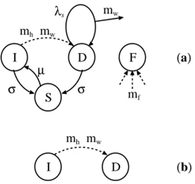
mh I λs mh (a) (b) I D D mw mw mw S F mf µ σ σ
Figure 3: Sensor Agent MAs(a) and Base Station Agent MAb(b) . The
dangling arrows directed to fail state F represent that from any state the reception of mf messages induce a transition to F.
4 states and can perceive 3 types of messages (mh,mf,mw)
but can emit only messages of type mw. MAsis depicted
in Figure 3(a). The meaning of the states is the following:
I - is the idle state: the sensor is quiet until it perceives
a temperature message mhor a warning message mw.
The idle state alternates with the sleeping state S where the sensor is inactive.
D - is the detection state: the node has detected either a
message mhor mwand propagates the warning
mes-sage mwat a rate λsaccording to a given routing
ta-ble.
S - is the sleeping state: the radio device and sensing
equipment are switched off; the wake up transition of rate µ is always to state I.
F - is the fail (absorbing) state and is reached when the
sensor is stricken by the fire front.
The behavior of the MAsagent at the reception of the
mes-sages is the following:
- the reception of mh in state I induces a transition to
state D with probability 1.
- the reception of mf in states I, D or S induces a
- the reception of a warning message mwin state I
ac-tivates the sensor to state D with probability 1 where the warning message mwis replicated with rate λs.
A sensor node can go to sleep (in state S ) either from I or D with rate σ and wakes up at rate µ. When a sensor goes to sleep from state D it forgets any previous incom-ing signal and returns active always in state I.
The base station agent MAb has a simple structure, characterized by an idle state I and a detection state D and is depicted in Figure 3b); MAbis not destroyed by the fire and the transition from I to D occurs at the reception of the temperature message mhor the warning message mw.
In our experiments there is only one base station located in one corner of the grid (Figure 1).
To speed up the alert and save energy, each sensor sends the warning messages to its first neighbor in the direction of the sink according to a predefined routing table whose visual representation is reported in Figure 1c). The flow of messages is indicated by arrows. We define the routing table function RT (v, v′) = 1, when a MAsin position v
is directly connected to a first neighbor MAsin position
v′by an arrow in the routing flow diagram of Figure 1c); RT (v, v′) = 0, otherwise. Given the routing table, the
perception function for the warning message mw is
de-fined as: umw(v, t, i, v ′,t′,j) = 1 if RT (v′,v) = 1 ∧ i = I ∧ j = D 0 otherwise (10)
The interactions between an MAf and an MAsby means of messages mf and between an MAh and an MAs (or
MAb) by means of messages mh are defined according
to the perception functions umf(·) and umh(·) described by
Equations (8).
3.3. Performance indexes
Solving a M3AM means computing the probability
vec-tor πc(t, v) as a function of time t for every MA present
in the area V by means of an equation of type (7). The knowledge of the πc(t, v) provides a complete description
of the model and allows us to compute various perfor-mance measures of interest.
Fire and temperature propagation front - The spatial
propagation of the fire front is given by the spatial prob-ability πBf(t, v) of the agents MAf of being in the burning
state B. Similarly for the propagation of the temperature front.
Mean Fire Propagation Time - The Mean Fire
Propaga-tion Time ηf(v, v′) is the mean time needed by the fire to reach a cell in position v′starting from a cell in position v. ηf(v, v′) is computed by taking the expectation of the ran-dom variable Ω(v, v′) representing the first passage time from v to v′that in turn is computed starting the fire in the
MAf in position v and by making absorbing the MAf in
position v′. To compute ηf(v, v′) we perform the transient
analysis by assuming as initial conditions that the MAfin
position v is in state B (burning) with probability 1 and all the other MAfs are in state I (idle):
πif(0, φ) = 1 if ((φ = v) ∧ i = B) ∨ (φ , v) ∧ i = I)) 0 otherwise
where φ is a generic position that spans over V and i a generic state. Further the burning state B of the MAf in position v′is changed to an absorbing state. From stan-dard probability theory results (see [20]) we have that the Cumulative Distribution Function of Ω(v, v′) is given by:
Pr(Ω(v, v′) ≤ t) = πBf(t, v′)
ηf(v, v′) = E[Ω(v, v′)] = Z +∞
0
(1 − πBf(t, v′)) dt (11)
Mean Message Travel Time - In an similar way, we can
compute the mean travel time ηw(v, v′) needed by a
mes-sage mworiginated from a MAsin position v to reach in
a multi-hop path a MAs in position v′. In particular we investigate ηw(v, vb), the mean travel time taken by a
mes-sage mwto reach the sink. This measure provides an
in-dex of the ”responsiveness” of the WSN in terms of how quickly the network can deliver early warning messages to the sink, before fire arrives.
4. Experiments and Results
All the experiments were performed in the geograph-ical area shown in Figure 1a) with a square grid of L = 50 × 50 cells numbered in the standard Cartesian way. Cell (0, 0) is at the left bottom corner and cell (50, 50) at the right top corner. We locate one MAfand one MAhper
extracted from the RGB coding of the aerial image of the map through an Adobe Flash application as reported in [6]. At time t = 0 all the agents are in their idle state I with probability 1 (πIf(0, v) = πhI(0, v) = 1 ∀v). To start a fire in location φ at t = 0 we assign an initial probability equal to 1 to the burning state B of the MAf in the given location: πBf(0, φ) = 1. The analysis is ccarried out by solving the differential Equations (7) using the TR-BDF2 technique [21]. The computations time ranges from five to ten minutes on a notebook equipped with an Intel Core i5 CPU at 2.5 GHz.x 4 and 5.8GB RAM.
4.1. Fire and Temperature Propagation Front
This Section analyses the dynamic behaviour of the fire and temperature propagation front in an open environment in the presence of obstacles. In the area of Figure 1a) we have located a lake that acts as a barrier preventing the fire to propagate (Figure 4). To model the obstacle, the agents in the cells covered by the lake are removed. The mes-sage emission rates of both MAf and MAh are constant with λf(v) = 0.1 min−1 and λh(v) = 0.2 min−1 ∀v,
re-spectively. The extinguishing rates are the same for both agents in each cell µf(v) = µh(v) but vary from cell to
cell in the range (0 − 0.05) since they are automatically extracted from the map.
We focus on the spatial distribution of the probabil-ity πBf(t, v) of the MAf in the burning state B and of the
probability πh
H(t, v) of the MA
hin the critical temperature
state H. We plot such values in a colored map: darker points in the grid correspond to low probability values, while lighter points indicate higher values. To provide a better visual distinction between the fire and the tem-perature front, we have plotted for the former only prob-ability values in the range 0.7 ≤ πBf(t, v) ≤ 0.9 (cor-responding to yellow color) and for the latter values in the range 0.6 ≤ πhH(t, v) ≤ 0.8 (corresponding to pink color). We study the propagation in two different envi-ronmental conditions: a wind blowing with a constant low speed in a fixed direction from west to east (Figures 4(a-d)) and a wind at high speed with a constant direc-tion from north to south (Figures 4(e-h)). In both condi-tions, the fire originates at position vf = (0, 49), and the
dynamic of the front propagation is plotted at the time in-stants t = 5, 10, 15, 20 min.
Figures 4(a-d) show the propagation with light wind: at minute 5 the initial temperature front in the upper left
corner of the image is just visible; at minute 10 the tem-perature front reaches the lake, and the fire becomes vis-ible in the upper left corner. Proceeding with time, the lake divides the temperature front in two parts and the fire grows covering a larger zone as clearly visible at minute 15. Finally at minute 20, the temperature front exits from the map and the fire propagation is hindered by the lake.
With a strong wind the propagation is significantly quicker and with a different dynamic as shown in Figures 4(e-h). At minute 5 the temperature front reaches the west side and surpasses the east side of the lake, while the fire is still in the corner. At minute 10 the fire reaches the lake and the temperature front is already beyond the map. Also in this case the fire is hindered by the lake, but the wind is strong enough to let the fire circumvent the lake as shown at minute 15. From now on the fire is free to spread beyond the lake and to cover a significant part of the whole area (minute 20). Finally, we have supposed that there is a critical structure (a house, a village) in the left lower corner of the map at the cell vcrit = (0, 0) and
we have measured the mean time ηf(vf,vcrit) needed by
the fire to reach the critical location. With a light wind ηf(vf,vcrit) is about 39 min, whereas with a strong south
directed wind it is reduced to about 17 min.
4.2. WSN analysis
This Section is dedicated to analyse the WSN in isola-tion, i.e. without considering its interaction with the tem-perature and fire agents. This analysis is intended to be useful in a preliminary design phase to tune the structure and the parameters of the WSN. The parameters that in-fluence the performance of the WSN are, primarily, the distance w (measured in number of cells), the sending rate of warning messages λsand the duration of the sleeping
cycle α of active-sleeping periods determined by the val-ues of the rates σ and µ:
α =100 σ
σ + µ (12)
The experiments have been performed considering the ge-ographical area of Figure 1b) in which the MAs sensor
agents are located at the intersection of the dashed grid with step w and one single sink agent MAbis always
lo-cated in a fixed position vb = (48, 48). The analysis is
concentrated to find the average travel time of the warn-ing message ηw(v
0 0.2 0.4 0.6 0.8 1 (a) t=5 min. 0 0.2 0.4 0.6 0.8 1 (b) t=10 min. 0 0.2 0.4 0.6 0.8 1 (c) t=15 min. 0 0.2 0.4 0.6 0.8 1 (d) t=20 min. 0 0.2 0.4 0.6 0.8 1 (e) t=5 min. 0 0.2 0.4 0.6 0.8 1 (f) t=10 min. 0 0.2 0.4 0.6 0.8 1 (g) t=15 min. 0 0.2 0.4 0.6 0.8 1 (h) t=20 min. Figure 4: Fire and temperature propagation front in the presence of an obstacle
vb, as a function of the position va, of the sleeping cycle
αand of the distance w. To generate the warning signal, at time t = 0 the single sensor in position vais made
ac-tive in the detection state D by setting πs
D(0, va) = 1, and
remains active so that for the duration of the entire exper-iment it emits warning messages mw at rate λs. All the
others MAsagents follow the same sleeping-active cycles
with sleeping cycle α and are assigned an initial probabil-ity πs
I(0, v) = 1 − α and π s
S(0, v) = α for all v , va.
In the experiments we have considered a set of posi-tions va = {(0, 0), (24, 24), (36, 36)}, two values of the
sending rate λs ={1.667, 0.2} sec−1 (corresponding to a
mean time between message emissions of 0.6 and 5 sec, respectively) and two sizes of the grid topology with (w = 6) and (w = 12) (to change the number of hops to reach the sink). Further, the sleeping cycle α varies in the range [0 − 95]. The results are shown in Figure 5. In all the experiments two effects are always visible. First, the travel time of the warning messages ηw(v
a,vb) is
di-rectly proportional to the distance between the location va
generating the message and the sink vb; second, an
incre-ment of the sleeping percentage increases the travel time since it increases the probability that at each hop a sensor wastes time sending messages to a sleeping sensor.
How-ever, such an increment depends on the network charac-teristics. With a high transmission rate (λs= 1.667 sec−1)
this effect becomes significant only for very high sleeping percentages (of the order of α = 90%) as shown in Figure 5(a-b). A stronger effect appears with a lower transmis-sion rate of λs = 0.2 sec−1 as shown in Figure 5(c-d)
where a significant increment in the mean travel time ap-pears for lower values of α particularly in the case w = 6.
4.3. WSN detecting incoming fire
In this Section we combine the fire and temperature propagation model of Section 3.1 with the WSN detec-tion and warning model of Secdetec-tion 3.2. The model lo-cates one MAf and one MAh in each cell, and one MAs every w = 8 cells. The fire propagation rate λf and the
temperature propagation rate λhare constant over all the
cells with λf = 2.0 min−1 and λh = 4.0 min−1,
respec-tively. For each cell the wind intensity is low and the di-rection constant. To show that the model can handle non-homogeneous and location-dependent phenomena [7], the extinction rate of both fire and temperature are automati-cally extracted from the colored map in Figure 1(a) so that any cell may have a different rate value. In the present set of experiments those values range from 0.2 to 0.9 min−1.
0 5 10 15 20 25 30 35 40 45 50 55 60 65 70 75 80 85 90 95 100 0 10 20 30 40 50 60 70 80 90 η w( va , vb ) [sec] α va=(0,0) va=(24,24) va=(36,36) (a) λs= 1.667 sec−1w = 12. 0 5 10 15 20 25 30 35 40 45 50 55 60 65 70 75 80 85 90 95 100 0 10 20 30 40 50 60 70 80 90 η w( va , vb ) [sec] α va=(0,0) va=(24,24) va=(36,36) (b) λs= 1.667 sec−1w = 6. 0 5 10 15 20 25 30 35 40 45 50 55 60 65 70 75 80 85 90 95 100 0 10 20 30 40 50 60 70 80 90 η w( va , vb ) [sec] α va=(0,0) va=(24,24) va=(36,36) (c) λs= 0.2 sec−1w = 12. 0 5 10 15 20 25 30 35 40 45 50 55 60 65 70 75 80 85 90 95 100 0 10 20 30 40 50 60 70 80 90 η w( va , vb ) [sec] α va=(0,0) va=(24,24) va=(36,36) (d) λs= 0.2 sec−1w = 6.
Figure 5: Travel time of warning messages varying the sleeping time percentage and for different always active sensor positions.
The fire starts in the left lower corner in position vf =
(0, 0), while the sink is located at the opposite corner in position vb = (48, 48). Each sensor is tuned with a low
sleeping percentage α = 20%. The sending rate of the warning messages is λs= 100 min−1, about two orders of
magnitude greater than the rate of the fire propagation. In the figures the sensors are spotted as small squares.
Figures 6(a-d) show the spatial and time evolution of the probabilities of having MAf in the burning state B,
MAh in the critical temperature state H and MAs,bin the detection state D. The figures capture the dynamics of the model at the time instants t = 2, 5, 20, 30 min. As in previous experiments, to distinguish the fire and the temperature front, all the values of 0 ≤ πBf(t, v) ≤ 1.0 are plotted whereas for the temperature only the values 0.4 ≤ πh
H(t, v) ≤ 0.8 are plotted in purple/blue (dark)
color. For the sensors, all the values of 0 ≤ πs
D(t, v) ≤ 1.0
are drawn on the figures. To improve the visibility of the sensors dynamics, Figures 6(e-h) isolate the spatial
prob-ability πs
D(t, v) for the sensors MA
s,b, only, and with a
dif-ferent color scale (from white/yellow for low probabilities to dark blue for high probabilities).
The fire spreads slowly in an approximately circular way with slight variations due to the non-homogeneous extinction rates and the light wind. Due to the high cov-erage of monitored area, the WSN can detect the fire al-most immediately: even at t = 2 min, when the fire is just started at the lower-left corner, the path of colored squares along the diagonal of the area indicates a flow of warning messages towards the sink. At t = 5 min the probability that such sensors have detected the fire is almost one. At
t = 20 min, other sensor routes, leading from the fire to
sink, starts to appear: this can be used by the base station to monitor the extension of the fire. At t = 30 min, al-most all the sensors have detected the fire, that has already reached half-way to the sink. From the sensor messages, the base station can estimate the speed and extension of the fire front, and properly direct the actions of the
0 0.2 0.4 0.6 0.8 1 S (a) t=2min. 0 0.2 0.4 0.6 0.8 1 S (b) t=5min. 0 0.2 0.4 0.6 0.8 1 S (c) t=20min. 0 0.2 0.4 0.6 0.8 1 S (d) t=30min. 0 0.2 0.4 0.6 0.8 1 S (e) t=2min. 0 0.2 0.4 0.6 0.8 1 S (f) t=5min. 0 0.2 0.4 0.6 0.8 1 S (g) t=20min. 0 0.2 0.4 0.6 0.8 1 S (h) t=30min. Figure 6: The WSN detects the incoming fire and alerts the base station.
fighters.
5. Discussion 5.1. Complexity
The state space of the example discussed in Section 4 has the following size. There are ℓ2= 2500 MAf (with 3
states) and MAh (with 2 states ). There are (ℓ/w)2 = 64 MAs(with 4 states) and there is one MAb(with 2 states). The total number of states of the model is therefore:
NT = 32500× 22500× 464× 2 (13)
which is a number that is hardly explored even by simu-lation. Our analytical technique is feasible since we solve separately 2500 Equations of the form (7) for MAf, 2500 for MAh, 64 for MAs and 1 for MAb. An exponential
complexity is reduced to a linear complexity. However, to arrive to solve one Chapman-Kolmogorov equation of type (7) for a given agent of class c, we need to com-pute first the influence matrix Kc(t, v). If we denote by
n∗= Max{nc} the largest dimension of the state space of
MA of any class, the computation of matrix Kc(t, v)
re-quires M computations of the diagonal matrixΓc(t, v, m),
one for each message type. MatrixΓc(t, v, m) has at most
n∗entries that account for all the interactions with all the
MAs in the whole area V during sojourn in state i, (see Equation (5)). Let NI be the number of such possible
in-teractions; in the worst-case each MA interacts with all the other ones and hence NI = C n∗ℓ2. In the
worst-case the complexity of the computation of matrix Kc(t, v) is O(n∗NI) = O(C n2∗ℓ2). In the described scenario the
worst-case complexity would be O(4 × 42 × 2500) = O(160000).
However, and this is the main point of the technique, the worst-case complexity is greatly reduced since the in-teraction of each MA is often limited to a subset of mes-sage types and is confined to a restricted region around the position of the MA by means of the perception function
u(·). In our scenario each MAfperceives messages only of type mf from MAfs that are inside the propagation ellipse
(as described by the perception function in (8)) that cov-ers on the average 24 cells. MAhperceives messages only
of type mh from MAfs or MAhs that are inside the same
propagation ellipse. Each MAs perceives messages of
types mf, mhand mwfrom MAfs or MAhs or MAs
accord-ing to the routaccord-ing table indicated with arrows in Figure 1. As can be inferred from Figure 1 each MAsperceives
Fi-nally, the sink MAbperceives messages of types m
hand
mwfrom the 3 first neighboring locations only (Figure 1).
For such reasons, in our scenario the real number of in-teractions to be taken into account in the computation of matrix Kc(t, v) is approximately NI∗≤ 200, with an
enor-mous reduction in comparison with the worst-case. The Equations (7) are solved by resorting to numerical iterative techniques over a discretized time interval. The 0 − TW mission time is uniformly discretized with step
∆t yielding T∆ = TW/∆t time points. Thus, in the
worst-case the time complexity of the solution algorithm turns out to be O(T∆Mℓ4C2n2∗). In our scenario the complexity
is reduced to O(NI∗T∆ℓ
2C Mn
∗) since, as outlined earlier,
the possible interactions of each MA with its neighbors are limited (that is, NI∗ << NI = ℓ
2Cn
∗). The capability
of the M3AM to confine and localize the interactions is
one of its main peculiar properties that is exploited in any practical application.
5.2. Environmental protection systems
Environmental protection systems are usually imple-mented with a network of Intelligent Guards against Dis-asters(iGaDs) devices [3] which locally maintain location information and behave according to their own position. Such feature can be naturally included in MAM models. For instance, the perception function can be used to model power decay of a message transmission depending on the relative distance between source and destination. More-over, the work in [16] shows that MAM can also repre-sent and evaluate distributed gradient-based routing algo-rithms for WSN with time-varying topology.
The ability of iGaDs network to deliver early warning depends on network parameters, such as the frequency of forwarding, the transmission range and the network topol-ogy. But it is also affected by the physical characteristics of the considered environmental threat, such as its prop-agation speed and its direction. Thus, a proper model should take into account both the monitoring system and the disaster dynamic to capture their interdependencies. To the best of our knowledge, such holistic approach is rarely applied. On the one hand, iGaDs are evaluated by analytic or simulative models in which the disaster event is represented by just a probability of occurrence or a rate; on the other hand, disaster dynamics are evaluated by sim-ulation of complex model without considering the iGaDs. Instead, in this work we have shown that a unified MAM
model, even with the simplified fire propagation model in Section 3.1, can provide useful insight about the iGaDs system performance.
6. Conclusions
In this work we presented a modeling technique to study, within a single unified framework, the propaga-tion of an environmental hazard (a forest fire) together with the performance of a WSNs deployed to timely de-tect the hazard by sending warning messages to a base station. Despite the huge complexity of the state space of the overall model, the MAM formalism has been able to build up a set of analytical equations that are numeri-cally tractable. The main feature of the MAM models is its ability to confine the interaction of each entity of the distributed system to a delimited environment as it is of-ten observed in many real large-scale distributed applica-tions. Further, the MAM model is sensitive to the position of each entity and to their relative distances so that highly non-homogeneous phenomena can be naturally captured. Along the line presented in this paper, the methodology can be refined to improve the WSN alarm protocols, to optimize the sensor placement, and to optimize the model parameters, to increase the sensor lifetime and reduce the time to detect the hazard.
However, various new directions can be envisaged to expand and improve the MAM modeling technique. In-vestigate more abstract interaction mechanisms not based on the message passing paradigm combined with a per-ception function. Include the mobility of the entities. De-fine a high level language to facilitate the description of the model.
References
[1] J. Yick, B. Mukherjee, D. Ghosal, Wireless sensor network survey, Computer Networks 52 (12) (2008) 2292 – 2330.
[2] P. Corke, T. Wark, R. Jurdak, W. Hu, P. Valencia, D. Moore, Environmental wireless sensor networks, Proceedings of the IEEE 98 (11) (2010) 1903–1917. URLhttp://eprints.qut.edu.au/42703/
[3] J. W. Liu, C.-S. Shih, E. T.-H. Chu, Cyberphysical elements of disaster-prepared smart environments, Computer 46 (2) (2013) 69–75.
[4] B. Son, Y. He, J. Kim, A design and implementation of forest-fires surveillance system based on wireless sensor networks for south Korea mountains, Inter-national Journal of Computer Science and Network Security 6 (9B) (2006) 124–130.
[5] J. Lloret, D. B. M.l Garcia and, S. Sendra, A wireless sensor network deployment for rural and forest fire detection and verification, Sensors 9 (2009) 8722– 8747.
[6] D. Cerotti, M. Gribaudo, A. Bobbio, C. Calafate, P.Manzoni, A Markovian agent model for fire prop-agation in outdoor environments, in: Computer Performance Engineering (EPEW2010), Springer -LNCS, Vol 6342, 2010, pp. 131–146.
[7] A. B. D. Cerotti, M. Gribaudo, Disaster prop-agation in inhomogeneous media via markovian agents, in: Critical Information Infrastructure Secu-rity, Springer Verlag - LNCS, Vol 5508, 2009, pp. 328–335.
[8] M. Bahrepour, N. Meratnia, M. Poel, Z. Taghikhaki, P. Havinga, Distributed event detection in wireless sensor networks for disaster management, in: 2nd International Conference on Intelligent Networking and Collaborative Systems (INCOS), 2010, IEEE, 2010, pp. 507–512.
[9] Y. Ma, M. Richard, M. Ghanem, Y. Guo, J. Hassard, Air pollution monitoring and mining based on sen-sor grid in London, Sensen-sors 8 (6) (2008) 3601–3623. [10] K. Khedo, R. Perseedoss, A. Mungur, A wireless sensor network air pollution monitoring system, In-ternational Journal of Wireless & Mobile Networks 2 (2) (2010) 31,45.
[11] M. Suzuki, S. Saruwatar, N. Kurata, H. Morikawa, A high-density earthquake monitoring system using wireless sensor networks, in: Proceedings of the 5th international conference on Embedded networked sensor systems, SenSys ’07, ACM, New York, NY, USA, 2007, pp. 373–374.
[12] G. Werner-Allen, K. Lorincz, M. Rui, O. Marcillo, J. Johnson, J. Lees, M. Welsh, Deploying a wireless sensor network on an active volcano, IEEE Internet Computing 10 (2) (2006) 18–25.
[13] F. Yu, A survey of wireless sensor network simula-tion tools, http://www1.cse.wustl.edu/ jain/cse567-11/ftp/sensor/index.html (2011) 1–10.
[14] M. Gribaudo, D. Cerotti, A. Bobbio, Analysis of on-off policies in sensor networks using interact-ing Markovian agents, in: 4-th Int Work Sensor Networks and Systems for Pervasive Computing -PerSens 2008, 2008, pp. 300–305.
[15] M. C. Guenther, J. T. Bradley, Higher moment anal-ysis of a spatial stochastic process algebra, in: Com-puter Performance Engineering, Springer - LNCS, Vol 6977, Springer, 2011, pp. 87–101.
[16] D. Bruneo, M. Scarpa, A. Bobbio, D. Cerotti, M. Gribaudo, Markovian agent modeling swarm in-telligence algorithms in wireless sensor networks, Performance Evaluation 69 (2012) 135–149. [17] M. Gribaudo, D. Manini, C.-F. Chiasserini,
Study-ing mobile internet technologies with agent based mean-field models., in: A. N. Dudin, K. D. Turck (Eds.), ASMTA, Vol. 7984 of Lecture Notes in Com-puter Science, Springer, 2013, pp. 112–126. [18] D. Cerotti, M. Gribaudo, A. Bobbio, D. Bruneo,
M. Scarpa, An intelligent swarm of markovian agents, Tech. rep., Politecnico di Milano, Italy, TO APPEAR.
[19] M. Dorigo, T. St¨utzle, Ant Colony Optimization, MIT Press, 2004.
[20] K. S. Trivedi, Probability and statistics with reliabil-ity, queuing and computer science applications, John Wiley and Sons Ltd., Chichester, UK, 2002. [21] R. E. Bank, W. M. C. Jr., W. Fichtner, E. Grosse,
D. J. Rose, R. K. Smith, Transient simulation of sil-icon devices and circuits, IEEE Trans. on CAD of Integrated Circuits and Systems 4 (4) (1985) 436– 451.