UNIVERSITA’ DEGLI STUDI DI MESSINA
XXIX CICLO DOTTORATO DI RICERCA IN FISICA
EFFECTS OF INSTRUMENTAL ENERGY
RESOLUTION ON THE MEASURED MSD AS
OBTAINED BY ELASTIC INCOHERENT
NEUTRON SCATTERING DATA
Thesis of:
Dr. Salvina Coppolino
Tutor: Chiar.mo Prof. Salvatore Magazù
PhD Coordinator: Chiar.mo Prof. Lorenzo Torrisi
Table of contents
Introduction ………..…..……….. I
Motivation………...…... II
Thesis outline………..………...……
Chapter 1 Characterization of molecular motions in condensed matter systems using complementary techniques………..…
1
1.1 General Introduction to Molecular Dynamics and spectroscopic
techniques……….. 1
1.2 Models for translational and rotational diffusive motions and for vibration motions……….. 2
1.3 The principle of a spectroscopic experiment: Definitions………... 3
1.3.1 First step: Probe-system coupling……….. 4
1.3.2 Second step: Calculation of Wnm………... 5
1.4 Neutron Scattering ……… 8
1.4.1 Properties of the neutron probe………. 8
1.4.2 Nature of the neutron-nucleus interaction……… 10
1.4.3 Coherent and incoherent scattering contributions and relative cross-sections……… 11
1.4.4 Neutron scattering experiment………... 13
1.4.5 Scattering from incoherent scatterers……… 16
1.4.6 Incoherent “Quasi-elastic” Spectra……… 19
1.4.6.1 Rotation and diffusion spectral contributions……….. 19
1.4.6.2 Translational diffusion spectral contribution……….. 20
1.4.6.3 Superposition of rotational and translational spectral contributions……….. 23
1.4.6.4 Vibrational spectral contribution……….. 23
1.4.7 The Elastic Incoherent Structure Factor (EISF)………... 23
1.5 Absorption and Scattering of Electromagnetic Waves: Dielectric and Infrared Absorption, Raman and Rayleigh Scattering………. 26
1.5.1 Electromagnetic Waves and photons……… 26
1.5.2 Long Wavelength e.m. waves- matter interaction………... 28
1.5.3 Dielectric and infrared absorption: interaction with permanent dipoles: Introductive definitions………... 29
1.5.3.1 Dielectric absorption: permanent dipoles………. 33
1.5.3.2 Infrared (IR) absorption: derivative dipoles………... 35
1.6 Interaction with induced dipoles: absorption and scattering of photons………... 40 1.6.1 Introductive definitions………. 40
1.6.2 Rayleigh and Raman scattering of light……….. 42
1.6.3 Raman scattering of light: derivative polarizability tensor……….. 44
1.6.4 Rayleigh scattering of light: permanent polarizability tensor…….. 49
Chapter 2 Recent Development on Elastic Incoherent Neutron Scattering (EINS) and Resolution Elastic Neutron Scattering (RENS)……….… 54
2.1 Introduction……… 54
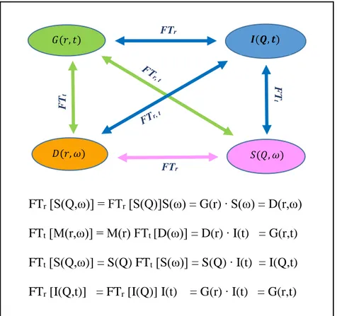
2.2 Fourier Transform (FT)……… 55
2.3 Definition and relations existing between the functions G(r ⃗,t), I(Q ⃗,t), S(Q ⃗,ω) and D(r ⃗,ω)………...……….. 57
2.4 Theoretical approach on elastic neutron scattering (EINS)………... 60
2.5 RENS…….………... 67
Chapter 3 Mean Square Displacement (MSD)……….… 71
3.1 Brownian motion……….….. 71
3.2 Definition……… 73
3.3 Self-Distribution Function Procedure……….. 74
3.4 MSD in translational motions……… 77
Chapter 4 Investigated systems and methods………... 81
4.1.1 Primary Structure of Proteins……… 84
4.1.2 Secondary Structure………. 84
4.1.3 Tertiary Structure………. 85
4.2.4 Quaternary Structure………... 86
4.2 Lysozyme………...………... 87
4.3 Characteristic of the used spectrometers………. 91
4.3.1 IN10………... 91
4.3.2 IN13………... 95
Chapter 5 Result and discussion………. 97
5.1 Theoretical results……….. 97
5.1.1 Gaussian Approximation for MSD evaluation………. 97
5.1.2 Data Normalization criteria………... 98
5.1.2.1 Normalization performed on the Gaussian function…... 98
5.1.2.1.1 Normalization by multiplication………. 98
5.1.2.1.2 Normalization by sum……….. 99
5.1.2.1.3 Normalization considering two different temperatures……… 100 5.1.2.2 Normalization performed on the logarithm of the Gaussian function……… 102 5.1.2.2.1 Normalization by multiplication………... 102
5.1.2.2.2 Normalization by the sum of the logarithm…... 103
5.1.2.2.3 Normalization by the sum of logarithm argument……… 105
5.2 Experimental results and comparison with developed theory……… 105
5.2.1 Characteristics of IN10 and IN13 spectrometers for lysozyme experiments………... 105
5.2.2 Data obtained through the spectrometers IN10 and IN13 on the analyzed samples……… 107
5.2.3 Comparison between the MSD data obtained in experiments conducted on lysozyme with IN10 and IN13 spectrometers…………. 113
Conclusions……… 130
Aknowledgements………. 132
Introduction
The introductory chapter presents the work motivation and concludes with a brief description of the thesis.
Motivation
The main focus of the present thesis is Elastic Incoherent Neutron Scattering (EINS) experimental data collected for dry and hydrated (H2O and D2O) lysozyme samples; this study was performed as a
function of the exchanged wave vector.
Later, the analysis of mean square displacement on the collected elastically scattered intensity data as a function of the exchanged wavevector has been performed.
What has been done to make a comparison between the values of mean square displacement obtained with different instruments.
In particular the data analyzed were obtained at the Institute Laue Langevin (Grenoble, France) by using two spectrometers, IN13 and IN10 working at the energy resolution value of 8 μeV, corresponding to an elastic time resolution of 516 ps, and at the energy resolution value of 1 μeV, corresponding to an elastic time resolution of 4136 ps.
Since the experimentally obtained neutron scattering data depend on the employed spectrometer instrumental characteristics, the system observables as mean square displacement (MSD), are influenced by instrumental effects.
Then, there is the problem of comparing data from spectrometers with different instrumental resolutions.
In order to do this, we faced the problem of normalization of data, which allow to solve it comparing the MSD system.
There are many ways in which we can address the problem of normalization but, after careful analysis, we deduced that only a few of them do not change the value of the MSD.
The comparison, in particular, is performed at very low temperatures (T < 80 K). In such a case occur only vibrational motions and the MSD system can be considered almost constant <r 2> (t) → <r 2>(V).
Thesis outline
The current thesis is organized as follows:
Chapter 1, Complementary approaches for the characterization of molecular motions in condensed matter systems. This chapter deals with the use of complementary spectroscopic techniques and numerical techniques for the study of systems of biophysical interest. In particular, the focus is addressed on laser light scattering, infrared absorption, neutron scattering for the characterization of the space-time correlations of physical systems.
Chapter 2, Recent Development on Elastic Incoherent Neutron Scattering and Resolution Elastic Neutron Scattering (RENS). It deals with the collection of elastic neutron scattering intensity both as a function of temperature (EINS) and resolution (RENS).
Chapter 3, Mean Square Displacement (MSD). After an introduction on the Brownian motion,
it describes the concept of MSD and the SDF procedure: a recipe for the MSD evaluation from EINS experiments.
Chapter 4, Investigated systems and methods. A description of the investigated systems is reported. More specifically, these are dry and hydrated (H2O and D2O) lysozyme samples.In
addition, the description of the protein structure and of IN10 and IN13 spectrometers is given.
Chapter 5, Results and discussion. It shows the different normalization procedures applicable to data obtained experimentally in laboratory, so that they can be compared. In particular, it focuses on those useful for normalization of MSD.The resultsobtained from applied approaches with different normalizzation procedures and the obtained values of MSD for dry and hydrated (H2O and D2O) lysozyme are reported.
Chapter 1
Characterization of molecular motions in condensed matter
systems using complementary techniques
1.1 General introduction to molecular dynamics and spectroscopic
techniques
The spectroscopy experiments and molecular dynamics calculations allow us to approach the study of molecular motions in liquids in two complementary ways [1].
By means of spectroscopic techniques, it is possible to use a probe as electromagnetic waves (e.m.), centrifugal, neutrons, ..., prepared in a known state, that interacts with the degrees of freedom of the investigated system. The probe state changes are due to the interaction, (for example the e.m. wave is dispersed) and such a change reflects the dynamic properties of the system. The result appears normally in the form of a spectrum of energy that must be interpreted in terms of molecular motions. As will be seen below, each spectrum is proportional to the time Fourier transform of a well-defined correlation function (c.f). A c.f is the average balance of the set of two molecular dynamics variables product taken at time 0 and the time t. A means now widely used to extract the physical information from a spectrum is to use the concept of a dynamic model. This model is characterized by one or more equations that govern the rates of evolution of molecular dynamics variables. These equations allow to calculate the correlation functions and, after Fourier transforming, the theoretical spectrum. The parameters of the model may be deducted (jump time, gyration radius...) and the experimental spectrum are compared with the spectrum obtained
If, however, we face the problem by molecular dynamics, we examine about N = 1000 rigid molecules, we consider the potential intermolecular coupling, and we choose the boundary and initial conditions (i.e. the volume and energy) and numerically solve the coupled equations 6N of motion. Based on these results it can generally calculate a physical quantity associated with the system (balance amount as well as time dependent). But the method is limited by computer memory and time; this method can not be very good to test long-standing and long-range phenomena, as described, for example, from hydrodynamic theory theory and critical phenomena. This in particular because:
N is always small compared to the number of particles in a real sample (the volume of sample tested is always very small) ;
the number of integration steps is necessarily finished then the time scale is relatively small.
The restriction to pair potentials and to classical mechanics is the other limitation of this method. Consequently a quantum description is therefore necessary as important phenomena such as vibration can not be included. The main interest of the molecular dynamics method is to give typical results that can be compared to results obtained from experiments on real liquids.
1.2 Models for translational and rotational diffusive motions and for
vibration motions
To describe molecular translation, rotation and vibration [1] a large number of models have been developed and the main ones are listed below:
1. Translation
- Langevin model describes the molecular centre of mass. Then the particle is assumed to be submitted to two forces: a viscous force and a random force. In the limits of very weak and very strong viscosity, one finds the free
translation and the uniform translational diffusion, respectively. In the
latter case, the motion is characterized by a single diffusion coefficient Dt
(isotropic medium). On the other hand, collective translational motions are usually described in terms of longitudinal acoustic waves and thermal diffusivity in a hydrodynamic theory.
2. Rotation
- In this case many models have been devised and can be summarized in two major groups inertial and stochastic models.
The inertial models are plausible in low density compounds from spheroidal molecules systems infact the molecules are essentially rotating, but undergo random collisions that modify their dynamic state. Examples of inertial models are: the free rotation model (collisions) and diffusion models extended (so-called J and Gordon M models) where, during the collision, the orientation of molecules do not change but their angular
momentum J is randomized.
- The stochastic models are plausible in highly condensed systems. In this case the molecules are essentially non rotating, the motions occurring by rapid rotational jumps over barriers. An example is the Debye model (isotropic diffusion characterized by a single diffusion coefficient Dr) so the anisotropic diffusion model and the model of Ivanov (jumps of isotropic finite angle).The distinction between inertial and stochastic models is not clear, especially when the time between jumps or collisions is of the order of (kBT / I) 1/2, the average time to jump to thermal motion rotation. In this case, the model should combine both aspects as is the case for example, in the Langevin model for the rotation. Other models in which they are combined translation and rotation have been imagined. For example, remember the violent collision model in which molecules move freely, except during collisions that instant randomize both the position and the angular momentum. As for the collective rotational motions, some recent experiments of diffusion of light seem to require a description in terms of coupling between shear waves and molecular rotations.
3. Vibrations
Regarding the molecular vibrations, little is known so far. However, it appears that a large number of mechanism may be the cause for the vibrational relaxation, in particular coupling with all the other degrees of freedom: rotation, translation and other vibrations.
Obviously this does not exhaust the study of the subject which is much more extensive than we treated
1.3 The principle of a spectroscopic experiment: definitions
Given a system (i.e. a molecular liquid) which we call reservoir R, formed by N particles, in thermal equilibrium T. This reservoir is characterized by its Hamiltonian HR whose
eigenvalues and eigenstates are Em’ and respectively [1].
We wonder how the molecular properties of this system vary with time. For this reason, we consider another system (e.g. the e.m. field, the neutron field, a spin system) which
'
we call the probe P. It is characterized by its Hamiltonian HP whose eigenvalues and
eigenstates are labelled Em and .
The probe has the ability to join with the dynamical variables of the reservoir and this coupling is characterized by an Hamiltonian HC.
1.3.1 First step: Probe-system coupling
Initially, we consider the probe in a defined dynamical state (e.g. e.m. waves or neutrons are collimated and monochromatized). Being at thermal equilibrium, the reservoir R can be in any state with the probability
p
m, given by the Boltzmann law: ) exp( 1 ' ' m R m E Z p
(1.1) with
' ') exp( m m R E Z (1.2) and T kB 1 (1.3)Where
k
Bis the Boltzmann constant.The figure below shows a sketch of a spectroscopic experiment.
Figure 1.1 Sketch of a spectroscopic experiment
Because of the interaction hc turned on, the state of the probe P can change with time from the inistial state to a final state . If HC is small compared to HP and HR,
in the linear approximation this change can be characterized by a probability per unit time
m m ' m m n
RESERVOIR
R
PROBE
P
Interaction Hamiltonian Hc
nm
W
. The purpose of any spectroscopic experiment is to measure a quantity which isproportional to
W
nmas a function of n or . This becauseW
nm measurement yieldsinformation about what is happening in R (e.g. the molecular motions) being that
W
nm isa function of operators of R. Then what we need to do is to calculate
W
nmand relating it to a measurable quantity.1.3.2 Second step: Calculation of W
nmThe calculation of
W
nm goes made considering the total system formed by the probe plusthe reservoir. The corresponding eigenstates are symbolized by m . In the linear approximation, we have:
' ' ' ' ' m n m nn mm nm W p W
(1.4)where Wn’nm’m is the probability for unit time that this total system changes from the state
m to the state n n' due to HC and its value is given by the following Fermi rule .
m m n n
C nn mm n n H m m E E E E W ' ' 2 ' ' 2 ' ' (1.5)The delta function that we see is obtainable by the energy conservation principle. Defining HC as the average of HC between the initial and final state of the probe:
C
H n Hint m (1.6) Defined in this way, HC is an operator that acts on the states of the reservoir only.
With the following definitions:
E
m
E
n (1.7) ' ' m nE
E
(1.8)considering the equation written above, the probability
W
nm is written: ) ( ' ' ) exp( 2 ' ' 2 ' ' ' 2 C nm n m R m nm n H m Z E W (1.9) m ' m ' mThis expression is suitable to describe discrete peaks in a spectrum, as is the case for a purely quantum system, thanks to the presence of the δ function [1].
Using the fact that HC is an hermitian operator and by using the integral expression for
the δ function is possible using another equivalent expression for
W
nm for describing more complicated system. We have: 2 ' 'H m n C n'HC m' m'HC n' (1.10a) and
i t m n m n dte( ) ' ' ' ' 2 1 (1.10b)inserting eqs. (1.10a) and (1.10b) in eq.(1.9) and using Eq. (1.8), we obtain
t i t E i C t E i C m n R E nm m H n n e H e m e Z e dt W m n m
1 ' ' ' ' ' ' ' ' 2 (1.11)The double sum is simply the expression of a trace in the R Hilbert space. We thus have:
i t C C R nm dtTr H H t e W
12 (0) () (1.12)where
R is the density matrix of R at thermal equilibrium:
R
R H H R e Tr e (1.13)and HC(t)is the Heisenberg representation of operator HC:
t E i C t E i C m n e H e t H ' ) ( (1.14) The quantity
) ( ) 0 ( H t H Tr C C C C CH R H
HC (0)HC(t) (1.15)If the reservoir is classical, then HC is a classical function of the variables of R
and C
tC CH
H should be replaced by its classical equivalent. Defining the spectral density
C CHH
C as the time Fourier transform of C (t)
C CH H :
C t e dt C i t H H H HC C C C ( ) 2 1 ) ( (1.16)and using eq.(1.12), the probability of transition
W
nmis finally written:
C CH H nm C W 22 (1.17)An important point is to relate the probabilities for the direct transition
W
nm and theinverse transition
W
mn is finally. Changing
into
in the above equations, after a little algebra, we obtain:nm
mn e W
W (1.18)
This is the Kubo-Ayant theorem which means that, in the linear approximation, the probability per unit time for the transition from one level to another is proportional to the population of this level.
In summary, to describe any spectroscopic experiment, we are led to define the reservoir, the probe, the interaction HC and calculate the average value HC, its
correlation function C (t)
C CH
H and the probability
W
nm. To be complete, we must relatenm
W
to a measurable quantity. However, this relationship is clearly dependent on the typeand details of the experiment (e.g. an absorption experiment, a scattering experiment, a relaxation experiment) and no general formula can be given. We shall thus establish it for each particular case treated below.
1.4 Neutron Scattering
In this part we will talk about neutron, describing how they can be used to study molecular motions. We begin first remembering the properties and associated concepts, then describe the principles of a neutron scattering experiment, deduce the relevant correlation function, relate it to the scattered intensity and give some illustrative examples [1].
1.4.1 Properties of the neutron probe
The free neutron [1] is an elementary particle with zero charge and spin ½, liberated for example during the process of fission of a heavy nucleus. In a nuclear reactor, the neutrons are thermalized by the atoms of the moderator, yielding a Maxwellian distribution of velocities v peaked at some v such that the average (kinetic) energy Eis
T k v m E n B 2 3 2 1 2 (1.19)
where m is the mass of the neutron. n
Neutrons can also be considered as plane waves of wave number k or wavelength
k
2 . The relationships between particle and wave aspects are:
n m k E 2 2 2 (1.20) and n m k v (1.21)
For thermal neutrons (T=300K), we have E=26 meV and =1.8 Å. It is important to note that these values have the same order of magnitude as the intermolecular energies and molecular dimensions, respectively. In fig. 1.2 the spatial scales interested by neutron probe are reported.
Fig. 1.2: Spatial scales interested by the neutron probe.
Finally, considered as quantum objects, neutrons are characterized by wave functions
k
such thatk
=e
ikrV
1
(1.22)where V is the “volume of quantization” to be identified with the volume of the irradiated sample. In this volume, the density of states of momentum k is given by
3
)
2
(
)
(
k
V
(1.23)Using the expression below of the volume element in spherical coordinates:
k dkd k d 2 (1.24) with:
d = the solid angle corresponding to dk around k
we deduce that the number of independent neutron states between k and k+dk is:
V
k
d
k
d
k
d
k
3 2
)
2
(
)
(
(1.25)
Fig. 1.3: “Identity card” of neutron
1.4.2 Nature of the neutron-nucleus interaction
A neutron interacts with a nucleus through nuclear and magnetic forces. Concerning the nuclear part, since nuclear interactions are very short range compared to the (thermal) neutron wavelength, it can be shown that the interaction potential between a neutron located at rand a nucleus located at ri can be written as
) ( 2 ) ( 2 i i n r r b m r V (1.26)
In the expression we have written now (the so-called Fermi pseudo-potential), the scattering length bi characterizes the interaction and is independent of neutron energy. bi
can be positive or negative depending on the attractive or repulsive nature of the interaction. Is so difficult theoretically calculate the value of bi and for this reason it is
calculated experimentally
For the magnetic interaction, the neutron interacts with the spins through the dipole-dipole coupling. Compared to the nuclear interaction, for diamagnetic systems it is always insignificant and shall not be considered in the following. fig. 1.4 shows the Maxwell neutron velocity distribution.
Fig. 1.4: Neutron velocity distribution
1.4.3 Coherent and incoherent scattering contributions and relative
cross -sections
Consider a set of a given atomic species, i, in which many isotopes possessing a nuclear spin. The scattering length, bi , will alter from one atom to another, since the
interaction depends on the nature of the nucleus and on the total spin state of the nucleus-neutron system.
The average
b
i of bi over all the isotopes and spin states is called coherent scatteringlength. The mean square deviation of bi from
b
i is called the incoherent scatteringlength. We thus have
i coh i
b
b
(1.27)
2 2
12 i i incoh ib
b
b
(1.28)From these definitions, it is clear thatbicohand biincoh can be modified simply by changing
the relative concentration of the various isotopes. This has a great practical importance in
Maxwell velocity distribution
𝒇 𝒗 =
𝒎
𝟐𝝅𝒌𝑻
𝟑 𝟐𝒆
− 𝒎 𝒗𝒙𝟐+𝒗𝒚𝟐+𝒗𝒛𝟐 𝟐𝒌𝑻300
K
200
K
100
K
Molecular Speed M a x w ell Dis tributio n F un ct io nm
T
𝑣
𝑝=
2𝑅𝑇
𝑀
𝑣 =
8𝑅𝑇
𝜋𝑀
𝑣
𝑟𝑚𝑠=
3𝑅𝑇
𝑀
𝐸 =
1
2
𝑚
𝑛𝑣
𝑟𝑚𝑠=
3
2
𝑘
𝐵𝑇
neutron experiment (isotopic substitution). The coherent and incoherent scattering cross-section are defined by
coh i coh i b 2 4 (1.29) incoh i incoh i b 2 4 (1.30)
In the following table we list the values of these quantities in barns (1barn=10-24 cm2) for a few atom: Element Z Weight number s coh (barn) inc (barn) (barn)
ass (barn) NOTE
H 1 1.0079 1/2 1.7568 80.26 82.02 0.3326 inc much larger than
other elements. Privileged to study individual motion in hydrogenated compounds D 1 2.0144 1 5.592 2.05 7.64 0.000519 Advantage of a selective deuteration C 6 12.0107 0 5.551 0.001 5.551 0.0035 O 8 15.9994 0 4.232 0.0008 4.232 0.00019 Al 13 26.9815 5/2 1.495 0.0082 1.503 [email protected]Å Weak absorber. Sample containers, windows and high pressure cells V 23 50.9415 7/2 0.0184 5.08 5.1 5.08 Scattering nearly purely incoherent. Instrument calibration (relative efficiency of detectors, instrument resolution) Cd 48 112.411 1/2 3.04 3.46 6.5 [email protected]Å Strong absorber. Shields against parasitic reflections or slits to delimit the shape and dimensions of neutron beams
Gd 64 157.25 3/2 29.3 151 180 [email protected]Å Strong absorber as Cd Table 1.1: Values of coherent and incoherent scattering cross-section in barns for a few common elements
In fig. 1.5 elements’ neutron total cross section values are reported.
Fig. 1.5: Elements’ neutron total cross section
1.4.4 Neutron scattering experiment
Is necessary, to describe the principles of a neutron experiment, first of all define the probe P, the reservoir R, and the interaction HC. The probe P is constituted by the
neutron plane waves which are characterized by their wave functions
k
. The reservoirR is made up of N particles located at
r
i
. The interaction H between P and R is given C
by Eq. (26) summed over all the particles i:
i i i n C b r r m H 2 ( ) 2 (1.31)Subsequently a quantistic description, one looks for the probability of the neutrons to be scattered from a well defined initial state m k0 to a final state n k1 . The average of H between these two states is: C
i r Q i i n C C be i m V k H k H 2 1 0 2 1 (1.32) where 1 0 k k Q (1.33)is the neutron momentum transfer.
Calling V the scattering volume, based on what was said, the correlation function is simply obtained:
ij j i j i n H H bb iQ r t r m V t C C C exp ( ) (0) 2 1 ) ( 2 2 2
(1.34)Based on the equation 1.17 the Fourier transform of equation (1.34), one obtains the corresponding probability transition
W
k k1 0that is to be related to a measurable quantity.
Indicating I as the number of incident neutron per cm0 2 and per second and I as the
number of neutron scattered per second between k and 1 k1dk1, we have: W k dkd I I k k 1 2 1 0 0 1 (1.35)
Starting from the equations (1.21), (1.17), (1.34) and (1.25) and using the definition of the energy E1 of the scattered neutron:
n m k E 2 2 1 2 1 1 (1.36)
in the end we get:
' ' 2 0 dE d dE d d I I 1 2 d d d d d
' , 4 1 0 1 d d Q S N k k (1.37)The double differential scattering cross-section, d
d d
2
present in equation (1.37), represents the normalized scattered intensity per unit energy and per unit solid angle and is a measure of the number of neutrons scattered per second into a solid angle d about
1
k with energies in a range dE’ about E’, with
I Q t i t dt Q S , exp 2 1 , (1.38) and
j i j i j ib iQ r t r b N t Q I , 0 exp 1 , (1.39)From eq. (1.39) we can see that neutron scattering reflects molecular motions through the variation of the position of the scattering particles. By making explicit the average in eqn. (1.39), we can say out more about the nature of these motions. This average can be carried out on bibj and or also on the exponential. The explanation for this is that the actual scattering length of every nucleus is evidently independent of its position. According to equations (1.27) and (1.28) in equation (1.39) we can write:
Q,t I (Q,t) I (Q,t)with
j i r t r Q i coh j coh i p j i e b b N t Q I , )] 0 ( ) ( [ 1 ) , ( (1.41)
j i r t r Q i incoh i s j i e b N t Q I , )] 0 ( ) ( [ 2 1 ) , ( (1.42) and by analogy ) , ( ) , ( ) , (Q S Q S Q S p s (1.43)These equations show that we have two types of scattering: a coherent part and an incoherent part.
If the system is composed of molecules that do not contain hydrogen atoms (e.g. a simple liquid) then incoh i coh i
b
b
and the scattering is mainly coherent. Ip(Q,t)is a pair correlation function and thus the
spectra mainly reflect collective atomic motions. If, instead, it is in the system of hydrogen atoms then (e.g. most molecular liquids) then
coh i incoh
i
b
b
and the scattering is mainly incoherent. Is(Q,t)is a self correlation function and thus the
spectra mainly reflect the individual atomic motions.From here on we shall consider only the latter case
Fig. 1.6: Neutron accessible wavevector-energy region
1.4.5 Scattering from incoherent scatterers
Let us consider a system made of identical molecules that contain, for simplicity, only one hydrogen atom. Since the scattering is almost completely incoherent, we have
)] 0 ( ) ( [ ) , ( ) , ( iQri t rj s Q t const e I t Q I (1.44)
Fig. 1.7: Scheme of molecular motions.
Hereafter we use for simplicity normalized functions by doing the constant equal to 1. Let us write
u d
r (1.45)
Where:
d is the molecular centre of mass (c.o.m.)
is the position of the proton with respect to the c.o.m. and stands for the vibrational
displacement around the average position. We have, in the classical approximation:
) (r r0 Q ie
iQ(d d0) e e
iQ(0) iQ(u u0) e (1.46)If the translation (i.e. motion of d), rotation (i.e. motion of ) and vibration (i.e. motion
of u) are not combined, then can be carried out individually the average on the three exponentials in eq. (1.46) and we have, with evident notations:
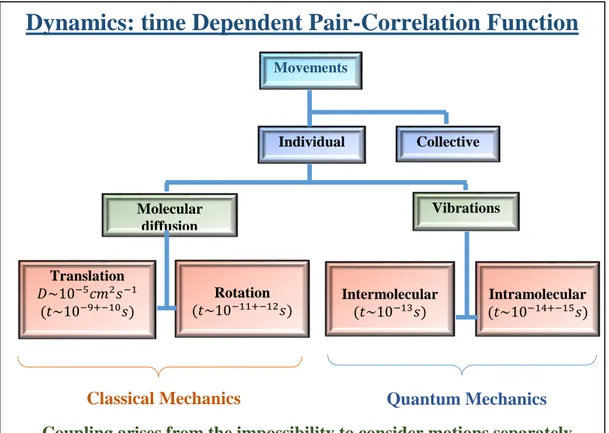
Dynamics: time Dependent Pair-Correlation Function
Coupling arises from the impossibility to consider motions separately
Movements Individual Collective Molecular diffusion Vibrations Rotation 𝑡~10−11+−12𝑠 Intermolecular 𝑡~10−13𝑠 Intramolecular 𝑡~10−14+−15𝑠 Translation 𝐷~10−5𝑐𝑚2𝑠−1 𝑡~10−9+−10𝑠
vib s rot s trans s s
I
I
I
I
(1.47))
,
(
)
,
(
)
,
(
)
,
(
Q
S
Q
S
Q
S
Q
S
s
strans
srot
svib (1.48)If the motions are independent this result implies that the total incoherent scattering law is the convolution product of the scattering laws for the three elementary motions. In fig. 1.8 a sketch of autocorrelation, cross-correlation and convolution is shown.
Fig.1.8: Sketch of autocorrelation, cross-correlation and convolution
If now the molecules have inside inequivalent protons, the equations that we saw earlier should be averaged over these protons. In this case, the spectra reflect the superposition of the motions of the different protons. A way to separate them is to use several partially deuterated specimens in order to make invisible to neutrons afterwards each kind of proton. This approach was successfully utilized in the field of liquid crystals.
1.4.6 Incoherent “Quasi-elastic” Spectra
In this part, we discuss calculations, that are simple in some cases, to make obvious the main features of incoherent spectra reflecting pure rotation, pure translation and a combination of both. Since these spectra are centered around 0, they are usually qualified as “quasi-elastic”.
1.4.6.1 Rotation and diffusion spectral contribution
Let us examine the simple case of isotropic rotational diffusion on a sphere of radius . The position of the particle is characterized by a vector (t). The probability distribution G of its orientation s is governed by the following rate equation
S r S D G t G 2 (1.49) In which:
t
Gs ,0, is the probability of finding the orientation at at time t if it was at 0at zero time
r
D is the rotational diffusion coefficient.
The solution of this equation is
, ,
4 ( ) *( 0) 0 ) 1 ( 0
l m l l m l m l t l Drl s t e Y Y G
(1.50)From eqn. (1.44) we get:
1 ) 1 ( 2 2 0 0 ) ( ) ( ) 1 2 ( ) ( 4 1 ) , ( 0 l t l Drl l S Q i s Q t e G d d j Q l j Q e I
(1.51)And by Fourier transforming
1 2 2 2 2 0 ) 1 ( ) 1 ( ) ( ) 1 2 ( 1 ) ( ) ( ) , ( l r r l s l l D l l D Q j l Q j Q S (1.52)Where the j are the spherical Bessel functions. l
The scattering law (1.52) is composed of a sharp ()peak superimposed on a broadened component (composed of various Lorentzians) whose width is of the order of a few D r
(fig.1.9), and whose intensity depends on Q. For more complicated models, it can be shown that these key characteristics are preserved. For example a () peak and
broadened components whose widths are Q-independent, but other characteristics (e.g. side peaks or humps) appear if the rotation becomes relatively free.
Fig.1.9: Theoretical incoherent neutron quasi-elastic scattering spectrum for a purely rotational diffusive motion
1.4.6.2 Translation diffusion spectral contribution
Now we consider the simple case of isotropic translational diffusion. The probability distribution G of the position s d(t) of the particle is run by the rate equation:
S d t S D G t G 2 (1.53) In which:
d d t
Gs , 0, is the probability of finding the particle at d at time t if it was at t at zero 0
time
t
D is the translational diffusion coefficient.
The solution of this equation is
Dt d d t s t e t D t d d G 4 ) ( 2 3 0 2 0 4 , , (1.54)From eq. (44) we get:
iQd t d DQt S s t e d d d d e G t Q I 0 2 0 ) ) 0 ( ) ( ( ,
(1.55)And by Fourier transforming
2 2 2 2 1 , Q D Q D Q S r r s (1.56)It was noted that the scattering law (1.56) is a single Lorentzian line whose amplitude varies like Q (figg.1.10-1.11-1.12). For more complex models, we get a superposition 2
of Lorentzian (or more complicated shapes) lines whose widths and relative intensities are Q-dependent. This must be compared with the rotational case where only the amplitudes are Q -dependent.
Fig. 1.11: Random jump diffusion
1.4.6.3 Superposition of rotation and translation diffusion spectral
contributions
The molecules are now assumed to undergo self-diffusion and reorientation. Supposing that these movements are independent, the total scattering law is the convolution of the rotational and translational scattering laws. It was noted that even if the two movements are described by simple models that we talked about, the scattering law is the sum of a number of elementary curves (Lorentzians) whose widths depend both on translational and rotational parameters and whose relative amplitudes are Q -dependent. It is therefore difficult a priori to separate the two contributions, mostly when the finite instrumental energy resolutions is regarded. Nevertheless this is now possible using the concept of the Elastic Incoherent Structure Factor (EISF) and combing measurements from various instruments, as will be seen below
1.4.6.4 Vibrational spectral contribution
Lastly, when there are vibrations, the total scattering law should be convoluted with that of vibrations, which is generally composed of sharp peaks of small intensity in the inelastic region.
In the quasi-elastic region, it can be demostrate that this affects the scattering law through
a Debye-Waller factor
2 2
u Q
e , where u2 is a mean square vibration amplitude. In this case we can write:
2 2 , , strans srot Q u quasi s Q S Q S e S (1.57)The Debye-Waller factor thus pictures the decrease of the total “quasi-elastic” intensity with increasing
Q
(i.e. the scattering angle) and povides information on the extent of the (fast) vibrational motions.1.4.7 The Elastic Incoherent Structure Factor (EISF)
We take into account the rotational scattering law (1.52). In this law the first term is the product of a function of Q , F(Q), multiplied by a ()function. This property is
in fact general for whatever rotational model and derives from the fact that Is(Q,t)does
not decay to zero wheret. We have:
Q I Q,t
G (r,r0, )e drdr0F s
S iQr (1.58)Namely, the coefficient of the () function, that has the dimension of a structure factor and is called the Elastic Incoherent Structure Factor (EISF), is the spatial Fourier transform of final distribution of the rotating proton, averaged over all possible initial position.
Since F(Q) pictures the “trajectory” of the moving proton, if F(Q) could be extracted from spectra obtained at variousQ values, one would have precious information on the nature of the rotational motion performed by the proton. The way to relate the EISF to a misurable quantity is the following: it was noted that any rotational scattering law can be written
𝑆𝑠𝑟𝑜𝑡 𝑄, 𝜔 = 𝐹 𝑄 𝛿 𝜔 + ∑ 𝑜𝑡ℎ𝑒𝑟 𝑏𝑟𝑜𝑎𝑑𝑒𝑛𝑒𝑑 𝑡𝑒𝑟𝑚𝑠
𝑛 (1.59)
Furthermore, Fourier transform of eq. (1.44) and integration over ω yields: 1 ) 0 , ( ) , (
SS Q d IS Q (1.60)Integrating eqn. (1.59), it is evident that F(Q)is the fraction of the total quasi-elastic intensity contained in the purely elastic
peak. If the instrumental resolution is (much) smaller than the reorientational rate, then the real spectra have the form sketched in fig.5, and the separation between the sharp (purely elastic) and broad components can be performed by natural extrapolation. Let Ie(Q)and Iq(Q) be the correspondingintensities (measured by graphical integration after subtraction of a flat background). We have:
) ( ) ( ) ( exp I Q I Q Q I Q F q e e (1.61)The analysis is a priori much more difficult and, in each case, less precise, if the two components are not well separated. Are now increasing in number the studies of purely rotational motions in molecular crystals based on these ideas. For example we mention the problem of reorientation in plastic crystals, in liquid crystals, and that of methyl group rotation in solid phases.
We have consideredthus far only pure rotation but when self-diffusion is superimposed on rotation (as it is in the case in molecular liquids), one can generalize.
Practically, we find that it is necessary that we know D rather accurately in order to t
extract a reliable value for the EISF and accordingly, a reliable picture for the rotation. The diffusion coefficient D can often be obtained regardless by the neutron method by t
working at sufficiently low Q (such that 2 1
rot tQ
D ) and sufficiently high resolution (such that DQ2
t
). In these conditions only the translational part is seen in practice, the rotational contribution acting as a flat background. These experimental conditions can nowadays be achieved for usual liquids (D 10t -7 cm2/sec) using the backscattering technique. After determining the value of Dt, one can make experiments on a medium
resolution instrument (such that Δ
1rot
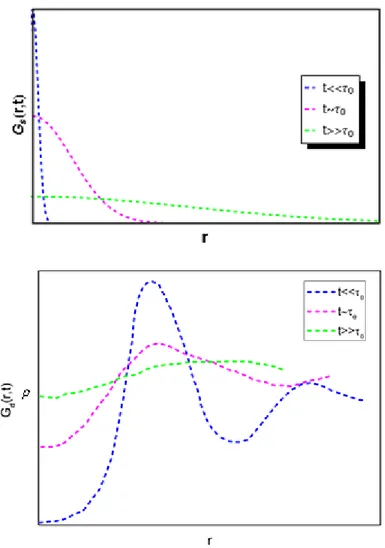
): typically 10<Δ<100 μeV and extract the EISF from these spectra to obtain information about the rotational model.In fig. 1.13 are shown graphs in which it is evident a time dependent pair correlation functions and of dynamical structure factors.
Fig 1.13: Sketch of the typical behaviour of the time dependent pair correlation functions and of the dynamic structure factor for solids, liquids and glasses
1.5 Absorption and scattering of electromagnetic waves: dielectric and
infrared absorption, Raman and Rayleigh scattering
In this part, we explain how electromagnetic (e.m.) waves or photons of long wavelength (much greater than molecular dimension) can be useful to study molecular motions [1]. First and foremost we listen the properties which characterize the photon, then we focus on the principles of absorption and scattering experiments and give a few illustrative examples.
1.5.1 Electromagnetic waves and photons
The electromagnetic field is classically characterized by its electric field vector, )
(r
E , and magnetic, H(r), field vector, and has a wave character. A plane wave is characterized by its wave vector k, its angular frequency k , and moves at the velocity
of light c. These quantities are related by
c=
k k
(1.63)
Furthermore, electromagnetic waves can be seen as a ultra relativistic particles, photons, moving at the velocity of light and of energy Ek given by
Ek=k (1.64)
For visible light, we have Ek2eV and λk6000 Ǻ. So is interesting put these values
in comparison with the corresponding ones for neutrons, in particular the fact that the wavelength is much greater than the usual molecular dimensions. In fig. 1.14 the photon’s “identity card” is reported.
Fig. 1.14: The photon’s “identity card”
Considered the electromagnetic field as a quantum object, it must be treated as an operator within the formalism of second quantization:
k k E k c k E k c E * (1.65) k k H k c k H k c H * (1.66) where 2 exp(ik r) V i E k k (1.67) and k Ek k k H . (1.68)
k=clk is the angular frequency
cl the light velocity
k the wave vector
the polarization versor
V is the volume of quantization and the annihilation and creation operators respectively.
The eigenstates Nk of the Hamiltonian of the field are characterized by the number
k
N
of photons existing in each state (k,μ)... ,..., , , 2 , 2 1 , 1 k kpp k k N N N N (1.69)
The corresponding eigenvalues are
E= k k k N
, , ) 2 1 ( (1.70)Finally, the properties of the operators ck,μ and c+k,μ are:
ck,μ Nk'' = Nk Nk 1kk'' (annihilation of one photon kμ) (1.71)
c+k,μ
' '
k
N = Nk 1 Nk 1kk'' (creation of one photon kμ) (1.72)
1.5.2 Long wavelength e.m. waves- matter interaction
Electromagnetic waves interact with electric charges. If the medium is neutral, at each point r, one can define a permanent dipole moment u(r), a polarizability tensor
) (r
per unit volume. If the wavelength is enough large, it can be see that the interaction Hamiltonian can be obtained by an expansion in the electric field:
𝐻𝐶 = − ∫ 𝑑𝑟 [𝐸 𝑟 𝜇 𝑟 +12𝐸 𝑟 𝛼 𝑟 𝐸 𝑟 + ℎ𝑖𝑔ℎ𝑒𝑟 𝑜𝑟𝑑𝑒𝑟 𝑡𝑒𝑟𝑚𝑠] (1.73)
The interaction with the permanent dipoles is taken into account by the first term
(r
)
, and the interaction with the induced dipoles by the second term
(
r
)
E
(
r
)
when
(r
)
being the polarizability tensor.The higher order terms include the hyperpolarizability interaction (trilinear term in the electric field), magnetic interactions, etc. For what interests us, we will restrict ourselves to these two first terms which will lead to dielectric and infrared absorption (linear term) and to Rayleigh and Raman scattering (bilinear term).
The Fig. 1.15 shows the wavevector-energy region accessible for photons.
Figure 1.15: Photon accessible wavevector-energy region
1.5.3 Dielectric and infrared absorption: interaction with permanent
dipoles: Introductive definitions
We must first of all say that:
the probe is the e.m. field whose eigenstates are ;
the reservoir is constituted by N particle which we suppose to be point-like, located at ri (long wavelength approximation) and characterized by their dipole moment μi. With
this assumption, we can write
i i i r r r) ( ) (
(1.74)and the present relevant interaction HC (first term of eq.(73) is written:
V i i CE
r
r
r
r
d
r
H
(
)
(
)
(
)
(1.75)using eqn. (1.67) in eq. (1.75) and performing the integration over r yields
k N
i ikri
k r k i k i k k i Cc
e
c
e
V
i
H
,2
)
(
(1.76) Now we have to calculate the average value ofH
Cbetween the initial and final state of the probe, that we callH
C. The initial state isN
k I0 , i.e. are sent on the sample
photons of momentum k0 and polarization εI (a monochromatic and polarized plane
wave). Now let's see what are the possible interesting final states, i.e. those for which
C
H
has non-zero value. They correspond, obviously, to states such that the matrix elements of ck,μ or c+k,μ are non zero. According to eqs. (1.71) and (1.72) these are:(i)
1
0I
k
N
:absorption of one photon (k0, εI)(ii)
1
0I
k
N
: emission of one photon (k0, εI)(iii)
N
k I k s1
0
,
1
: emission of one photon (k1, εs)The values of the matrix element are
N
k I0
N
k0I
1
and 1, respectively, and thecorresponding probability of transition is thus proportional to
N
k0I ,1
0I
k
N
and 1.If the number of incident photons is big, as always happens in practice, then
N
k I0 >>1
and the the last case (in fact the spontaneous emission) is very weak compared to the two former ones, i.e. the induced absorption and emission. The correlation functions corresponding to these two latter cases are:
( ) (0) , 0 ) ( 0(
(
))(
(
0
))
02
i i C C r t r k i j i I i I i I k t H HN
t
e
V
C
(1.77)with + for absorption and – for emission.
It was found that, a priori, the study of induced absorption and emission of e.m. waves by such a medium can provide information regarding the motions of μi (rotation and
vibration) and on the motion of ri (i.e. translation). Pratically, however, k0 having a very
small value (long wavelength approximation), the exponential decays much more slowly compared to the other terms and we can neglect its variation. With the conditions listed, the correlation functions for emission and absorption are the same, and we have:
j i I i I i I kt
N
V
C
t C H C H , 0(
(
))(
(
0
))
2
0 ) (
(1.78)Eqn.(1.17) provides the corresponding probabilities of transition, one with ω=ω0
(absorption of one photon), the other with ω=-ω0 (emission of one photon). These two
probabilities are related by eqn. (1.18) in the linear approximation and we have Wabs Wemi. As foreseen by the general considerations, the net induced phenomenon is the absorption and the corresponding probability per unit time is according to eqns. (1.16), (1.17), (1.18) and (1.78):
1
(
)
2
0 2 ( )
t C H C HC
e
W
W
W
t obs emi
(1.79)Considered a sample that is a cylinder of section S and length l (Sl=V). The problem is now to relate Wt to a measurable quantity, namely the power Pa absorbed during the
experiment. Let P0 be the incident power and
n
k I0 the corresponding incident number
of photons per cm2 and per sec. We have:
P0=
n
k I0 S
0 (1.80)The number of incident photon in volume V is
I k
N
0 = V c nk I 0 (1.81)As the power absorbed in volume V is
Pa=
0W
t (1.82)Combining eqn. (1.78) to (1.82) we finally obtain
1
(
)
)
2
(
0 0 2 0 0
c
e
S
c
N
P
P
a
(1.83) withdt
e
t
c
c
it
(
)
2
1
)
(
(1.84) and
j i I i I jt
N
t
c
,)
(
)
0
(
1
)
(
(1.85)It was found that, in the long wavelength approximation, the absorbed power is proportional to the spectral density of the fluctuation of the dipoles. Specifically, it reflects the correlation between the fluctuations of the components of the dipoles along the polarization
I of the field. We have an important simplification if the medium can be considered as isotropic (e.g. as in a normal liquid). Then, one can average eq. (1.85) over all possible orientations of
I and easily obtain:
j i i jt
N
t
c
,)
(
)
0
(
1
)
(
(1.86)We highlight the fact that the electric dipole moment of a molecule is a quantity which depends on the charge distribution in the molecules and this distribution changes when the molecule vibrates. We denoted by υ the vibrational states and by qυ the corresponding normal coordinates. We can write:
0
q
(1.87) with 0
qq
(1.88)μ0 is the permanent dipole
μν is the derivative dipole corresponding to vibration ν.
According to these definitions, we have that the second member of eqn.(1.85) or (1.86) can be subdivided into various components (two for eqn. (1.86)):
j i i jt
N
t
c
, 0 0 00(
0
)
(
)
1
)
(
(1.89) and
1
(
(
0
)
(
)
)
(
(
0
)
(
))
)
(
' , , ,t
q
q
t
N
t
c
j i j i i j vv
(1.90)which are respectively: the relevant correlation functions for the so-called dielectric and infrared absorption in an isotropic medium. We have illustrated in detail later of these two cases.
1.5.3.1 Dielectric absorption: permanent dipoles
a) General
By eq. (1.89) we have the correlation function. If we consider identical molecules, considered ui and
u
j the unit vectors along0
i
and 0
j
, and
i,j the angle betweenthem, eq. (1.89) the equation becomes as follows:
j i ij t N t c , 2 0 00 ( ) cos( ( )) 1 ) (
(1.91)This correlation function shows the fluctuations of the relative orientation of the permanent dipoles and thus reflects collective reorientational motions. A difficult problem is to relate this macroscopic function to monomolecular properties, namely to the single molecule correlation function F1(t) given by
F1(t)= P1 cos(ii(t)) (1.92)
where P1 is the first order ordinary Legendre polynomial. It is possible to address the
problem experimentally using a trick: should be diluted polar molecules in an inert solvent and make a study as a function of the dilution. If the dilution is sufficiently large, the active molecules can be considered sufficiently far from one another so that their correlations can be neglected i.e. that we have:
0
))
(
cos(
ijt
for i j (1.93)In this case, Eq. (89) can be written dropping the indices ii: ) ( ) ( ) ( 1 2 0 00 t F t c
(1.94)and by Fourier transforming ) ( ) ( ) ( 1 2 0 00 t
F
c (1.95)Using the fact that
(i) in dielectric absorption 0 kBT and
(ii) N=nSl where n is the number of dipoles per unit volume, We can write eqn. (1,83) as:
0
lP
Pa (1.96)