Managerial assessment of Italian airport efficiency: a statistical DEA approach

Testo completo

(1)Managerial assessment of Italian airport efficiency: a statistical DEA approach Claudia Curia, Simone Gittoa, Paolo Mancusoa*.. a. Facoltà di Ingegneria, Dipartimento di Ingegneria dell’Impresa, Università di Roma “Tor Vergata”. Via del Politecnico, 1, 00133 Roma, Italy. e-mail: curi@disp.uniroma2.it; gitto@disp.uniroma2.it; mancuso@disp.uniroma2.it * corresponding author. Phone: +39-06-72597793 Fax: +39-06-72597305. Abstract We estimate the technical efficiency of a sample of Italian airports over the period 2000-2004, using a bias-corrected DEA estimates (Simar and Wilson 1998, 2000 and 2002). Two models “physical” and “revenue” are used to gain managerial insights about the areas of inefficiency. The results show a technology characterized by constant returns to scale, an increase merely in revenue efficiency and different benchmarks according to the model used. The joint analysis of the two models through a scatter plot matrix identifies three groups of airports: two of them are mostly operational inefficient, while one boasts the leadership in managerial efficiency.. Keywords: Airport efficiency, bootstrapping-DEA, return to scale, Italian airports. JEL Classifications: L93; C14;D24; L51.. 1.

(2) 1. Introduction Since the mid-1980s, the worldwide air transport sector has been characterized by significant structural, institutional and regulatory changes. In particular, the deregulation policies in the air transport services, started in US after the mid-1980s and followed by Europe at the end of 80s, were designed to foster competition in both domestic and international markets and to enhance carriers’ performance (Oum and Yu 1995). At the same time, most governments have adopted policies whose effects have impacted on airport management and ownership structure. Commercialization and privatization of airports have become the worldwide trend (Oum and Yu 2006), although the processes of implementation have been very different and heterogeneous among countries. The common aim of governments in promoting airport privatization includes a desire to remove airports from the public sector, increase capital investment in existing airports, protect airport administration from political interference and impose commercial disciplines on airport management (Lin and Hong 2006). The Italian scenario has been permeated by deeply institutional changes, enabled by national and European directives. Such directives proposed changes for concession agreements, government and entrance of private capital in the airport management companies. In turn, these institutional forces have set up high standards to the diffusion of mixed private-government ownership and the disappearance of 100% government corporation ownership. In this new context, the need to intensify the monitoring of airport performance by investors and governments has been risen. In general, performance measures are helpful in policy decision making to choose the best framework to organize the airport system as they provide meaningful insights across the airports, identify the best performers and determine the main variables that impact on airport performance. The airport performance is measured in terms of its productivity and efficiency level. Given that, the efficiency analysis of airport industry has been becoming a “hot” topic and it is handled as a general methodology in evaluating the effects of regulatory reform on airports’ performance. Many scientific papers have been published on the airport performances but there is still room for further research. Indeed, most of them have focused on productivity and efficiency analysis of US and major international airports (Gillen and Lall 1997; Sarkis 2000; Martin and Roman 2001; Pels et al. 2001; Oum et al. 2006), omitting the role played by regional airports in attracting air-transport services operated by low cost companies. Moreover, there are few papers dealing with the Italian airport industry, some of which take into account only the two Italian systems (Roma and Milano). Barros and Dieke (2007, 2008) propose two studies to empirically address the operational and financial efficiency of the Italian airports sector, investigating also for the main drivers of the inefficiency, by using a the two stage procedure based on bootstrap (Simar and Wilson 2007).. 2.

(3) Although their innovative approach, certainly accurate from an econometric point of view, both papers suffer from some pitfalls. The drawbacks concern the lack of an accurate (a) choice of the variables to use, in terms of endogenous and exogenous variables with regard to the production problem, (b) characterisation of the airports (in terms of public vs private) and (c) analysis of the efficiency estimates (in terms of sensitivity to the sampling variation), with the consequence of non-robust policy implications. The contribution of this study is to fill this gap, providing a meaningful assessment of technical efficiency for the Italian airport sector. In particular, the paper extends the mere efficiency analysis to a more accurate framework, in terms of statistical and managerial viewpoint. The technology frontier characterization is provided, in terms of returns to scale, as well as the corrected bias estimation and the uncertainty about each airport efficiency. To provide more useful insights to the decision makers, the efficiency is analyzed under two different perspectives prospective (operative and financial) which reflect the objectives set by the airport management companies after the privatization process. In what it follows, we first describe the Italian airports industry (section 2), then we briefly describe the methodology adopted (section 3) and the data selected (section 4). In section 5, the results of the efficiency are presented and finally, section 6 contains some concluding remarks.. 2. The Italian airport industry Since 1987, significant policy developments have affected the European airport industry, enforcing a set of liberalization and privatization measures. The Community’s airport industry has undergone fundamental organizational changes that have reflected the reassessment of the government’s role played in the airport sector and the aim to enhance managerial incentives in private enterprises and to sever the link between managers and politicians (Gönenç et al. 2001). In Italy, the airport reform process has been very slow to go along and difficult to implement due to the fact that four actors have been involved. The State, as owner of lands and infrastructures, the management companies (both public and private), the control organism, ENAC1, and the carrier companies. Moreover, the existence of special laws and different concession agreements have been sources of heterogeneity in the airport governance forms. Indeed, since the mid-1950s, only some airport management companies as those of Genova (GOA), Milano Linate (LIN), Milano Malpensa (MXP), Roma Ciampino (CIA), Roma Fiumicino (FCO) and Torino (TRN) are in charge for the provision of all airport’s services (airside and landside), by special laws2. They collect revenues derived from all airport 1. ENAC, a public authority, has the trusteeship for the airports side by the State and exerts activities for technical and management control on the airport activities. Moreover, it issues the concession agreements to the airports (see further). 2 Genova (GOA) law n. 156/1954; Milano Linate (LIN) aw n. 194/62; Milano Malpensa (MXP) law n. 449/85; Torino (TRN) law n. 14/65, n. 736/86, n. 187/92; Roma Fiumicino (FCO) law n. 775/73, Roma Ciampino (CIA) law n. 985/77 and Venezia (VCE) Law n. 938/86.. 3.

(4) operations and services, are responsible for the whole infrastructural development and they are subject to a contractual liability to pay a concession fee to the State for land use. This form of concession agreement, known as “Totale” (T), assigns to the management companies the right to use and manage the airport land for a 40-year period. Other forms of concession agreements are represented by the “parziale” (P), “parziale precario” (PP) and “diretta” (D). In the P agreement the management company provides services for aircraft (taxiways, apron areas, fire fighting, etc), passenger and freight (security cleaning, etc.). The company is responsible for non flight airport infrastructures (aerostation, car-parking, etc) and receives revenues from passenger handling charges. The remaining infrastructures are managed by the State which derives revenues from all the remaining aeronautical charges. The PP agreement usually precedes the P and differs by the fact that the State receives all the aeronautical revenues. Finally, in the D agreement all the activities are managed by the State. Starting from 1999, the airports can obtain a Total concession from ENAC through a long process of eligibility requirements (see Tab. 1). Moreover, as far the privatisation process is concerned, the Italian law n°35/1992 has had a great impact in reforming capital structure of airports. In fact, most of them have been privatized but, only few are under a majority private ownership. Looking at Table 1, three stylized facts might be observed: •. the absence of any systematic tendency between high values of ROI and the type of ownership structure: private vs public;. •. the influence of agreement type in the revenues composition;. •. the scarce capacity of the airports characterized by less than 1.5 million of passengers to generate returns on the invested capital.. Although the heterogeneity in the production process among airports, some common elements characterized them. The first one is the concession agreement which, as explained above, impacts on both costs and revenues structures. In particular, revenues are strongly affected because their components, such as tariffs and taxes connected with the services for airports operations, are determined by the Minister of Transport and Finance through a complex formula which includes variables related to traffic, productivity growth rate, infrastructure development, service quality, etc. The second one concerns the handling services. The most important changes on the handling services liberalization have been driven by the Italian law n.351/95 and the European directive 96/67/CE. The first law has allowed airport management companies to exploit the possibility, but not the duty, to give in outsourcing handling services to external companies; the second law has enforced the Italian law since January, 1st 2001 and liberalised the ground handing with more 3 million passenger or 75,000 tonnes of freight3. This directive has had an impact only on the main airports, excluding the secondary ones. Lastly, the. 3. Or greater than 2 million passenger movements or 75,000 tonnes of freight during the six-month period before April of the previous year.. 4.

(5) phenomenon of the low-cost carriers has constituted a large growth opportunity for small airports by increasing in passengers’ movement from and to them. In general, the entire system has undergone important changes which have partially damped the strong Italian polarized structure in the two systems of Roma and Milano (Bernardi 1983). Indeed, since the end of 1970s, more than 50% of the passenger traffic was absorbed by them. After the liberalization process, this percentage has been held constant although the increase in traffic demand, proving that the increase in passenger demand has been absorbed by secondary airports (Ferrario 2006). Turning to the composition of the sector, the Italian airport industry is constituted of 101 airports; among them only 45 contribute to the amount of generated traffic and relative commercial activities (ENAC 2005). Our sample includes up to 18 airports, shown in Table 2, and covers on average 89.9%, 95.6% and 83.6% of total number of passengers, cargos and movements registered in Italy from 2000 to 20044. Following the airport classification based on traffic volume, our set contains 13 airports with more than 1.5 million of passenger movements and 5 regional airports, where mainly operate low cost companies. Some airports serve mostly international traffic, such as CIA, FCO, MPX and BGY whereas others serve mostly domestic passengers (e.g. LIN, NAP, PMO, TRN, see Table 2). Moreover, some airports face high fluctuation in served traffic, measured by ratio between maximum and minimum value of WLUs, caused by seasonality in passengers’ demand. Inside each group, both volume and growth rate for traffic served is very different. in particular, CIA has shown an average increase by 40% while BGY 50% in the international passengers. The two hubs, Roma Fiumicino and Milano Malpensa have shown, respectively, 3.11% and 0.04% growth rates. As far as the domestic traffic is concerned, there have been small variations in the entire Italian system, expect for Milano Malpensa (-10.4%) and Roma Ciampino (32.7%), pointing out their orientation towards international traffic. Generally speaking, the polarized structure of the entire Italian system persists over the period of analysis but, at the same time, smaller airports are absorbing the increase in traffic volume, outlining a new way of making business and supporting the regional development. From the above tables, it can be noticed that the Italian airport infrastructure is characterized by a peculiar structure that distinguishes it from the rest of European airports (OECD 1998): it is constituted by a high number of small airports wide spread over the country, different in nature and volume of served traffic, business and governance structure.. 4 The total number of Italian passengers, cargos and movements does not include those airports devoted to the regional and commercial aviation, characterized by less than 150 000 passenger movements (ENAC).. 5.

(6) 3. Methodology The technical efficiency is estimated through non parametric technique, the Data Envelopment Analysis (DEA): it is based on the measurement of the distance of each Decision Making Units (specifically the Italian airport) to the estimated technology frontier, defined using linear programs (Charnes et al. 1978, Fare et al. 1985)5. The popularity gained by DEA-estimator in the field of measurement of technical efficiency is attributable to some of its appealing properties: it requires only the typical, and “innocuous”, economic assumptions (Shepard 1970; Fare et al. 1985), does not rely on any assumption on the analytical shape of the underlying technological frontier and it is very flexible because it handles multi-input and multi-output setting. We focus our analysis on the estimation of the technical efficiency, that is the measure of airport ability to obtain the maximum output from a given set of input and technology. We use an output-orientated model as it ensures to account the objective of exploiting the facilities to satisfy the steady growth demand in aviation market (Martìn and Romàn 2001). In order to ease the interpretation, we express the technical efficiency in terms of Shepard (1970) distance, which is bounded between the zero and unity (the best technical efficiency estimated). It is derived by the reciprocal of Farrell (1957) distance, given by:. [ { (. ) }]. ˆ ) = sup λˆ : x , λˆy ∈ Ψ ˆ , Dˆ ( x , y Ψ. (1). ˆ is the estimated production set, x ∈ ℜ H and y ∈ ℜ K are the input and output where the Ψ + + vectors and λˆ the estimated Farrell distance. Nonetheless, DEA-estimator shows some statistical properties which, if not accounted, lead to erroneous conclusions in the empirical investigation. As noted by Simar and Wilson (1998, 2000), the traditional DEA-estimator is biased by construction (upward and downward, respectively, for input and output orientation), is affected by the uncertainty due to sampling variation and suffers of the curse of dimensionality6. To attack empirically any of these DEA-estimator drawbacks, different statistical tools are applied. This enables to provide a more accurate and less possible biased analysis of the technical efficiency that, at the best of our knowledge, has never been carried out by other studies in the airport performance measurement. We apply the procedure proposed by Simar and Wilson (1998, 2000) to derive the sampling distributions of the DEA-estimator. It is based on the bootstrap technique (Efron and Tibshirani 1993) in a Monte Carlo setting. For any unit, it assesses the uncertainty about the technological efficiency (i.e. the distance) from its allocation to the real technological frontier, providing the. 5. Details of DEA have appeared everywhere so here are not reported. However, for more details see Charnes et al. 1978, Fare et al.1994; for a recent survey it is possible to read Cooper et al. (2007) or Thanassoulis et al. (2008). 6 It reflects the property of consistency of the DEA-estimator (see for details Kneip et al. 2007).. 6.

(7) range of variation (i.e. confidence interval) and correction for the bias term (Simar and Wilson 1998, 2000). In comparison with the traditional DEA, widely applied in the airport performance, technical efficiency is evaluated in terms of interval estimates rather than of point estimates. The main idea is to estimate its sampling distribution of the technical efficiency by using iteratively (B times) a consistent bootstrap. It consists in simulating the Data Generating Process (DGP) by resampling the efficiency estimates expressed by the kernel density estimator, bearing in mind its severe bias near the boundaries of support (in 0 and 1)7. Then, it derives the pseudo sample of input and output and compute the pseudo DEA-estimation. Once the Monte Carlo realizations are computed, the statistical inference is easily derived. Thus, for the generic unit i,. ( ). compute the bias term BIAS λî = B −1. N. ∑ λˆ b =1. * i ,b. − λî , ∀ i = 1,..., N , where λˆ*i is the. bootstrapped technological efficiency and N is the number of units; and compute the biascorrected estimator λˆci = λî − BIAS (λî ) = 2λî − B −1. B. ∑ λˆ b =1. * i ,b. 8. Lastly, it estimates confidence. intervals of technical efficiency λî + α α* ≤ λi ≤ λî + β α* , where α α* and β α* are the quartiles of the Monte Carlo distribution. The above procedure, called Smooth Homogenous Bootstrap, is applied since it enables to make inferences about the true levels of efficiency. This approximation of the sampling distribution is proved to be consistent by Kneip et al. (2007). In our case, the sample is composed by 16 observations (see section 4) and we propose two production models (see section 4): in the first model, the production process is described in a six dimensional-space (three inputs and three outputs) while in the second one, we have five dimensions (three inputs and two outputs). As far as the curse of dimensionality is concerned, rate of convergence for DEA estimator has been proven, at least for variable returns to scale (Kneip et al. 1998). Indeed, as Simar and Wilson (2008) claim: “the number of observations need to increase exponentially (not proportionally) respect to the number of inputs and outputs to maintain the same order of estimation error”. It means that the use of several "rules of thumbs", based on proportional increase in the number of observations, does not have statistical sense. Thereby, to preserve the speedy of the convergence rate and avoid additional noise to the estimation, we aggregate the input and output vectors. For both models two proxy factors, which best summarize the information hold by all input and output variables, are computed reducing the dimensional space from six (or five) to two (i.e. one input and one output). At this purpose there are several multivariate statistical tools (Simar and Wilson 2008). Due the high level of correlation among. 7. To overcome this problem, the authors applied the method of reflection proposed by Silverman (1986). The correction should be when the bias correction introduces additional noise to the original point estimates (Efron and Tibshirani 1993).. 8. 7.

(8) the variables9, the procedure proposed by Daraio and Simar (2007) is applied and the two proxy factors are computed by a linear aggregation of the input and output vectors, using the first eigenvector of greater eigenvalue of the input (or output) matrix as weight coefficients. Moreover, attention has been devoted to the technological frontier. Indeed, we test the hypothesis of Global Returns to Scale –Constant (CRS), Non Increase (NIRS) or Variable (VRS)- using a formal statistical test, proposed by Simar and Wilson (2002). It is a two step test (it tests CRS against VRS, if the null hypothesis is rejected, then test NIRS against VRS), where the test statistics10 is given by the typical scale efficiency term and the p-value by the approximation (using Monte Carlo experiments) of the average number of times the bootstrapped scale efficiency is less (or equal) to the estimated scale efficiency term. We use FEAR package (Wilson 2007) for R software to compute DEA estimates. The results throughout this paper are obtained from 2000 bootstrap iterations. We employ the CrossValidation method for the choice of the bandwidth and the results appear robust with respect to variations11.. 4. Data In this study the efficiency evaluation is assessed to provide a managerial tool that enables to (a) monitor and improve aspects of the operational performance by reference to, and learning from, other organizations (Francis et al. 2002), (b) compare a set of different airports to improve their competitive position through the identification and adaptation of best practise (Graham, 1999, 2001). Thereby, technical efficiency is estimated using two different models: Physical Model where it is expressed as function of airports characteristics variables, following Sarkis (2000); Revenue Model where it is expressed as function of economic variables, following Fernandes and Pacheco (2003). The first model emphasizes the ability in managing operational processes and airport capacity, in terms of exploitation of the resources used, while the second one, the ability in capitalizing the advantages given by reformed system, in terms of exploitation of the diversification strategy. The results are jointly discussed by a scatter plot matrix (Fernandes and Pacheco, 2003), as each airport could, for instance, achieve high level of revenue from non aeronautical service and, at the same time, low level of capacity exploitation. Given this aim, the input and output variables are selected among the resources common to all airports (and used by other authors) and self reported in annual reports. Nonetheless, we classify. 9. Correlations between the variables is always greater than 80%. All tables are available from authors upon request. Simar and Wilson (2002) try several statistics in a Monte Carlo experiment. They found that a statistic given by the ratio of means of DEA-CRS and DEA-VRS scores, performs very well. So we use the same statistic. 11 We check the robustness of the results setting the bandwidth h at 0.5 and 1.5 times the previous value. All tables 10. are available from authors upon request.. 8.

(9) them into physical and financial variables (input and output), to characterize the production process by the managerial prospective, after the liberalization. Three sources are used: balance sheet of each airport, Traffic Data of Assaeroporti12, and Annual Statistics from ENAC (20012005). The Physical Model measures technical efficiency by capturing the effects of operational strategy with regard to the airside activity13. Thereby, labour, number of runways and apron dimension are chosen as input variables while number of movements, passengers and amount of cargos as output variables. The labour variable is measured by the number of employees who work directly for an airport (Oum et al. 2003). The number of runways is simply measured by the sum of total of runways. It is used to provide a better estimation of the airport dimension rather than the runway length should give since the disappearance of the distinction between national and international runways (Pels et al. 2003; Sarkis and Talluri 2004). Finally, the apron dimension, expressed in square meters, is assumed to be a good proxy to measure the operational and service aspects of the airside. Indeed, it is that part of any airport intended to aircraft operations (manoeuvring, refuelling, servicing, maintenance, parking and movement of aircrafts) and passengers and cargo service (loading and unloading). On the output side, the number of movements is measured by both takes-off and landing movements (ENAC, 20012005), the number of passenger movements is measured by the sum of passengers arriving (or departing via commercial airplane) and those passengers stopping temporarily at a designed airport (Sarkis and Talluri 2004). Finally, the amount of cargos (expressed in tons) is added to the analysis because of its increasing impact on many Italian airports. Differently, the Revenue Model measures the technical efficiency by capturing the effects of the strategy of diversification with regard to airside and landside activities. Labour cost, other costs and airport size are taken as input variables while aeronautical and non-aeronautical revenues as output variables. It is worth to note that we follow the accounting system of the airport for the definition of input and output variables (as occurred in other studies: e.g. Oum et al. 2006). The labour cost variable is measured as the cost of labour, taken from the annual balance sheets. Following Oum et al. (2006), the “other costs” variable is chosen to measure all the expenses not directly related to capital and personnel and reflects also the expenses on the airports’ outsourcing activities. It accounts the effects of the diversification strategy with respect to the outsourcing activities. On the output side, the classification of revenues in aeronautical and non aeronautical is respected. The inclusion of non aeronautical revenue as output variable removes bias in efficiency estimates, otherwise underestimated in those airports with more proactive. 12. Assaeroporti is the lobby of management companies. www.assaeroporti.it. The analysis is restricted to the airside activity since the lack of data regarding the landside cross time and airports. The number of gates and/or terminal should be good variables to measure technical efficiency of the landside activity, but, unfortunately, here it is not included due to the lack of complete data across the panel. 13. 9.

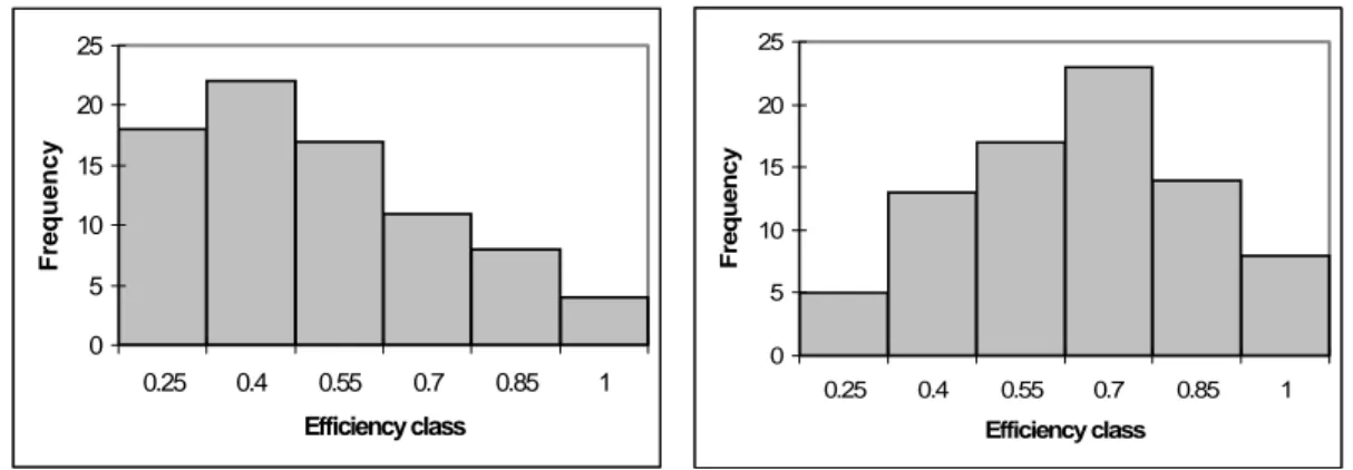
(10) managers focused on exploiting the revenue generation opportunities from non aviation business. In our sample, for some airports non aeronautical revenue generates high portion of their total revenue (e.g. 45.7% for CIA_FCO and 44.4% for GOA, see Table 1). It is worth to note that two couples of airports with the same management company (Roma Ciampino-Roma Fiumicino and Milano Linate-Milano Malpensa) provide only aggregated balance sheets. This implies that they enter in the analysis as single unit, CIA_FCO and LIN_MPX, respectively so that our panel is composed by 16 observations for 5 years. Table 3 and 4 report the descriptive statistics on the variables used in each model.. 5. Estimation and analysis. 5.1 Preliminary results The composition of our data set in terms of number of observations and variables imposes, as pointed out in the previous section, the aggregation of the input and output variables (for each model in each year) into two proxy factors. The investigation of returns to scale (see Table 5) enables to assume constant returns to scale for the underlying technology; indeed, we fall to reject H0 hypothesis at 5% confidence level for both models. These results provide the first insights on the technology underlying the production process of the Italian airports and can not be compared with results from other studies, since the lack of similar investigation. They point out that the airports of our sample work at the maximum average productivity and the sources of inefficiency are attributable only to the management policy and not to the deficiency of the scale14.. 5.2 Efficiency and Sensitivity results The estimated efficiency scores obtained by the bootstrapped DEA show a substantial bias that should not be neglected15 (see for details, e.g. Efron and Tibshirani 1993 and Simar and Wilson 1998, 2000). Thereby, we adopt the corrected DEA estimates as point estimates of the technical efficiency for the discussion of results. On average, corrected DEA estimates reveal that the Italian airport system appears to be more totally technically efficient by a revenue viewpoint (overall mean equal to 0.521) than by physical viewpoint (overall mean equal to 0.395), in the sense that airports lie, on average, closer to the efficiency frontier if evaluated under the revenue prospective. Moreover, the distribution of efficiency scores differs between the two models. Looking at the frequency. 14. It does not mean they are at the optimal scale size since it depends on the input and output prices (Banker, 1984). 15 We omit the results for brevity. All tables are available from authors upon requests.. 10.

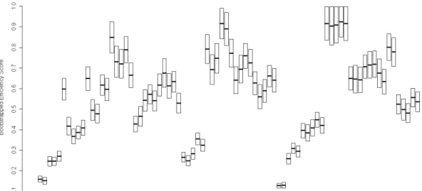
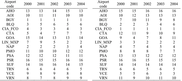
(11) distributions16 (Figure 1 and 2), in the Physical Model the efficiency scores show a more evident left skewness than in the Revenue one. Such a huge diversity might be attributed, firstly to a backward management of the airside capacity that encumbers the increase in efficiency, and secondly to the ability to quickly stem benefits from the governance reforms. Looking at the impact of the concession agreement, (Table 6), the airports with T concession show better result for both models on average. In fact, it can be noticed that more restrictive is the concession agreement form less is the airport efficiency. For the Physical Model differences between T and P concession are slightly. Yet, considering the point estimates, additional useful insights are provided by the respective rankings, depicted by Tables 7 and 8. They allow identifying stable benchmarks for improving the poorly performing airports and providing good managerial implications (Sarkis and Talluri 2004). The tables show stationary rankings for most airports in both models: few airports change drastically their positions over time. In the Physical Model, CTA gets worse ranking passing from fourth to seventh position in 2002 but preserving it stable over the last years. LIN_MPX, instead, shows a decrease in ranking in 2001, followed by a great retrieval, levelling off in second position over the last years. In the Revenue Model, GOA ranks the fourth position in 2001 and then gets worse till achieving the eleventh position while NAP undergoes a downturn in 2001, resuming its position over the remains years. On the other hand, some airports have not changed their ranks over the five-year period: BGY for the Physical Model and CIA_FCO and SUF for the Revenue Model. Both BGY and CIA_FCO are at the top ranking for the entire period. Turning to the sensitivity analysis, a more “sensitive” assessment might be found in terms of intra and inter airport performance. Differently from the previous assessment, based on the attended values, here we add more information about the variation of each efficiency estimates (at a 95% level of confidence). Fig. 3 and 4 show confidence intervals for the efficiency scores in 2000-2004, constructed with the bootstrap procedure. For instance, in the Physical Model the findings show a high variability (i.e. wide confidence intervals) of efficiency estimates around different means (i.e. staggered confidence intervals) over time for the airports of BLQ, LIN_MXP, NAP and CIA_FCO. Moreover, for some units (such as BLQ, CTA and TRN, which rank from the 5th to the 8th position in the point estimation, Table 7) differences in efficiency scores are not statistically significant. The same is valid in the Revenue Model for instance, looking at CIA_FCO and LIN_MXP in 2000, 2003 and 2004. Thus, interval results confirm only some of rankings produced by the point estimation and an accurate benchmark might be found. In the Physical Model, BGY is one of the best performer. Its confidence intervals range from an upper bound, constant over the five periods, equal to 0.996 to a. 16 The set width of each class has been chosen taking into account the smaller upper bound among those related to the best performer (BGY and CIA_FCO, respectively, for the physical and revenue model) over the five years.. 11.

(12) minimum lower bound equal to 0.734 (in 2003). This implies that BGY likely achieves highest levels of efficiency and its performance is likely to worsen in the last three years (due to the lower values of lower bound). Moreover, in comparison with the other peers, its performance is quite not statistical different from BLQ and NAP in 2000 and NAP and CIA_FCO in 2001 and 2002. It appears to be the best significant performer only in 2003 and 2004. On the other hand, in the Revenue Model CIA_FCO is one of the best performers. Its confidence intervals range from an upper bound, constant over the five periods, equal to 0.998 to a minimum lower bound equal to 0.811 (in 2001). In comparison with other peers, its performance is quite not statistical different from BLQ, LIN_MPX and NAP in 2000, BLQ, LIN_MPX and VCE in 2003 and VCE in 2004 and NAP. Only in 2001 and 2002 CIA_FCO appears to be the best significant performer .It follows that the benchmark for each model in each year is composed by a set of airports, instead of a single airport (as in the point estimation), as reported in Table 9. For the Physical Model, it is worth to note a general declining trend in the efficiency as show by the downwards shift of the confident intervals. Additionally, some airports (CTA, NAP, VCE and VRN) vary drastically the range of their confidence intervals. Only LIN_MPX improves its efficiency, denoted by an upward shift of the confidence intervals while BGY appears to hold the efficiency stationary. On the other hand, the worst performers (AHO, AOI, GOA, PMO, PSR, PSA) show less variability of their efficiencies due to narrower confidence intervals. The efficiency scenario depicts by the Revenue Model is completely different: for most airports, the confidence intervals show a upwards tendency. Only AOI and CTA decrease in efficiency while CIA_FCO seems to be stationary.. 5.3 Strategic Analysis Considering the new airport governance paradigm, a strategic analysis for the airport competitive arena might provide helpful insights to the management. Thus, here the bias corrected estimates are jointly analyzed, in terms of geometric mean, by a scatter plot matrix (Fernandes and Pacheco 2003) over the period 2000-2004 (Figure 5). In the same matrix, the forms of concession agreement enjoy by any airport are shown. The bi-dimensional visualization allows the positioning of the airports within the four quadrants. The first quadrant contains the “HH”17 airports. They represent the airport class able to guarantee long-run opportunities for both growth and profitability for the entire Italian airport system. Most of the airports with a T concession are in this quadrant. They are efficient from a revenue point of view but operate with little inefficiency in the process management. Thus, they boast leadership positions inside the competitive arena but, at the same time, need for continuous investments and further spending to defend their dominant positions and maintain their growth. This airport class is composed by BGY, BLQ, CIA_FCO, CTA, LIN_MPX, NAP. 12.

(13) and TRN. In particular, BGY could be considered as benchmark for airports devoted to taking off/landing of low cost carries. It is becoming, together with CIA, one of the most important Italian airports for low cost carriers, whose developments are due to particularly favorable geographic position, being centrally located in a highly industrialized area and close to the tourist area of Roma. CIA_FCO could be taken as private majority owned benchmark as well as LIN_MXP as public majority owned. They appear to reach efficiency levels not statistically different in the last years. Instead, NAP could be considered as benchmark for the management efficiency. In fact, it was the first airport in Italy to undergo privatization, managed by GE.S.A.C. The airport company was privatized in 1997 with the acquisition of the majority share by BAA, a world leader in the field of airport management. In March 2003, GE.S.A.C. assumed total management of Naples International Airport with a forty- year license. The presence of BLQ in the first quadrant is attributable to its efforts in improving the system (both airside and landside) to obtain the forty-year complete concession by ENAC. TRN has undergone a modernization and requalification processes of its infrastructure to face the increasing traffic demands and measure up to the challenges of the Olympic Winter Games in 2006 . The second quadrant contains the “HL”18 airports (GOA, PMO, VCE and VRN): they are the most profitable airports in the portfolio, therefore, they are the so called “cash cows”. Here, there are all forms of concession agreements. In this quadrant, improvements in operational facilities the management are requested to maintain this strong position for as long as possible. In fact, most of the airports have supported huge investments to upgrade their infrastructure and have not optimized yet their use. The third quadrant contains the “LL”19 airports (AHO, AOI, PSA, PSR and SUF): they are consumer resources with, in the best case, marginal profitability. Most of the airports with a PP concession are in this quadrant. They are affected by both seasonality and low air traffic volume (Table 2), which does not allow optimal capacity exploitation. Moreover, high investments have been done to obtain certifications from ENAC, but with low return to investment in the short period. PSR has shown low ROI values due to the high investments in infrastructures although it has faced a steady increase in traffic, given by the so called “Rynair Effect”, started since 2001. Thus, a good strategy is the retrenchment both in physical and revenue efficiency, for example, boosting the attractiveness to new air carriers and well managing the demand. The fourth quadrant contains the “LH”20 airports and, fortunately, there is no airport positioned here, since this category offers low returns on high investments done. Looking at this table jointly with Table 1, it is possible to note that “HH” and “HL” airports are those classified in Table 1 with more than 1 500 000 passengers, with the exception of GOA. This indicates that,. 17. HH stands for high revenue efficiency score, high physical efficiency score. HL stands for high revenue efficiency scores, low physical efficiency scores. 19 LL stands for low revenue efficiency scores, low physical efficiency scores. 20 LH stands for low revenue efficiency scores, high physical efficiency scores. 18. 13.

(14) in the airport sector, the capacity of exploitation of efficiency is likely correlated to both passengers’ and carriers’ demand and to the capacity to manage the seasonality of air transport services. Each quadrant might provide different strategic implications depending on the objectives set by the management and policy makers. However, it is extremely important to search a balanced airport portfolio to achieve high level of competitiveness both in international and national scenario.. 6. Conclusion This paper presents new evidence on the technical efficiency of the Italian airport industry, after the privatization and liberalization processes over the period 2000-2004. It attempts to examine and compare the operational and financial efficiency of a panel of Italian airports to provide an overall assessment of the performance of airport management. The frontier estimation has been carried out using a more accurate non parametric approach due to the application of a bootstrap procedure (Simar and Wilson 1998, 2000 and 2002). Like previous studies, Data Envelopment Analysis (DEA) estimator is employed, but, differently to them, its statistical pitfalls are taken into account and overcome, using the bias correction and inference analysis, avoiding any sources of misleading. Moreover, since the peculiarity of the Italian airport infrastructure and the new competitive environment, the technical efficiency has been evaluated in a managerial framework along two distinct dimensions: Physical and Revenue. The Italian airports exhibit constant returns to scale and better efficiency performance from a financial point of view: they are more efficient (i.e., higher bias corrected efficiency values and narrower confidence intervals) and show improvement over the period analyzed (upward shift of the confidence intervals). The analysis points out some relevant aspects of the airport system: regional airports might achieve high level in technical efficiency scores also for the regional airports, as exhibited by BGY, through serving low cost carries, although its proximity to the airport system of Milano; technical efficiency is not statistical different among airports characterized by different ownership (see table 9 and figure 3, 4); airports managed by total concession agreement achieve, on average, higher level of efficiency from both managerial point of view. The best Italian performers are identified by rankings based on the bias corrected estimates (point estimation) in each year for each model and then refined by the sensitivity analysis, based on confidence intervals (see Table 9). An overall managerial overview along the two dimensions highlight the existence of three classes of airports in the Italian industry, whose efficiencies could be higher or less than 50%.. 14.

(15) The Italian portfolio is characterized by one class which boasts the leadership (operational and financial) and two classes which require improving efforts in handle their operational facilities.. Acknowledgments We have benefited from discussions with Prof. L. Simar and Dr. C. Daraio during Curi’s visiting scholar at the Institut de Statistique at Universite´ Catholique de Louvain, and with Prof. P.W. Wilson during Gitto’s visiting scholar at the Department of Economics at Clemson University. We thank Elisabetta Bergamini (ENAC) for her collaboration. Any views and possible errors are our responsibility.. References Adler N, Berechman J (2001) Measuring airport quality from the airlines’ viewpoint: an application of data envelopment analysis. Transp Policy 8:171–181 Banker RD (1984) Estimating most productive scale size using data envelopment analysis. Eur J Oper Res 62:74-84 Barros CP, Dieke PUC (2007) Performance evaluation of Italian airports: a data envelopment analysis. J Air Transp Manage 13:184-191. Barros CP, Dieke PUC (2008) Measuring the economic efficiency of airports: A Simar–Wilson methodology analysis. Transp Res Part E 44:1039-1051 Bernardi R (1983) Traffico aereo, infrastrutture e territorio: il caso dell’Aeroporto “Leonardo da Vinci”. In Bernardi R. (Ed.) Traffico aereo Aeroporti Territorio. Patròn Editore, Bologna Button KJ, (1993) Transport economics. Edward Elgar Publishing Company Charnes A, Cooper WW, Rhodes E (1978) Measuring the efficiency of decision making units. Eur J Oper Res, 2:429-444 Cooper WW, Seiford LM, Tone K, (2007) Data Envelopment Analysis - A comprehensive text with models, applications, references, 2nd Edn. Springer Daraio C, Simar L (2007) Advanced robust and nonparametric methods in efficiency analysis. Springer US Efron B, Tibshirani RJ (1993) An introduction to the Bootstrap. Chapman and Hall, London ENAC (2001-2005). Annuario Statistico 1999-2004. Roma Färe R, Grosskopf S, Lovell CAK (1985) The Measurement of Efficiency and Production. KluwerNijhoff Publishing, Boston Farrell MJ (1957) The measurement of productive efficiency. J Roy Stat Soc Ser A 120:253–281. Fernandes E, Pacheco RR (2003) Managerial efficiency of Brazilian airports. Transp Res Part A 37:667680 Ferrario C (2006) Trasporto aereo e turismo. Dipartimento di studi per l’impresa e il territorio, Working paper 15. Available from http://www.eco.unipmn.it/biblioteca/pdf/sit/sit15.pdf. 15.

(16) Francis G, Humphreys I, Fry J (2002) The benchmarking of airport performance. J Air Transp Manage 4:239-247 Gillen DW, Lall A (1997) Developing measures of airport productivity and performance: an application of data envelopment analysis. Transp Res Part E 33(4):261-274 Gillen DW, Hinsch H (2001) Measuring the economic impact of liberalization of international aviation on Hamburg airport. J Air Trasp Manage 7:25-34 Gönenç R, Maher M, Nicoletti G (2001) The implementation and the effects of regulatory reform: past experience and current issues. OECD Economic Studies 32:2001/I Graham A (1999) Benchmarking airport economic performance. Proceeding of Airport Finance Symposium, Cranfield University, Cranfield Graham A (2001) Performance indicators for airports. Proceeding of Business Management for Airports. Loughborough University, Loughborough Kneip A, Park B, Simar L (1998) A note on the convergence of non parametric DEA estimator for production efficiency scores. Econ Theory 14:783-793 Kneip A, Simar L, Wilson PW (2007) Asymptotics and Consistent Bootstraps for DEA Estimators in Non-parametric Frontier Models. Econ Theory, Forthcoming Lin LC, Hong CH (2006) Operational performance evaluation of international major airports: an application of data envelopment analysis. J Air Transp Manage 12:342-351 Martìn JC, Romàn C (2001) An application of DEA to measure the efficiency of Spanish airports prior to privatization. J Air Transp Manage 7:149–157 Martìn JC, Romàn C (2006) A benchmarking Analysis of Spanish Commercial Airports. A comparison between SMOP and DEA Ranking Methods. Netw Spat Econ 2:111-134 OECD (1998) Competition policy and international airport services. DAFFE/CLP(98)3, Paris Oum TH, Yu C (1995) A productivity comparison of the world major airlines. J Air Transp Manage 2:181–195 Oum TH, Yu C, Fu X (2003) A comparative analysis of productivity performance of the world’s major airports: summary report of the ATRS global airport benchmarking research report 2002. J Air Transp Manage 9:285–297 Oum TH, Zhang A, Zhang Y (2004) Alternative forms of economic regulation and their efficiency implications for airports. J Transp Econ Policy 38:217–246 Oum TH, Adler N, Yu C (2006) Privatization, corporatization, ownership forms and their effects on the performance of the world’s major airports. J Air Transp Manage 12:109–121 Parker D, (1999) The performance of BAA before and after privatization. J Transp Econ Policy 33:133– 145 Pels E, Nijkamp P, Rietveld P (2001) Relative efficiency of European airports. Transp Policy 8:183-192 Pels E, Nijkamp P, Rietveld P (2003) Inefficiencies and scale economies of European airport operations. Transp Res Part E, 39:341–361 Sarkis J (2000) An analysis of the operational efficiency of major airports in the United States. J Oper Manage 18:335–351 Sarkis J, Talluri S (2004) Performance based clustering for benchmarking of US airports. Transp Res Part A 38:329–346. 16.

(17) Shepard RW (1970) Theory of cost and production functions. Princeton University Press, Princeton, NJ Silverman BW (1986) Density Estimation for Statistics and Data Analysis. Chapman and Hall Ltd., London Simar L, Wilson PW (1998) Sensitive analysis of efficiency scores: how to bootstrap in nonparametric frontier models. Manage Sci 44(1): 49-61 Simar L, Wilson PW (2000) A general methodology for bootstrapping in nonparametric frontier models. J Appl Stat 27:779-802 Simar L, Wilson PW (2002) Non parametric test of return to scale. Eur J Oper Res 139:115-132 Simar L, Wilson PW, (2007) Estimation and inference in two-stage, semi-parametric models of productive efficiency. J Econ 136:31-64 Simar L, Wilson PW (2008) Statistical Inference in Nonparametric Frontier Models: Recent Developments and Perspectives. In: Fried HO, Lovell CAK, Schmidt SS (Eds.) The Measurement of Productive Efficiency and Productivity Growth, Oxford University press Thanassoulis E, Portela MCS, Despic O (2008) Data Envelopment Analysis: The Mathematical Programming Approach to Efficiency Analysis. In: Fried HO, Lovell CAK, Schmidt SS (Eds.) The Measurement of Productive Efficiency and Productivity Growth, Oxford University press Wilson PW (2007) FEAR: A Software Package for Frontier Efficiency Analysis with R. Socio Econ Plan Sci, Forthcoming. 17.

(18) 25. 20. 20 Frequency. Frequency. 25. 15 10 5. 15 10 5. 0. 0. 0.25. 0.4. 0.55. 0.7. 0.85. 1. 0.25. 0.4. Efficiency class. 0.55. 0.7. 0.85. 1. Efficiency class. Fig. 1. Frequency distribution of bias corrected. Fig. 2. Frequency distribution of bias corrected. efficiency scores (Physical Model).. efficiency scores (Revenue Model).. Fig. 3. Boxplot of the Bootstrapped Efficiency Scores (Physical Model).. 18.

(19) Fig. 4. Boxplot of the Bootstrapped Efficiency Scores (Revenue Model).. Fig. 5. Airport efficiency matrix. 19.

(20) Table 1. List of selected Airports and their characteristics. Year 2004. IATA code. Company. Ownership. Agreement. Roma Ciampino. CIA. ADR SpA. PRM. T. Roma Fiumicino. FCO. ADR SpA. PRM. T. PUM. T. PUM. T. Airport name. Milano Linate. LIN. SEA SpA. Milano Malpensa. MXP. SEA SpA 21. ROI (%). NAR (%). Class M. 15.6. 45.7. H H. 7.8. 34.9. H. Bergamo Orio. BGY. PUM. T. 7.1. 17.0. H. Bologna Borgo Panigale. BLQ. SAB SpA. PUM. P22. 8.9. 35.4. H. Catania Fontanarossa. CTA. SAC SpA. PRM. P. 7.9. 30.0. H. T23. 6.9. 28.4. H. P. 6.0. 26.1. H. SACBO SpA. Napoli Capodichino. NAP. GESAC SpA. PRM. Palermo Punta Raisi. PMO. GESAP SpA. PUM. Pisa San Giusto. PSA. SAT SpA. PUM. P. neg.. 23.1. H. Torino Caselle. TRN. SAGAT SpA. PUM. T. 1.3. 44.4. H. Venezia Tessera. VCE. SAVE SpA. PRM. T. 5.8. 20.6. H. Verona Villafranca. VRN. Aeroporto V.Catullo SpA. PUM. PP. neg.. 24.4. H. Alghero Fertilia. AHO. SOGEAAL SpA. PUM. PP. 7.3. 22.5. M. Ancona Falconara. AOI. AERDORICA SpA. PUM. PP. 9.2. 33.4. M. Genova Sestri. GOA. Aeroporto di Genova SpA. PUM. T. 11.7. 24.5. M. Lamezia Terme. SUF. SACAL SpA. PUM. PP. 6.8. 31.8. M. PUM PP neg. 24.0 Pescara P. Liberi PSR SAGA SpA M PRM=Private Majority; PUM=Public Majority. T=Totale; P=parziale; PP=parziale precario. ROI= return on investment. NAR= non aeronautical revenues. H: pax>1.5x106; M: 15x x104< pax≤1.5x106.. 21. SEA SpA, Milano airport management company, holds 49% of SACBO SpA. SAB SpA obtains 40-year Total concession in 2005. 23 GESAC SpA obtains 40-year Total concession in 2003. 22. 20.

(21) Table 2. List of selected Airports and their characteristics. Traffic composition (average 2000-2004) Airports. IATA code. WLU24. Traffic Evolution (2000-2004). Passengers. Cargos. Movements. Nat/Int. Max/Min. WLU. Nat. passengers. Int. passengers. (%). (%). (%). passenger. WLU. (%). (%). (%). Roma Ciam. Roma Fium. Total. CIA FCO. 1,561,635 28,145,135. 1.6 30.4 31.9. 2.4 22.7 25.1. 2.8 24.6 27.4. 0.917 0.006. 1.49 2.62. 1.42 32.66. 0.21 -32.67. 3.11 40.41. Milano Linate Milano Mal. Total. LIN MXP. 7,992,568 21,934,638. 8.9 21.4 30.4. 3.2 41.7 44.9. 9.1 19.1 28.2. 0.294 2.488. 1.75 1.74. -1.55 10.33. -10.39 11.27. -0.04 9.07. Bergamo O. S. Bologna B. P.. Catania Font. Napoli Cap. Palermo P. R. Pisa S. G. Torino Cas. Venezia Tes. Verona Vill. Total. BGY BLQ CTA NAP PMO PSA TRN VCE VRN. 3,089,581 3,620,933 4,493,185 4,407,464 3,541,719 1,769,875 3,054,068 4,928,555 2,471,202. 2.2 3.9 5.1 5.0 4.0 1.9 3.3 5.5 2.7 33.6. 14.2 3.1 1.4 1.1 0.7 1.4 2.2 2.3 1.4 27.7. 3.5 4.6 4.3 5.2 3.6 2.4 5.0 5.9 3.2 37.7. 0.219 0.490 3.784 1.572 6.463 0.455 1.224 0.549 0.589. 1.92 1.88 2.36 2.02 2.20 2.31 1.34 1.79 2.71. 23.33 -1.94 6.45 6.45 3.94 12.60 2.34 9.49 4.45. 3.76 -4.44 8.05 8.05 2.64 -4.54 4.71 8.78 0.34. 50.16 -4.03 1.95 1.95 14.41 24.44 1.08 10.18 6.53. Alghero Fer. Ancona Fal. Genova Sestri Lamezia T. Pescara P. L. Total. AHO AOI GOA SUF PSR. 823,492 534,661 1,108,591 1,000,569 263,589. 0.9 0.6 1.2 1.1 0.3 4.1. 0.2 0.7 0.8 0.3 0.3 2.3. 0.9 1.6 2.3 1.0 0.8 6.7. 2.555 0.930 1.486 4.353 0.520. 2.84 1.64 1.45 2.80 2.48. 10.37 5.08 0.34 12.80 28.29. 1.06 -3.86 1.88 17.64 3.45. 42.58 12.76 -1.60 1.25 118.65. 100.0. 100.0. 100.0. Total Sample Nat=National; Int=International.. 24. Work Load Unit (WLU) is a commonly used output measure in the aviation industry. It is defined as one passenger or 100 kg of cargos.. 21.

(22) Table 3. Summary statistics of Physical Model. Year. 2000. 2001. 2002. 2003. 2004. Mean. Std.dev. Mean. Std.dev.. Mean. Std.dev.. Mean. Std.dev.. Mean. Std.dev.. 851.4. 1,728.9. 807.9. 1,716.3. 590.5. 1,019.2. 482.3. 669.6. 485.6. 665.0. 1.7. 1.2. 1.8. 1.2. 1.8. 1.2. 1.7. 1.2. 1.7. 1.2. 226,335.0. 346,847.6. 254,272.5. 434,505.2. 278,613.8. 434,215.9. 279,482.5. 433,944.6. 282,310.0. 432,310.0. 72,680.9. 98,349.5. 72,722.2. 101,856.5. 72,255.8. 98,010.9. 76,465.1. 102,914.2. 76,977.2. 107,065.0. 5,22,862.9. 8,587,084.6. 5,075,243.1. 8,279,386.1. 5,156,305.8. 8,186,346.5. 5,645,693.4. 8,579,348.1. 5,993,878.6. 9,179,570.2. 48,146.5. 92,160.1. 48,877.7. 96,224.3. 49,228.8. 96,625.0. 52,633.4. 103,742.9. 52,485,8. 104,329.3. Inputs Employees Number of runways Apron size Outputs Number of movements Number of passengers Amount of cargo. 22.

(23) Table 4. Summary statistics of Revenue Model. Year. 2000 Mean. 2001 Std.dev. Mean. 2002 Std.dev.. Mean. 2003 Std.dev.. Mean. 2004 Std.dev.. Mean. Std.dev.. Inputs Airport size. 429.2. 504.1. 427.5. 512.5. 428. 512.3. 427.4. 512.9. 427.5. 512.9. Labor cost. 308,518.2. 611,549.4. 287,014.9. 580,769.3. 224,339.2. 396,396.4. 185,242.9. 271,341.3. 180,251.8. 260,684.1. Other Costs. 278,007.2. 494,875.5. 272,512.7. 443,289.7. 262,318.8. 415,446.4. 263,748.9. 392,693.0. 272,872.8. 385,827.9. 539,295.3. 967,761.7. 504,210.1. 908,988.. 430,355.9. 709,244.4. 433,182.8. 660,754.4. 444,690.0. 681,017.4. 272,409.8. 571,699.8. 262,841.2. 523,052.8. 275,175.9. 541,089.6. 276,375.4. 510,674.2. 289,133.3. 530,623.3. Outputs Aeronautical Revenue Non aeronautical revenue. 23.

(24) Table 5. Tests of Return to Scale: p-values (H0: technology is globally CRS; H1: technology is VRS). 2000 0.456 0.120. p-value Physical model Revenue Model. 2001 0.279 0.072. 2002 0.331 0.077. 2003 0.231 0.085. 2004 0.244 0.078. Table 6. Geometric means of bias-corrected efficiency scores by concession agreements and models. Physical Model Revenue Model. TOTALE (T) 0.514 0.716. PARZIALE (P) 0.451 0.576. PARZIALE PRECARIO (PP) 0.247 0.314. Table 7.. Table 8.. Airport ranking (Physical Model).. Airport ranking (Revenue Model).. Airport code AHO AOI BGY BLQ CIA_FCO CTA GOA LIN_MXP NAP PMO PSA PSR SUF TRN VCE VRN. 2000. 2001. 2002. 2003. 2004. 13 10 1 3 4 5 15 7 2 11 12 16 14 6 9 8. 13 11 1 5 3 4 14 9 2 10 12 15 16 6 8 7. 14 11 1 6 3 7 13 5 2 10 12 15 16 4 9 8. 15 10 1 5 4 7 13 2 3 12 11 16 14 6 8 9. 13 10 1 6 3 7 14 2 4 12 11 16 15 5 8 9. Airport code AHO AOI BGY BLQ CIA_FCO CTA GOA LIN_MXP NAP PMO PSA PSR SUF TRN VCE VRN. 2000. 2001. 2002. 2003. 2004. 15 10 7 2 1 12 9 3 4 8 13 16 14 6 5 11. 15 12 10 2 1 11 4 3 7 8 13 16 14 6 5 9. 16 13 11 3 1 9 7 2 4 8 12 15 14 5 6 10. 16 13 9 4 1 10 8 2 5 7 12 15 14 6 3 11. 16 13 8 6 1 9 11 2 4 7 12 15 14 5 3 10. 24.

(25) Table 9. Benchmark at 95% level of confidence. Year 2000 2001 2002 2003 2004. Physical Model BGY,BLQ, NAP BGY, NAP, CIA_FCO BGY, NAP, CIA_FCO BGY BGY. Revenue Model BLQ, LIN_MPX, NAP, CIA_FCO CIA_FCO CIA_FCO BLQ, LIN_MPX, VCE, CIA_FCO VCE, CIA_FCO. 25.

(26)