Abstract— This paper presents the characterization of an algorithm aimed at performing accurate fiber optic-based shape sensing. The measurement of the shape relies on the evaluation of the strains applied to an optic fiber in order to identify relevant spatial parameters, such as the curvature radii and bending direction, which define its shape. The measurement system is based on a 7-core multicore fiber, containing up to 9 triplets of fiber Bragg grating sensors (FBGs) organized around a central core used as reference. The proposed study aims at comparing the widely used Frenet-Serret equations with an algorithm based on the homogeneous transformation matrices that are normally used in robotics to express the position of a point in different frames, i.e. from local to global coordinates. The numerical results of the performed experiments (with different multicore fibers and setups) extensively prove the superiority of the alternative method over the Frenet-Serret equations in terms of finding a trade-off between accuracy and execution time.
Index Terms— Shape sensing, Fiber Bragg grating, multicore optical fiber, homogeneous transformation matrix, Frenet-Serret, performance, three-dimensional.
I. INTRODUCTION
HAPE measurement is an essential part of the sensing field, which has been receiving a lot of interest in the past few decades. Conventional shape sensors are divided into two groups: non-contact based and contact-based sensors [1]. Non-contact sensors rely on different approaches, such as magnetic-based tracking techniques, structured illumination, 3D cameras and image-based techniques [1–6]. Contact sensors are mostly based on electrical resistivity and strain sensors, micro-
Paper submitted for review on 22/06/2020.
This work was supported in part by the Fondazione Cariplo (grant n° 2017-2075), in part by the Ministry of Education and Science of the Russian Federation (grant 14.Y26.31.0017).
D. Paloschi is with Politecnico di Milano, Milan, Italy (e-mail: [email protected]).
K. Bronnikov is with Novosibirsk State University, Novosibirsk, Russia, and the Institute of Automation and Electrometry of the SB RAS, Novosibirsk, Russia (e-mail: [email protected]).
S. Korganbayev is with Politecnico di Milano, Milan, Italy (e-mail: [email protected]).
A. Wolf is with Novosibirsk State University, Novosibirsk, Russia, and the Institute of Automation and Electrometry of the SB RAS, Novosibirsk, Russia (e-mail: [email protected]).
A. Dostovalov is with Novosibirsk State University, Novosibirsk, Russia, and , and the Institute of Automation and Electrometry of the SB RAS, Novosibirsk, Russia (e-mail: [email protected]).
P. Saccomandi is with Politecnico di Milano, Milan, Italy (e-mail: [email protected]).
electromechanical systems, and optoelectronic measurements [7–9]. One of the more challenging application of shape sensing is in those cases where non-contact visual systems are not viable, and accurate real-time information of the shape of a dynamic object is needed.
Amongst the contact sensors, optical fiber sensors have attracted a specific interest due to their unique advantages, such as immunity to external electromagnetic fields, small dimensions (40-250 μm diameter), low mass, ease of attachment, robustness and multiplexing capabilities [10–12]. These properties allow the fiber optic sensors to be easily embedded in the object to be monitored, and require a single remote interrogator unit, without the complexity of wiring several sensors.
Fiber optic shape sensing is mainly based on multi-dimensional bend measurements along the sensing fiber, that can be distributed [13,14] and quasi-distributed [15]. Distributed strain sensing relies on two light scattering phenomena: Rayleigh and Brillouin scatterings. Sensing based on Rayleigh scattering is able to measure only relative changes of strain because it analyses the spectral shift between a new measurement and the reference measurement (without strain applied) [16]. Brillouin-based sensing, on the other hand, can be used for absolute measurements since it utilizes a linear relationship between the applied strain and the energy of the acoustic phonons [17]. All distributed sensing techniques are
3D shape sensing with multicore optical fibers:
transformation matrices vs Frenet-Serret
equations for real-time application
Davide Paloschi,
Member
,
IEEE
, Kirill A. Bronnikov
,
Sanzhar Korganbayev
, Member, IEEE,
Alexey Wolf
,
Alexander Dostovalov
,
Paola Saccomandi
, Senior Member, IEEE
.
mainly limited by the low scanning rate and the high cost of the interrogation devices for practical applications.
Quasi-distributed fiber optic shape sensing relies on fiber Bragg grating (FBG) strain measurements. FBG results from a periodic modulation of the refractive index in the fiber core, that strongly reflects a specific wavelength, called the Bragg wavelength, when broadband light is incident on it [18]. This characteristic wavelength is function of the grating period (the distance between two consecutive high-index regions) and the effective refractive indices of two high-index regions, that, in their turn, are changed when mechanical strain or temperature is applied to the grating. As a result, the Bragg wavelength monitoring allows point strain or temperature measurement. Also, multiple FBGs (FBG array) with different grating periods can be used along the same fiber to have a quasi-distributed strain measurement. In this case, a wavelength division multiplexing (WDM) property is used, i.e., the set of different reflected Bragg wavelengths is analysed to measure strain values at spatially distributed gratings. The high sampling rates (up to 10 kHz) and lower costs of the interrogation devises for FBG measurements make quasi-distributed shape sensing more suitable for real-time applications [19].
Since FBG-based shape sensing provides quasi-distributed strain data along the fiber, local position and orientation of the fiber are obtained at discrete points. This discreteness of the measurements can introduce mathematical errors in the results of shape reconstruction. Two possible ways to reduce these errors are: (a) the use of highly dense FBG arrays or (b) interpolation of the real measured data on a larger number of points. The first approach is limited by the WDM capabilities of the interrogation device and the FBG array, i.e., the limited amount of Bragg wavelengths that can be in the wavelength range of the interrogator. As a result, the FBG array has a trade-off between spatial resolution and sensing length of the array. The second approach with interpolation of the real data solves the WDM limitation problem and decreases the mathematical errors of the reconstruction. However, the increase of data sets decreases the speed of real-time shape reconstruction yielding a trade-off between accuracy and performance of reconstruction. As a result, the search for an algorithm for shape reconstruction optimized for specific applications becomes relevant.
The Frenet-Serret equations constitute the most popular approach for description of curves in three-dimensional space [15,20–22], but are affected by implementation errors, which can influence the final reconstruction accuracy. In particular, the vectors of the reference frame do not maintain unitary norm due to the aforementioned implementation errors, and the movements in the direction of the current tangent vector are linear, whereas the actual shape of the fiber is a curve. These errors can be reduced by simulating a more spatially resolved set of measurements, which can be accomplished by interpolating the real data on a larger number of points. Because the amount of mathematical operations directly depends on the dataset size, accuracy and computational performance are in conflict.
In this work we use the same concepts already introduced by
Roesthuis et al. [32] and report an alternative shape reconstruction algorithm based on homogenous transformation matrices. The performances of the algorithm are then thoroughly analysed by comparing them with the ones obtained with the equations of Frenet-Serret, which are the most widespread technique currently in use for shape sensing with multicore optical fibers. A 3D shape measurement system based on FBG arrays inscribed into a 7-core optical fiber by femtosecond laser inscription technique [23] was used to perform the experiments and assess the algorithm performances.
II. ALGORITHM
A. Estimation of curvature from measured strain
The directional strain values measured by the array of FBG triplets inscribed in the fiber (e.g. [15,24]) are the input quantities of the reconstruction algorithm. The relationship that has been used to retrieve the strain values εi from the measured
shifts in Bragg wavelengths of spectra, is: Δ𝜆𝑖
𝜆𝐵,𝑖
⁄ = 𝐶𝑖∙ 𝜀𝑖 (1) where 𝑖 is the index of the grating, 𝜆𝐵,𝑖 is the Bragg wavelength in initial conditions (absence of bending-induced strain), Δ𝜆𝑖 is the Bragg wavelength shift and 𝐶𝑖 is the static sensitivity of the sensing system to ε [15]. The chain of FBGs within the central core experiences almost no bending-induced strain, which results into Δ𝜆𝑖~0. For this reason, the signals measured by the FBGs within the fiber core were subtracted from the wavelength shifts of the FBGs in the side cores, for compensating the effect of longitudinal strain and temperature on the calculated curvature. In order to achieve more accurate results, the strain data is interpolated with the piecewise cubic Hermite function; the interpolation coefficient (factor) m will be used to denote the number of additional segments in which every FBG-to-FBG portion is furtherly divided. For example, an interpolation coefficient 𝑚 = 2 for an array of 6 FBGs implies a total number of evaluated points equal to (𝑚 − 1) ∙ 5 + 6 = 11. While spline interpolation is smoother and more accurate if the data represents values of a smooth function, piecewise cubic Hermite interpolation has no overshoots and yields a result with less oscillations [25,26].
The curvature vector 𝜿 is then calculated from the strain values, according to [13], with the following formula:
𝜿𝒊= − 2
𝑁 𝑟𝑐 (∑ 𝜀𝑖cos 𝛼𝑖𝒏𝑥 𝑁
𝑖=1 + ∑𝑁𝑖=1𝜀𝑖sin 𝛼𝑖𝒏𝑦) (2) where 𝑁 is the number of cores, 𝑟𝑐 is the core distance from the fiber center, 𝒏𝑥 and 𝒏𝑦 are the components of the two arbitrarily decided vectors that define the plane where the FBG triplet lies and 𝛼𝑖 is the angle between 𝒏𝑥 and the 𝑖-th core, as shown in Fig. 1a. Curvature modulus and angle are retrieved from the curvature vector 𝜿. Here, the radius 𝑅 is calculated as the inverse of curvature modulus 𝜅, whereas the angle 𝜗 is defined as the phase of the two components of vector 𝜿. Starting from (2), the following sensing techniques can be developed.
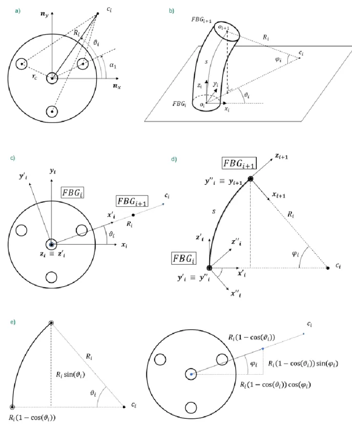
Fig. 1. Shape reconstruction algorithm based on homogenous transformation matrices. a) 𝐹𝐵𝐺𝑖 section view, {𝑛𝑥, 𝑛𝑦} plane - the information from
the outer cores allow for the calculation of the curvature vector of the overall fiber. The angle 𝛼𝑖 (𝑖 = 1,2,3) locates the position of the cores with
respect to versor 𝑛𝑥. b) From 𝐹𝐵𝐺𝑖 to 𝐹𝐵𝐺𝑖+1 - location 𝑜𝑖+1 is identified starting from 𝑜𝑖 with the knowledge of 𝜗𝑖, 𝑅𝑖 and triplet {𝑥𝑖, 𝑦𝑖, 𝑧𝑖}. c) 𝐹𝐵𝐺𝑖
section view, {𝑥𝑖, 𝑦𝑖} plane - 𝐹𝐵𝐺𝑖 senses a curvature radius 𝑅𝑖 and an azimuth angle 𝜗𝑖, which identify an in-plane rotation center 𝑐𝑖. 𝐹𝐵𝐺𝑖+1 is out
of the considered section plane. The first passage consists in aligning the x axis with the rotation center 𝑐𝑖.d) Multicore fiber, external side view,
{𝑥𝑖′, 𝑧𝑖′} plane - 𝐹𝐵𝐺𝑖+1 is located by performing a circular motion of length s (FBG distance) around center 𝑐𝑖 starting from 𝐹𝐵𝐺𝑖. The angle 𝜑𝑖 is
obtained from the known parameters 𝑅𝑖 and 𝑠, and is used to re-align the x axis towards the rotation center 𝑐𝑖.e) From 𝐹𝐵𝐺𝑖 to 𝐹𝐵𝐺𝑖+1 - location
B. Homogeneous transformation matrices
The shape-reconstructing method utilizes homogenous transformation matrices, useful to express the coordinates of a point in a different frame, as described in (3):
𝒑̃𝑖+1𝑖 = [ 𝑝𝑖+1,𝑥𝑖 𝑝𝑖+1,𝑦𝑖 𝑝𝑖+1,𝑧𝑖 1 ] = 𝑨𝑖+1𝑖 𝒑̃𝑖+1𝑖+1= [ 𝑹𝑖+1𝑖 𝒐𝑖+1𝑖 𝟎3𝑇 1 ] 𝒑̃𝑖+1𝑖+1 (3)
where 𝒑̃𝑖+1𝑖 are the homogeneous coordinates of 𝐹𝐵𝐺𝑖+1 with respect to the reference frame located at 𝐹𝐵𝐺𝑖, 𝑝𝑖+1,𝑘𝑖 with 𝑘 = {𝑥, 𝑦, 𝑧} is the 𝑘𝑡ℎ component of position 𝒑̃𝑖+1𝑖 𝑨𝑖+1𝑖 is the homogeneous transformation matrix from frame 𝑖 + 1 to frame 𝑖 and 𝒑̃𝑖+1𝑖+1 are the homogeneous coordinates of 𝐹𝐵𝐺𝑖+1 with respect to the reference frame located at 𝐹𝐵𝐺𝑖+1 itself, which correspond to the origin [0 0 0 1]𝑇. Homogenous transformation matrices always exhibit the same inner structure: 𝑹𝑖+1𝑖 is a 3x3 rotation matrix that aligns the orientation of the two considered frames, 𝒐𝑖+1𝑖 is the origin of frame 𝑖 + 1 expressed in frame 𝑖 and 𝟎3𝑇 is a 1x3 null vector. This change of coordinates will be adopted during the shape reconstruction to express all the FBG positions in the starting frame, with the aid of the property reported in the following equation:
𝒑̃𝑖+10 = 𝑨10𝑨21⋯ 𝑨𝑖𝑖−1𝑨𝑖+1𝑖 𝒑̃𝑖+1𝑖+1= 𝑨𝑖+10 𝒑̃𝑖+1𝑖+1 (4)
It is hereafter considered a cross-section of the fiber located at the 𝑖𝑡ℎ FBG location (Fig. 1b). The frame, represented by the unitary triplet {𝒙𝑖, 𝒚𝑖, 𝒛𝑖}, is rotated around 𝒛𝑖 of an angle 𝜗𝑖 (Fig. 1c) and around 𝒚𝑖′ of an angle 𝜑𝑖 (Fig. 1d).
The corresponding rotation matrices used to align the 𝑖-th frame with the (𝑖+1)-th frame are reported in (5) and (6).
𝑹𝒛𝒊(𝜗𝑖) = [ cos(𝜗𝑖) − sin(𝜗𝑖) 0 sin(𝜗𝑖) cos(𝜗𝑖) 0 0 0 1 ] (5) 𝑹𝒚 𝒊 ′(𝜑𝑖) = [ cos(𝜑𝑖) 0 sin(𝜑𝑖) 0 1 0 − sin(𝜑𝑖) 0 cos(𝜑𝑖) ] (6)
The origin of frame 𝑖+1 with respect to frame 𝑖 is obtained with the following trigonometric formula, as it is clearly shown in Fig. 1e: 𝒐𝑖+1𝑖 = [ 𝑅𝑖(1 − cos(𝜑𝑖)) cos(𝜗𝑖) 𝑅𝑖(1 − cos(𝜑𝑖)) sin(𝜗𝑖) 𝑅𝑖sin(𝜑𝑖) ] (7)
Equation (3) can be rewritten by including the information from (5), (6) and (7):
𝒑̃𝑖+1𝑖 = 𝑨𝑖+1𝑖 𝒑̃𝑖+1𝑖+1= [
𝑹𝒛𝒊(𝜗𝑖) 𝑹𝒚𝒊′(𝜑𝑖) 𝒐𝑖+1𝑖
𝟎3𝑇 1
] 𝒑̃𝑖+1𝑖+1 (8)
The complete inner structure of the homogenous transformation matrix is the following:
𝑨𝑖+1𝑖 = [ 𝑐𝑜𝑠(𝜗𝑖) 𝑐𝑜𝑠(𝜑𝑖) − 𝑠𝑖𝑛(𝜗𝑖) 𝑠𝑖𝑛(𝜗𝑖) 𝑐𝑜𝑠(𝜑𝑖) 𝑐𝑜𝑠(𝜗𝑖) − 𝑠𝑖𝑛(𝜑𝑖) 0 0 0 𝑐𝑜𝑠(𝜗𝑖) 𝑠𝑖𝑛(𝜑𝑖) 𝑅𝑖(1 − cos(𝜑𝑖)) cos(𝜗𝑖) 𝑠𝑖𝑛(𝜗𝑖) 𝑠𝑖𝑛(𝜑𝑖) 𝑅𝑖(1 − cos(𝜑𝑖)) sin(𝜗𝑖) 𝑐𝑜𝑠(𝜑𝑖) 𝑅𝑖sin(𝜑𝑖) 0 1 ] (9)
An approximation is introduced in this method: the curvature radius 𝑅𝑖 is assumed to be constant along the considered arc, whereas Fig. 2 shows that at location 𝑖+1 the actual value is 𝑅𝑖+1 Despite that, when the distance between two locations is small enough, the difference between 𝑅𝑖 and 𝑅𝑖+1 becomes negligible. An approach useful to reduce the potential error deriving from this approximation is based on the interpolation of the measured data on a larger number of virtual points along the length of the fiber, simulating a distributed FBG-based fiber.
C. Frenet-Serret equations
The same result achieved with Frenet-Serret can be obtained with the proposed algorithm, but with less virtual sensors (related to the interpolation factor m), as it will be shown in Section IV. As a reference for further discussion, the standard Frenet-Serret equations are reported below for clarity [24]:
𝑵(𝑖) =𝑠𝜏(𝑖)𝑩(𝑖 − 1) − 𝑠𝜅(𝑖)𝑻(𝑖 − 1) + 𝑵(𝑖 − 1) 1 + 𝑠2𝜏2(𝑖) + 𝑠2𝜅2(𝑖)
𝑻(𝑖) = 𝑠𝜅(𝑖)𝑵(𝑖) + 𝑻(𝑖 − 1) Fig. 2. External view of the fiber. While the change of curvature is
continuous along the length of the fiber, the information is available only at discrete points (FBG locations). The values of curvature between two contiguous FBGs are obtained with data interpolation.
𝑩(𝑖) = −𝑠𝜏(𝑖)𝑵(𝑖) + 𝑩(𝑖 − 1) (10) 𝒓(𝑖) = 𝑠𝑻(𝑖) + 𝒓(𝑖 − 1)
where 𝑖 is an integer representing the discrete location of the curve we are considering, corresponding to distance 𝑠 ∗ 𝑖 from the beginning, s represents the distance between two consecutive FBGs (which are virtual if data interpolation was performed) , 𝒓(𝑖) is the vector of the positions corresponding to the i-th FBG. {T(i),N(i),B(i)} is a triplet of orthogonal unitary vectors defined as the tangent (T), normal (N) and binormal (B) vectors to the curve, abbreviated as TNB triplet.
The Frenet-Serret equations reported in (10) belong to the discrete domain and are presented in a form that can be accepted by a software that executes operations in a sequential order (i.e. MATLAB).
The scalar functions 𝜏(𝑖) and 𝜅(𝑖) are the torsion and the curvature of the shape; function 𝜅(𝑖) is the same reported in (2) whereas the torsion function is defined as:
𝜏(𝑖) = (𝜗(𝑖) − 𝜗(𝑖 − 1))/𝑠 (11)
The Frenet-Serret equations assume 𝑠 to be infinitesimal and the curve to always be well defined (curvature radius 𝑅 < ∞) so that the triplet TNB can be univocally defined. An infinitesimal s can be achieved with a sufficiently large interpolation factor m, which creates a wider set of virtual FBGs with shorter distance between each other. On the other hand, because the fiber can be straight in certain points or segments, a curvature cannot be always guaranteed. Nonetheless, some techniques or variations can be implemented to prevent this situation (e.g., parallel transport [27], negative curvature [28]).
III. MULTICORE FIBER AND EXPERIMENTAL SETUP In order to evaluate the performance of the above-described algorithms, 3D FBG arrays contained in a polyimide-coated 7-core optical fiber manufactured by the Fiber Optics Research Center (Moscow, Russia) were used. The fiber has seven identical straight cores – the central one and six surrounding side cores located in the corners of a regular hexagon. The distance between the cores is 40.5 μm, the cladding diameter is 125 μm, and the mode field diameter for each core is 5.7 μm at 1550 nm. The fiber is coated with a 15 μm thick polyimide layer, thus giving the outer fiber diameter of 154 μm. To couple
optical signals into separate cores, a matching fan-out device was used. The polyimide protective coating of the fiber provides the high mechanical strength and the high-temperature resistance (short term up to 400 °C and continuous operation at 300 °C) in comparison with acrylate one (up to 85 °C) [23,29]. These properties make this sensor well-suited for harsh environments or for some medical and composite material applications.
To fabricate an FBG array the femtosecond plane-by-plane method was used, which is based on focusing an astigmatic femtosecond beam in the region of a fiber core [15]. In the case under study the infrared femtosecond pulses are produced by Light Conversion Pharos 6W laser (wavelength 𝜆 = 1030 nm, pulse duration 𝑡𝑝 = 232 fs, and pulse repetition rate 𝑓 = 1 kHz). In order to focus femtosecond pulses into the fiber it was used a Mitutoyo 50X Plan Apo NIR HR objective (NA = 0.65) and an additional cylindrical lens with a focal distance 𝑓𝑐 = −1000 mm, mounted before the objective. A special glass ferrule with polished side faces makes it possible to fix the transverse position of the multicore fiber with respect to the focal point [30]. The longitudinal periodic modulation of the refractive index is achieved by moving the fiber with a predefined constant velocity 𝜈𝑡𝑟 ≈ 1 mm/s (2nd order of Bragg resonance), by using an Aerotech ABL1000 high-precision air-bearing linear stage. Thus, the FBG period is determined by Λ = 𝜈𝑡𝑟/𝑓, and the resonant wavelength by 𝜆𝐵= 2𝑛𝑒𝑓𝑓𝜈𝑡𝑟/(𝑚𝑓), where 𝑚 = 2 is the order in which resonant reflection of the optical signal on the FBG structure is realized. The end of the fiber, threaded through the ferrule, is fixed on the linear stage with the help of a clamp with an angular degree of freedom allowing to turn the fiber around its axis. Inscription of FBGs in the multicore fiber was carried out through the polyimide coating. Two different multicore fibers were used in the experiments in order to show the independency of the algorithm properties from the specific fiber under test.
The first one (fiber #1) consists of 6 nodes along the fiber with an interval between the centers of the adjacent nodes
Fig. 3. Multicore fiber. Schematic representation of a 3D FBG array inscribed in the polyimide-coated 7-core optical fiber: a) 3D view and
ΔL1 = 14 mm, and the second one (fiber #2) consists of 9 nodes
along the fiber with an interval between the centers of the adjacent nodes ΔL2 = 10 mm. In each node, uniform FBGs with
a constant length LFBG = 2 mm were inscribed in the central
core, and in three side cores located at the corners of an equilateral triangle. Thereby the total length of fiber #1 was L1
= 72 mm, and the total length of fiber #2 was L2 = 82 mm. A
schematic representation of the created fibers, as well as the FBG numbering in the arrays, is shown in Fig. 3. Uniform distribution of FBG resonant wavelengths along the same core is ensured by sequential variation of FBG periods.
To interrogate the fabricated multicore fibers, the HBM FS22-SI 8-channel interrogation unit (wavelength range from 1500 nm to 1600 nm, Fig. 4) was used. The processing of the measured spectra, detection and tracking of the FBG reflection peaks, was maintained with the BraggMONITOR SI application. More information about the procedure of the shape sensor calibration and relevant data can be found in [15].
When reconstructing the fiber shape, different curves were analysed, including different 2D bow-like and s-like curves, and a 3D spiral wound onto a surface of cylinder. In order to diminish possible torsions, the straight section of the fiber containing an FBG array was glued with adhesive tape and then taped to a sheet of scale paper in the desired shape. To get the ground truth data, a photo of a fiber laying on a paper was taken and the shape digitized with a specialized software tool. The 3D spiral had a diameter D = 25 mm and pitch h = 10 mm. The winding of the fiber was done under tension to ensure a snug fit and by following the reference line drawn onto a cylinder surface, whereas the ends of the sensor were sealed with adhesive tape. In this case, as a ground truth data we used the curve obtained from analytical formulas for a 3D spiral.
IV. RESULTS AND DISCUSSION
The shape reconstruction is shown for three different setups, namely a spiral, a bow and an S shape. A previous analysis for similar spiral shapes can be found in [15]. The structure chosen for presenting the results is the following:
1) The reconstruction is iterated for both methods for a large number of increasing values of the interpolation factor m, and the average error, i.e. the mean of the Euclidean distances between the reconstructed points and the ground truth, is plotted. By fixing a value for the interpolation factor m it is possible to compare the accuracy of the two algorithms. By choosing a value for the average error it is possible to understand which is the interpolation factor m that is required for the algorithms to provide such result.
2) After selecting a value for the interpolation factor m, the shape reconstruction is graphically presented. The figure presents a clear view of the results that can be achieved in the two cases.
3) The evolution of the curvature modulus and phase is shown so that it is possible to analyse the properties of the shape, such as inflection points, where the modulus tends to zero and the phase exhibits a shift of 180°. 4) The evolution of the norm of the three orthonormal
versors calculated with the Frenet-Serret equations, i.e., T N and B, is reported. The reconstruction is hindered if the norm of these vectors strays from the unitary value, which is very evident in the case of inflection points in the shapes under study.
5) Lastly, a table reports the relevant data of the experiment, such as the calculated strains and the accuracy and performance of the algorithms. The performance is evaluated, with the MATLAB tic toc function, in terms of average computation time over 1000 instances of the algorithms, and the average refresh rate (calculated as the inverse of the average computation time) gives an idea of the possible reconstruction capabilities in a real-time application. The algorithms were executed sequentially, no multi-thread was applied.
The relevant specifications of the terminal used for the performance analysis are the following: Processor: Intel(R) Core (TM) i7-8565U CPU @ 1.80GHz, 1992 MHz, 4 Core(s), 8 Logical Processor(s), RAM: 8 GB.
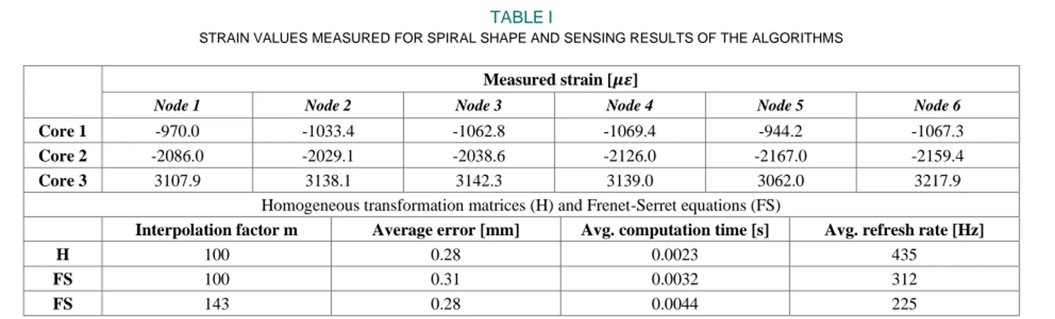
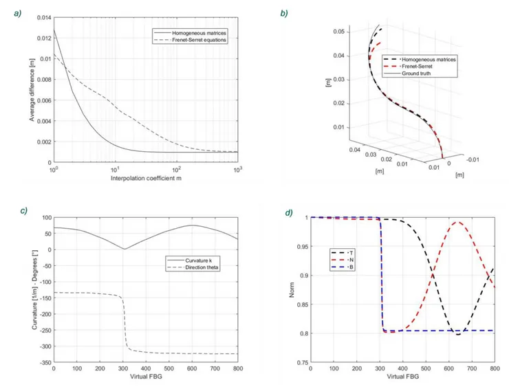
Results for the spiral shape with the multicore 6 FBG fiber are reported in Fig. 5 and Table 1. The reconstruction is highly accurate since the obtained average errors are sub millimetric, and both algorithms are viable for applications like the medical ones (catheters, flexible endoscopes), where the precision in the reconstructed shape is paramount for a successful procedure [20]. The interpolation factor chosen in Fig. 5b is 𝑚 = 100; it is the smallest value that minimizes the reconstruction error, and corresponds to 100 segments with a length of 0.14 mm between two consecutive FBGs. The best achievable average error is 0.28 mm; as shown in Fig. 5c, the curvature is not perfectly constant, nor the direction angle is perfectly linear. The evolution of the norms of the TNB triplet is shown in Fig. 5d; although not being unitary, the difference is small enough and the shape can be properly reconstructed with the Frenet-Serret equations. The average error obtained for the spiral shape is comparable with the results obtained in a previous work for similar 3D shapes and sizes, which reports a mean error ranging from 0.12 mm to 0.23 mm [21].
Results for the bow shape with the multicore 6 FBG fiber are reported in Fig. 6 and Table 2. The presence of two inflection points in the curve (Fig. 6c) causes the TNB triplet to noticeably lose the unitary norm (Fig. 6d) and compromises the reconstruction (Fig. 6b). The interpolation factor chosen for the reconstruction is 𝑚 = 100, in accordance with the choice made in the spiral experiment (and corresponding to 100 segments 0.14 mm-long between two successive FBGs centers). The best achievable average error is 0.39 mm. For very large interpolation factors m, the discontinuity in phase is divided in shorter intervals where the difference between two sequential values of the angle becomes acceptable and the Frenet-Serret reconstruction recovers accuracy. As it can be seen in Fig. 6a, the reconstruction error for Frenet-Serret tends to the same value of the transformation matrices for increasing values of interpolation. In fact, the perturbation of the Frenet-Serret frame shown in Fig. 6d, although maintaining its shape, will be scaled down and become negligible. The downside is obviously the computational effort needed to perform the satisfactory level of interpolation on the data. On the other hand, the proposed algorithm is insensitive to discontinuities in the phase and performs well even at low values of interpolation.
Results for the s-shape with the multicore 9 FBG fiber are reported in Fig. 7, as well as in Table 3. The difference in accuracy is noticeable, proving that even a single inflection point in the shape hinders the traditional Frenet-Serret
reconstruction. As already stated for the previous experiment, a large effort in interpolation can mitigate the intensity of the perturbation and yield results close to the ones obtained with the homogeneous transformation matrices, at the cost of the computational performance. The interpolation factor chosen for the reconstruction is 𝑚 = 100. In this case, being the distance between nodes equal to 10 mm, the choice of m corresponds to 100 segments (length of each segment is 0.1 mm) between two consecutive FBGs. The best achievable average error with this interpolation factor is 1.00 mm. This last result is comparable with previous data provided in [20], where a average error of 1.15 mm is obtained on a 38 cm catheter, after implementing curvature and angle correction.
The results of the experiments show that the accuracy of the overall sensing system depends on three main factors: the reconstruction algorithm, the multicore fiber under test and the complexity of the forms. Once a fiber is selected, and a desired average reconstruction error threshold is fixed, the choice of the algorithm determines the performance in terms of execution time. The algorithm based on transformation matrices scores better than the traditional Frenet-Serret equations in all the presented cases.
Another important result is that the method based on transformation matrices, with the available hardware, can run at an average frequency of 435 Hz for the 6 FBG array (spiral, bow) and 324 Hz for the 9 FBG array (s-shape). The Frenet-Serret algorithm, executed with an interpolation factor that allows reaching the same average error obtained with the transformation matrices, scores an average frequency of 225 Hz (spiral, 6 FBG array), 6 Hz (bow, 6 FBG array) and 20 Hz (s-shape, 9 FBG array).
Frenet-Serret equations have been largely investigated as a method for shape reconstruction, and recently compared to other approaches and improved versions, such as Bishop frame [20,31]. Among the alternative approaches, transformation matrices have demonstrated good performances for 3D shape sensing. A kinematics-based model based on homogeneous transformation was introduced and assessed also in [32], aimed at calculating the deflection of a needle embedding three separated optical fibers. In accordance with the preliminary reports by [20,22], the method based on transformation matrices has shown better performances than Frenet-Serret equations in 3D shape sensing performed also with the proposed multicore fiber. The present work further investigates the influence of parameters of the algorithms on the performances of the two methods for the shape reconstruction; the results are given for every choice of the interpolation factor and the selected shapes are characterized by high curvatures, while the aforementioned work only focuses on shapes with mild curvatures and for a single choice of parameters. A detailed comparison with the state of the art in terms of both evolution of the accuracy depending on the interpolation factor and computational efforts is given in the present work. Furthermore, the results are shown for two different custom-made multicore fibers in order to prove the uncorrelation between the algorithm properties and the specific fiber under test.
TABLEI
STRAIN VALUES MEASURED FOR SPIRAL SHAPE AND SENSING RESULTS OF THE ALGORITHMS
Measured strain [𝝁𝜺]
Node 1 Node 2 Node 3 Node 4 Node 5 Node 6
Core 1 -970.0 -1033.4 -1062.8 -1069.4 -944.2 -1067.3
Core 2 -2086.0 -2029.1 -2038.6 -2126.0 -2167.0 -2159.4
Core 3 3107.9 3138.1 3142.3 3139.0 3062.0 3217.9
Homogeneous transformation matrices (H) and Frenet-Serret equations (FS)
Interpolation factor m Average error [mm] Avg. computation time [s] Avg. refresh rate [Hz]
H 100 0.28 0.0023 435
FS 100 0.31 0.0032 312
FS 143 0.28 0.0044 225
Fig. 5. Spiral – 3D. a) Spiral reconstruction, average error - the average distance between the points calculated by the two different algorithms with the same interpolation factor and the ground truth is presented. As the interpolation factor is increased, the difference becomes negligible. b) 3D spiral reconstruction - ground truth (solid line), recovered shape with the proposed method (dashed black line) and recovered shape with Frenet-Serret (dashed red line) are shown. The chosen interpolation factor is m=100 as it provides a trade-off between accuracy and performance. c) Spiral curvature and direction angle - the measured curvature [𝑚−1] (solid line) and the measured
curvature direction [°] (dashed line) are presented. The almost constant curvature is in accordance with the constant radius of the cylinder and the behavior of the direction angle 𝜃 is similar to the linear one of a spiral pitch. d) Norms of the Frenet-Serret versors (spiral) - the evolution of the norms of the TNB triplet is presented. Although not being unitary, the norm is preserved enough to yield a good result. By increasing the interpolation factor m, the decadence maintains its shape but is decreased in amplitude, in accordance with Fig. 5a.
c)
b) a)
Fig. 6. Bow – 2D. a) Bow reconstruction, average error - the average distance between the points calculated by the two different algorithms with the same interpolation factor and the ground truth is presented. Although the difference becomes negligible as the interpolation factor is increased, it is noticeable for all interpolation factors m<5000. b) 3D bow reconstruction - ground truth (solid line), recovered shape with the proposed method (dashed black line) and recovered shape with Frenet-Serret (dashed red line) are shown. The chosen interpolation factor is m=100 to be consistent with the choice previously made for the spiral. c) Bow curvature and direction angle - the measured curvature [𝑚−1] (solid line) and the measured curvature direction [°] (dashed line) are presented. The evolution of the curvature direction
reflects the double bend of the shape. d) Norms of the Frenet-Serret versors (bow) - the evolution of the norms of the TNB triplet is presented. The double change in direction affects the norm of the TNB triplet, but the algorithm still manages to yield acceptable results for very large interpolation factors, where the norm drop is mitigated in amplitude.
TABLEII
STRAIN VALUES MEASURED FOR THE BOW SHAPE AND SENSING RESULTS OF THE ALGORITHMS
Measured strain [𝝁𝜺]
Node 1 Node 2 Node 3 Node 4 Node 5 Node 6
Core 1 -831.9 711.9 1943.0 2004.2 797.2 -583.9
Core 2 571.7 -386.2 -834.2 -607.4 -156.9 -58.0
Core 3 324.5 -234.0 -1080.9 -1352.7 -678.1 623.8
Homogeneous transformation matrices (H) and Frenet-Serret equations (FS)
Interpolation factor m Average error [mm] Avg. computation time [s] Avg. refresh rate [Hz]
H 100 0.39 0.0023 435
FS 100 2.70 0.0032 312
Fig. 7. S-shape – 2D. a) S-shape reconstruction, average error - the average distance between the points calculated by the two different algorithms with the same interpolation factor and the ground truth is presented. For increasing interpolation factors m, the error decreases and the Frenet-Serret reconstruction reaches the same output of the presented algorithm. b) 3D s-shape reconstruction - ground truth (solid line), recovered shape with the proposed method (dashed black line) and recovered shape with Frenet-Serret (dashed red line) are shown. The chosen interpolation factor is m=100 to be consistent with the choice previously made for the spiral. c) S-shape curvature and direction angle - the measured curvature [𝑚−1] (solid line) and the measured curvature direction in degrees (dashed line) are presented.
The direction angle has been a posteriori modified to prevent arctangent discontinuities from occurring. d) Norms of the Frenet-Serret versors (s-shape) - the evolution of the norms of the TNB triplet is presented.
TABLEIII
STRAIN VALUES MEASURED FOR THE S-SHAPE AND SENSING RESULTS OF THE ALGORITHMS
Measured strain [𝝁𝜺]
Node 1 Node 2 Node 3 Node 4 Node 5 Node 6 Node 7 Node 8 Node 9
Core 1 1818.1 1458.1 711.4 2.3 -406.7 -421.2 -178.4 139.6 181.8
Core 2 475.0 745.0 678.3 101.6 -886.0 -1943.8 -2690.5 -2332.5 -1270.6
Core 3 -2771.6 -2555.1 -1557.0 -82.3 1212.6 2143.2 2547.5 1896.4 855.3
Homogeneous transformation matrices (H) and Frenet-Serret equations (FS)
Interpolation factor m Average error [mm] Avg. computation time [s] Avg. refresh rate [Hz]
H 100 1.00 0.0031 324
FS 100 1.65 0.0050 201
V. CONCLUSION
This work presents a comparison between two different three-dimensional reconstruction algorithms for the estimation of the shape of a multicore fiber optic-based sensing system. The designed multicore fibers allow an accurate measurement of their shape, which makes them suitable for those applications where accuracy is paramount. A non-exhaustive list of potential fields of interest for the application is: medical and industrial robotics, mining industry and aerospace. The algorithm based on transformation matrices is characterized by a better performance in respect to the traditional Frenet-Serret equations, proving to be suitable for applications where fast real-time feedback is needed; in fact, it is able to provide the same accuracy with lower computational effort, while also being more stable against discontinuities in the measured curvature angle values. Future works will involve developing a real-time application of the algorithm.
REFERENCES
1. Amanzadeh, M., Aminossadati, S.M., Kizil, M.S., and Rakić, A.D. (2018) Recent developments in fibre optic shape sensing.
Measurement, 128, 119–137.
2. Elayaperumal, S., Park, Y., Savall, J., Cutkosky, M.R., Daniel, B., Shin, M., Moslehi, B., Black, R.J., and Ryu, S.C. (2010) Real-Time Estimation of 3-D Needle Shape and Deflection for MRI-Guided Interventions. IEEE/ASME Trans. Mechatronics, 15 (6), 906–915. 3. Boctor, E.M., Choti, M.A., Burdette, E.C., and Webster Iii, R.J.
(2008) Three‐dimensional ultrasound‐guided robotic needle placement: an experimental evaluation. Int. J. Med. Robot. Comput.
Assist. Surg., 4 (2), 180–191.
4. Su, X., and Zhang, Q. (2010) Dynamic 3-D shape measurement method: a review. Opt. Lasers Eng., 48 (2), 191–204.
5. Zhang, S. (2010) Recent progresses on real-time 3D shape measurement using digital fringe projection techniques. Opt. Lasers
Eng., 48 (2), 149–158.
6. Ohno, K., Nomura, T., and Tadokoro, S. (2006) Real-time robot trajectory estimation and 3d map construction using 3d camera. 2006
IEEE/RSJ Int. Conf. Intell. Robot. Syst., 5279–5285.
7. Peña, F., Richards, L., Parker Jr, A.R., Piazza, A., Chan, P., and Hamory, P. (2015) Fiber Optic Sensing System (FOSS) technology-A new sensor paradigm for comprehensive structural monitoring and model validation throughout the vehicle life-cycle.
8. Danisch, L., Chrzanowski, A., Bond, J., and Bazanowski, M. (2008) Fusion of geodetic and MEMS sensors for integrated monitoring and analysis of deformations. 13th FIG Int. Symp. Deform. Meas. Anal.
Lisbon, Port. May, 12–15.
9. Dementyev, A., Kao, H.-L.C., and Paradiso, J.A. (2015) Sensortape: Modular and programmable 3d-aware dense sensor network on a tape. Proc. 28th Annu. ACM Symp. User Interface Softw. Technol., 649–658.
10. Kersey, A.D., Davis, M.A., Patrick, H.J., LeBlanc, M., Koo, K.P., Askins, C.G., Putnam, M.A., and Friebele, E.J. (1997) Fiber grating sensors. J. Light. Technol., 15 (8), 1442–1462.
11. Udd, E., and Spillman Jr, W.B. (2011) Fiber optic sensors: an
introduction for engineers and scientists, John Wiley & Sons.
12. Othonos, A., Kalli, K., and Kohnke, G.E. (2000) Fiber Bragg gratings: Fundamentals and applications in telecommunications and sensing. Phys. Today, 53 (5), 61.
13. Froggatt, M.E., and Duncan, R.G. (2010) Fiber optic position and/or
shape sensing based on Rayleigh scatter.
14. Froggatt, M.E., Klein, J.W., Gifford, D.K., and Kreger, S.T. (2014) Optical position and/or shape sensing.
15. Bronnikov, K., Wolf, A., Yakushin, S., Dostovalov, A., Egorova, O., Zhuravlev, S., Semjonov, S., Wabnitz, S., and Babin, S. (2019) Durable shape sensor based on FBG array inscribed in polyimide-coated multicore optical fiber. Opt. Express, 27 (26), 38421–38434. 16. Froggatt, M., and Moore, J. (1998) High-spatial-resolution
distributed strain measurement in optical fiber with Rayleigh scatter.
Appl. Opt., 37 (10), 1735–1740.
17. Masoudi, A., and Newson, T.P. (2016) Contributed Review: Distributed optical fibre dynamic strain sensing. Rev. Sci. Instrum., 87 (1), 11501.
18. Erdogan, T. (1997) Fiber grating spectra. J. Light. Technol., 15 (8), 1277–1294.
19. Lee, K.K.C., Mariampillai, A., Haque, M., Standish, B.A., Yang, V.X.D., and Herman, P.R. (2013) Temperature-compensated fiber-optic 3D shape sensor based on femtosecond laser direct-written Bragg grating waveguides. Opt. Express, 21 (20), 24076–24086. 20. Jäckle, S., Eixmann, T., Schulz-Hildebrandt, H., Hüttmann, G., and
Pätz, T. (2019) Fiber optical shape sensing of flexible instruments for endovascular navigation. Int. J. Comput. Assist. Radiol. Surg. 21. Khan, F., Denasi, A., Barrera, D., Madrigal, J., Sales, S., and Misra,
S. (2019) Multi-Core Optical Fibers with Bragg Gratings as Shape Sensor for Flexible Medical Instruments. IEEE Sens. J.
22. Chen, X., Yi, X., Qian, J., Zhang, Y., Shen, L., and Wei, Y. (2020) Updated shape sensing algorithm for space curves with FBG sensors.
Opt. Lasers Eng., 129, 106057.
23. Dostovalov, A. V, Wolf, A.A., Parygin, A. V, Zyubin, V.E., and Babin, S.A. (2016) Femtosecond point-by-point inscription of Bragg gratings by drawing a coated fiber through ferrule. Opt. Express, 24 (15), 16232–16237.
24. Moore, J.P., and Rogge, M.D. (2012) Shape sensing using multi-core fiber optic cable and parametric curve solutions. Opt. Express, 20 (3), 2967–2973.
25. Rabbath, C.A., and Corriveau, D. (2019) A comparison of piecewise cubic Hermite interpolating polynomials, cubic splines and piecewise linear functions for the approximation of projectile aerodynamics.
Def. Technol.
26. Esfandiari, R.S. (2017) Numerical methods for engineers and
scientists using MATLAB®, second edition.
27. Cui, J., Zhao, S., Yang, C., and Tan, J. (2018) Parallel transport frame for fiber shape sensing. IEEE Photonics J.
28. Moore, J.P. (2010) Method and apparatus for shape and end position determination using an optical fiber.
29. Gratten, K.T. V, and Meggitt, B.T. (1999) Optical Fiber Sensor
Technology: Volume 3: Applications and Systems, Kluwer Academic
Pub.
30. Wolf, A., Dostovalov, A., Bronnikov, K., and Babin, S. (2019) Arrays of fiber Bragg gratings selectively inscribed in different cores of 7-core spun optical fiber by IR femtosecond laser pulses. Opt.
Express, 27 (10), 13978–13990.
31. Khan, F., Donder, A., Galvan, S., Baena, F.R. y, and Misra, S. (2020) Pose Measurement of Flexible Medical Instruments using Fiber Bragg Gratings in Multi-Core Fiber. IEEE Sens. J.
32. Roesthuis, R.J., Kemp, M., Van Den Dobbelsteen, J.J., and Misra, S. (2014) Three-dimensional needle shape reconstruction using an array of fiber bragg grating sensors. IEEE/ASME Trans. Mechatronics.
Davide Paloschi(M’20) received the B.S. and M.S. degrees in automation and control engineering from Politecnico di Milano, Milan, Italy in 2016 and 2018, respectively.
From 2019, he is a Research Fellow at Politecnico di Milano in the department of mechanical engineering. He is currently involved in the LASER OPTIMAL@POLIMI project for the designing and prototyping of a wearable system for posture monitoring. As a Research Fellow, his main research interests regard the 3D reconstruction of the shape of optical fibers. His other research interests are model prediction, data analysis, noise filtering and machine learning.
Kirill A. Bronnikov received the B.S. degree in physics from Novosibirsk State University, Novosibirsk, Russia, in 2016 and the M.S. degree in physics from joint program of Novosibirsk State University, Novosibirsk, and Skolkovo Institute of Science and Technology, Moscow, Russia, in 2018. He is currently pursuing the Ph.D. degree in physics and astronomy at Novosibirsk State University.
Since 2016 he has been a Research Engineer with the Institute of Automation and Electrometry of the Siberian Branch of the Russian Academy of Sciences, Novosibirsk, Russia. His research interests include fiber optic sensors, femtosecond laser material processing and structuring, plasmonics, optical properties of metal-dielectric structures and metamaterials.
Sanzhar Korganbayev (M’20) received the B.S. and M.S. degrees in Electrical and Electronic Engineering from Nazarbayev University, Nur-Sultan, Kazakhstan in 2016 and 2018, respectively.
Currently, he is a Ph.D. student at the Department of Mechanical Engineering, Politecnico di Milano. He is currently involved in the the "LASER OPTIMAL” project (European Research Council grant GA 759159) for the he development of software for real-time temperature monitoring and intra-operative adjustment of the laser ablation settings during tumor treatment. His research interests include fiber optic sensors and their applications for thermal and mechanical measurements.
Alexey Wolf received the B.S. and M.S. degrees in physics with specialization in quantum optics from Novosibirsk State University (Novosibirsk, Russia) in 2011 and 2013, respectively. In 2017 he completed the Ph.D. program in optics in the Institute of Automation and Electrometry of the SB RAS (Novosibirsk, Russia). He is preparing to defend a dissertation on the technology of fabrication of advanced fiber Bragg gratings with femtosecond laser pulses. His research interests include femtosecond laser micromachining technology and development of novel fiber-optic devices.
Alexander Dostovalov received the B.S. and M.S. degrees in physics from the Novosibirsk State University in 2009 and the Ph.D. degree in optics from Institute of Automation and Electrometry of the Siberian Branch of the Russian Academy of Sciences, Novosibirsk, in 2015. From 2012 to 2016, he was a junior research fellow with Institute of Automation and Electrometry. From 2016 to 2018, he was a research fellow with Institute of Automation and Electrometry. Since 2018, he has been a senior research fellow with Institute of Automation and Electrometry. He is the author of more than 30 articles and 4 inventions. His research interests include femtosecond laser micromachining, fiber Bragg gratings inscription, fiber lasers and sensors.
Paola Saccomandi(M’11-SM’20)received her PhD in Biomedical Engineering from Università Campus Bio-Medico di Roma in 2014. From 2016 to 2018 she was postdoctoral researcher at the IHU - Institute of Image-Guided Surgery of Strasbourg. Since 2018 she is Associate Professor at the Department of Mechanical Engineering of Politecnico di Milano. She is the Principal Investigator of the European Research Council grant "LASER OPTIMAL”- GA 759159. The main research interests of Prof. Saccomandi and her team include fiber optic sensors, mechanical and thermal measurements, biomedical imaging, and the development of light-based approaches for hyperthermal tumor treatment and monitoring.