Characterization of the co-seismic slip field for large earthquakes

(1)

Alma Mater Studiorum · Universit`

a di Bologna

FACOLT `A DI SCIENZE MATEMATICHE, FISICHE E NATURALI

Corso di Laurea Magistrale in Fisica del Sistema Terra

Characterization of the co-seismic slip field

for large earthquakes

Relatore:

Prof. Stefano Tinti

Correlatore:

Prof. Alberto Armigliato

Presentata da:

Enrico Baglione

Sessione autunnale

(2)

Abstract

Focused studies on large earthquakes have highlighted that ruptures on generating faults are strongly heterogeneous. The main aim of this thesis is to explore characteristic patterns of the slip distribution of large earthquakes, by using the finite-fault models (FFM) obtained in the last 25 years.

A result of this thesis is the computation of regression laws linking focal parameters with magnitude. Particular attention was devoted to the aspect ratio (A.R.), defined as the ratio between fault length and width. FFMs have been partitioned in 3 A.R. classes and for each class, the position of the hypocentre, of the maximum slip and their mutual relation were investigated.

To favour inter-comparison, normalised images of on-fault seismic slip were produced on geometries typical of each A.R. class with the goal of finding possible regularities of the slip distribution shapes. In this thesis, the shape of the single-asperity FFMs has been fitted by means of 2D Gaussian distributions. To the knowledge of the author, this thesis is the first example of a systematic study of finite-fault solutions to identify the main pattern of the on-fault co-seismic slip of large earthquakes.

One of the foreseen applications is related to tsunamigenesis. It is known that tsunamis are mainly determined by the vertical displacement of the seafloor induced by large submarine earthquakes. In this thesis, the near-source vertical-displacement fields produced by the FFM (assumed as the real one), by a homogeneous fault model, by a depth-heterogeneous fault model and by two distinct 2D Gaussian distribution fault models were computed and compared for all single-asperity earthquakes. The main finding is that 2D Gaussian distributions give the least misfit fields and are therefore the most adequate for tsunami generation modelling.

(3)

(4)

Introduction

Large earthquakes (i.e. earthquakes with significant values of magnitude, typically larger than 6) are known to have distribution of slip on the fault plane that is not homogeneous, though in several applications and contexts (for instance for modelling of earthquake-induced tsunamis) a uniform distribution is assumed as a reasonably good approximation. How the co-seismic slip distributes on the fault is the main topic of this thesis, and the data used for this study are mostly the finite-fault models (FFM) of the SRCMOD database that can be accessed online. These slip models were obtained by using different data sources (geodetic, strong motion, teleseismic, local P waves, inSAR, and, in the best cases, a combination of two or more of them), and different crustal models, and by different inversion techniques and stabilization methods, and different spatial sampling (Manighetti et al., 2005).

Regression laws between the geometrical properties of the fault and the magnitude are obtained and compared to some of the laws of previous studies and published in the literature. Among the studied parameters, the fault area and length result the ones showing the highest correlation with magnitude. The aspect ratio, that is the length to width ratio, has been also regressed against the earthquake magnitude, which is a novelty of this study never examined before: as will be described in detail later, we found that the aspect-ratio vs. magnitude correlation is good mainly for the strike-slip events. The aspect ratio has been used in the present work to create three classes of earthquakes or, which is equivalent in our context, of FFMs. The original FFM have been rescaled to the typical dimension of each class and the rescaled FFM have been analysed to investigate the position of the hypocentre with respect to the regions of significant slip (and of the maximum) slip. Thanks to the FFM representation, through a qualitative analysis, it is shown that the hypocentre rarely lies close to the fault centre or to the peak of slip, but that more often it is found at the margin of an asperity, that is a region of significantly high slip. This result agrees with that obtained by Mai et al. (2005), for whom hypocentres are located either within or close to regions of large slip. The number of asperities, furthermore, tend to increase with the increasing of the aspect ratio. For smaller magnitudes, the position of the slip peak is often close to the centre of the fault. Its distance from the fault centre tends to increase in parallel with the magnitude.

(7)

The generation of standardized images of the rescaled FFM allowed us to analyse the distribution of the slip and compare different models by means of properly introduced similarity indexes. The property of most FFM to exhibit a single and clear region of high slip (i.e. a single asperity) has suggested us to best-fit the slip model by means of a 2D Gaussian distribution. We have used two different methods (least-square and highest-similarity) for such fitting hence obtaining two distinct 2D Gaussian distributions for each FFM. Since the main interest of the line of research started with this thesis is the generation of tsunamis by earthquakes, we have calculated the vertical displacements induced by the earthquake at the Earth surface in the near field. We have computed such fields with the FFM slip (assumed to be the real one), with an equivalent uniform-slip model, with a depth-dependent slip model, and with the two “best” Gaussian slip models. Results show that using uniform slip sources one can get discrepancies in the surface fields larger than 50% on average, which is slightly reduced with depth-dependent sources. The best results are the ones obtained with 2D Gaussian distributions based on similarity index fitting.

The study of this thesis sets the basis for a following research project to be carried out by the author during the PhD work where the aim is to explore the feasibility of a real-time assessment of the co-seismic slip of large earthquakes having high tsunamigenic potential. And, among these, the shallow events with potential consequences in the near field will assume more importance, because the near field is known to be more susceptible to the heterogeneous distribution of the slip.

1.1 The on-fault slip distribution: an overview

The distribution of the slip over the fault has already been object of numerous studies, especially in the last decades, thanks to the source-inversion methods and the growth of the available amount of data.

Though it is out of the scope of this thesis to make a detailed, but painstaking, review of all the related literature, it is however worth mentioning some of the most relevant studies.

Beroza (1991), analysing data from the 1989 Loma Prieta earthquake, analyses the slip distribution by using a tomographic back-projection technique. He finds a correlation between areas of high slip and areas of low aftershock activity, explaining this by

(8)

stating areas of high slip are also areas of high strength, that rupture completely only during infrequent large mainshocks.

Mai and Beroza (2000) develop a stochastic characterization of earthquake slip complexity: they model the slip as a spatial random field, more precisely as a von Karman autocorrelation function (ACF) model, with parameters depending on the source dimension.

Milliner et al. (2016) find a spatial correlation between fluctuations of the slip distribution and geometrical fault structure. Studying the 1992 Landers and 1999 Hector Mine earthquakes, they discover that the spatial frequency content of the fault structure can be observed within the slip distribution, which is suggestive that rougher faults systems produce rougher co-seismic slip at all scales.

1.2 Source slip distribution and tsunami

Most tsunami models assume that the initial sea surface displacement is equal to the vertical displacement of the sea floor induced by the earthquake that is computed by means of standard analytical models based on Volterra’s theory of elastic dislocations. Further common assumption is that the slip over the fault plane is uniform. However, modern teleseismic and geodetic inversion techniques have confirmed that the assumption of a uniform slip over the entire rupture plane is invalid.

The way the slip is distributed has direct influence on the possible generated tsunami. Many numerical simulations have highlighted that the same scenarios show very different results depending on whether one considers or not a uniform slip model.

An example of these investigations is the work by Geist (2002), who studied the effect of rupture complexity on the local tsunami wave field. Geist noticed that in the far-field tsunami amplitudes are well predicted only on the basis of the seismic moment, but that this is not true for local tsunami amplitudes. Looking at a global catalogue of tsunami runup observations, he noticed that discrepancy is larger for the most frequently occurring tsunamigenic earthquakes in the magnitude range of 7 < Mw < 8.5, which is actually included in the range of interest for our study. Variability in local tsunami runup scaling can be ascribed to tsunami source parameters that are independent of seismic moment such as: variations in the sea depth in the source region, the combination of higher slip and lower shear modulus at shallow depth, and rupture

(9)

complexity in the form of heterogeneous slip distribution patterns. Geist showed that, for shallow subduction zone earthquakes, self-affine irregularities of the slip distribution result in significant variations in local tsunami amplitude and that the effects of rupture complexity are less pronounced for earthquakes at greater depth or along faults with steep dip angles.

The influence of fault parameters on the maximum runup has been, among others, pointed out by Løvholt et al. (2012). They analysed how heterogeneous coseismic slip affects the initial water surface elevation and consequently the tsunami runup on the coast for a high number of stochastic slip realizations. These different realizations result in a range of initial seabed responses. They explored the relevance on the simulated maximum runup of different parameters. Among them, the most important were shown to be the scaled seabed volume displaced per unit length and the maximum peak-to-peak vertical seabed displacement.

Relevance to this subject has also the abundant literature published on the two greatest and most destroying earthquakes of the last 25 years: i.e. the 26 December 2004 Sumatra–Andaman earthquake and the 11 March 2011 Tohoku earthquake.

The 2004 earthquake was the first event with MW > 9 to be recorded by a global

network of broadband seismic stations and regional GPS networks, and plays a role of historical importance in the field of tsunami hazard and forecasting. Geist et al. (2007) observed that empirical forecast relationships based only on seismic moment underestimate the mean regional tsunami heights at azimuths in line with the tsunami beaming pattern (e.g., Sri Lanka and Thailand), and that dislocation theory provides acceptable results as regards tsunami generation and propagation. In a previous study Geist et al. (2006) noticed that the March 2005 local tsunami, which occurred on a fault that was the southward continuation of the 2004 earthquake source, was deficient relative to its earthquake magnitude. The study highlighted that a significant factor affecting tsunami generation not considered in the scaling laws is the location of regions of seafloor displacement relative to the overlying sea depth. The deficiency of the March 2005 tsunami seems to be related to the concentration of slip in the down-dip part of the rupture zone that was underneath a region of shallow water and of land. Hence, the information on the distribution of slip over the fault plane, and,

(10)

consequently, the position of the region of high slip, is of great importance for the evaluation of local tsunami runup. Results from these studies indicate the difficulty in rapidly assessing local tsunami runup from magnitude and epicentre location information alone (Geist et al. 2006).

Sobolev et al. (2007) demonstrated that the presence of islands between the trench and the Sumatran coast makes earthquake-induced tsunamis especially sensitive to the slip distribution on the rupture plane. Indeed, wave heights in coastal towns such as Padang may differ by more than a factor of 5 for earthquakes having the same seismic moment (magnitude) and rupture zone geometry but different slip distribution. They concluded that, in presence of massive islands close to the trench, reliable prediction of tsunami wave heights cannot be provided by using traditional, earthquake-magnitude-based methods. This is also valid for the local tsunami in general, since the near-field tsunami height is controlled by the slip variability rather than by the seismic moment.

The other great and most studied case is the 11 March 2011, Tohoku, Japan, tsunamigenic earthquake.

Differently from the Sumatra’s case, this earthquake presents a small rupture area compared to the magnitude of the event, while the estimated slip peak reached extremely high values (about 50 metres). Løhvolt et al. (2012) claimed that a heterogeneous source model is essential to simulate the observed distribution of the run-up correctly. Iinuma et al. (2012) confirmed that the very shallow portion of the plate interface played an important role in producing such a large earthquake and tsunami in Tohoku. Goda et al. (2014) conducted a rigorous sensitivity analysis of tsunami hazards in relation to the uncertainty of earthquake slip and fault geometry. Considering eleven inversion-based slip distributions, their results highlighted strong sensitivity of tsunami wave heights to site location and slip characteristics, and also to variations in dip.

(11)

(12)

2 Chapter 1

In this chapter we show the process of data collection and give a brief description of the resources and databases we used in the analyses described in the following chapters. In particular, we illustrate the procedure adopted to build a unique and homogeneous database of earthquake events, and show some simple statistics on the earthquakes with magnitude larger than 6 occurred over the last 25 years. Special attention is paid to those events for which Finite-Fault Models (FFMs) are available, which turns out to be a rather small, but still significant, percentage of the total number of worldwide earthquakes.

2.1 Data collection

The first step of the present thesis consisted in the collection of available finite-fault models (FFM). FFM can be found in papers published in the literature or in specific databases, the latter alternative being preferable for a master thesis work since the former requires a long time for finding and homogenizing a sufficient amount of data. The FFMs considered here were taken from the following databases, that will be briefly described in section 1.3 later on:

- SRCMOD (http://equake-rc.info/SRCMOD/) - USGS (http://earthquake.usgs.gov)

- Caltech (http://www.tectonics.caltech.edu/slip_history/index.html) - UCSB (http://www.geol.ucsb.edu/faculty/ji/big_earthquakes/home.html)

We have restricted the data to FFM of earthquakes with magnitude larger than 6 and that occurred starting from 1990.

2.2 Earthquake Catalogues

In order to evaluate how representative the available FFMs are of the global seismicity, we have also considered the most important earthquake catalogues. For the first statistical considerations, a list of earthquakes was derived from the ISC-GEM Global Instrumental Earthquake Catalogue ( https://www.globalquakemodel.org/what/seismic-hazard/instrumental-catalogue/) covering the time interval from 1990 to 2012. To

(13)

extend it until the end of 2015, the events of 2013, 2014 and 2015 were added from the “Reviewed” ISC Bulletin Catalogue (http://www.isc.ac.uk/iscbulletin/). The search criteria were such that only events with moment magnitude Mw and GCMT as author were selected, based on a suggestion from a personal communication with James Harris and Domenico Di Giacomo of the International Seismological Centre, who are graciously acknowledged.

Hence, a global catalogue with events of magnitude larger than 6 from 1990 to 2015 was obtained.

2.2.1 ISC-GEM

The ISC-GEM Global Instrumental Earthquake Catalogue is composed of earthquakes with homogeneous locations and magnitude estimates, determined using the same tools and techniques to the maximum possible extent. The catalogue covers 110 years of seismic events in the world, bringing together over 20,000 events (of magnitude ≥ 5.5) in a homogeneous way, with the main earthquake parameters calculated by means of the same procedure.

Each event has an MW value, the magnitude type currently most commonly used by

seismologists as well as in the engineering seismology community. Where possible, MW

is based on seismic moment (mainly earthquakes in the period 1976-2009). In other cases, new empirical relations are used to obtain proxy values of the moment magnitude (https://www.globalquakemodel.org/what/seismic-hazard/instrumental-catalogue/).

2.2.2 ISC Bulletin

The Bulletin of the International Seismological Centre is the primary output of the ISC and is regarded as the definitive record of the Earth's seismicity.

The ISC Bulletin contains data from 1900 to the present day (last accessed 2016-08-29). The ISC Bulletin relies on data contributed by seismological agencies from around the world. These data may include hypocentres, phase arrival-times, focal mechanism solutions, etc. and are automatically grouped into events, which form the basis of the ISC Bulletin (from http://www.isc.ac.uk/iscbulletin/).

(14)

2.2.3 Reading of the catalogues

The reading of the catalogue was realized with a program written in Python language. The program allows one to:

- divide all the events in classes of magnitude and count how many of them fall in every class;

- count how many events have hypocentre depth included between two assigned values; - divide the events in different geographical significant areas;

- count how many events have FFMs;

- generate the gmt file, per every year, that will be used for the realization of the map through GMT software.

All the values of magnitude, depth and geographical coordinates analysed by this program are the ones provided by the ISC-GEM and ISC catalogues, which may slightly differ from the values provided by the authors of the FFMs we will consider afterwards.

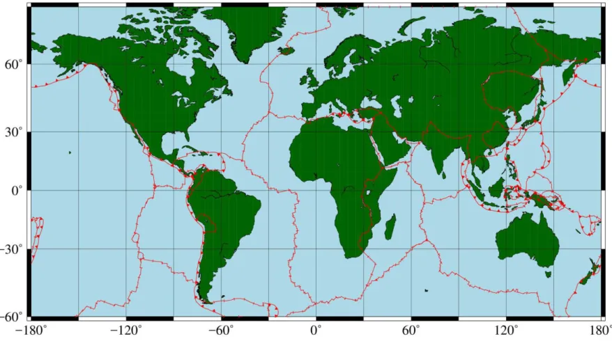
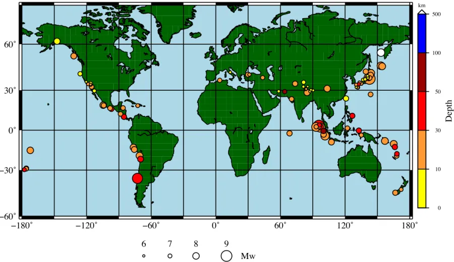
Figure 2.1 shows the geographical distribution of the earthquakes in our global

catalogue. Each event is represented by a circle with diameter growing with the magnitude and whose colour is an index of depth. As expected, earthquakes are mostly concentrated along the boundaries of the main tectonic plates in which the Earth’s lithosphere is fragmented (see Figure 2.2).

(15)

(16)

(17)

Table 2.1 shows the number of total events and the number of available FFMs from

1990 to 2015 per range of magnitude. Considering all the events with magnitude larger than 6, the percentage of FFMs we found is only 4.40%, which is quite small. It is to be noticed, however, that the percentage changes very much with the earthquake size. Indeed, for the events in the interval 6 ≤ MW < 7 the percentage is just 0.98%, while for

the ranges 7 ≤ MW < 8 and Mw ≥ 8, the percentage increases respectively to 30.65%

and to 87.5%. These figures highlight very well that the objects of the finite-fault inversion studies are mostly the large earthquakes: this can find a reason in the fact that large earthquakes are recorded by a larger number of stations and hence documented by a larger amount of instrumental data and observations.

Table 2.1: Frequency of FFMs and of earthquakes per magnitude classes

Finite-Fault Models Number of

Events

MW≥ 6 155 3521

6 ≤ MW < 7 31 3161

7 ≤ MW < 8 103 336

Mw ≥ 8 21 24

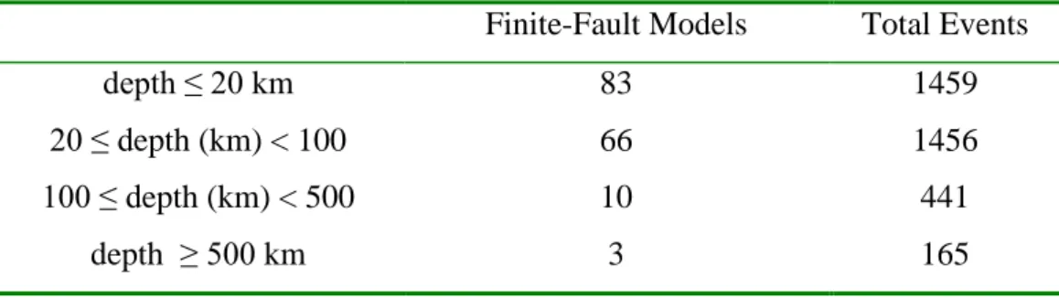
Table 2.2 shows the frequency of FFMs and earthquakes per hypocentre depth ranges.

For both categories, the frequency decreases with the increase of depth. The highest percentage of FFMs is 5.69% and refers to shallow events with depth ≤ 20 km.

Table 2.2: Frequency of FFMs and all earthquakes per hypocentre depth classes

Finite-Fault Models Total Events

depth ≤ 20 km 83 1459

20 ≤ depth (km) < 100 66 1456

100 ≤ depth (km) < 500 10 441

(18)

Table 2.3 gives the number of earthquakes that occurred in some selected regions, i.e.

the Andean domain, the Japanese region, the Mediterranean, and the Indonesian region. The choice of these areas derives from their high seismic potential, with the exception of the Mediterranean domain, which has been selected since it is our region where we aspire to apply some of the outcomes resulting from this work.

The majority of the FFMs collected referred to the Indonesian region (12.76%), and second, really close, one finds the Mediterranean (12.50%).

The boundaries of these areas have been drawn in a rough way, i.e. by means of simple rectangular polygonal lines specified by assigning latitude and longitude of the vertices.

Table 2.3: Frequency of earthquakes in selected areas

Finite-Fault Models Total Events

Andean domain 14 244

Japan 21 398

Mediterranean 5 40

Indonesia 25 196

In the next pages some graphs are given that show what has been partly summarized in the previous tables, and add some new statistics.

Figure 2.3, expanding the magnitude distribution given in Table 2.1, shows the number

of events per magnitude classes, from 1990 to 2015. Starting from MW = 6, magnitudes

are partitioned in bins of MW = 0.2. It is evident the decrease of the number of

earthquakes with the increasing of the magnitude, according to the Gutenberg-Richter law. The top-histogram in in Figure 2.3 simply shows the number of events with the increase of magnitude. The bottom graph, instead, presents the number of events on the vertical axe in logarithmic scale: the red dots plotted are the values of the above histogram, making them correspond to the central value of the membership magnitude step.

It is evident the correlation between Log(N) and MW (N is the number of the event for

that particular magnitude value). On the graph the values of the regression laws are also reported. The trend is in agreement with the Gutenberg-Richter law:

(19)

In our case, b = 1.15.

Figure 2.3: Number of events per magnitude classes

Figure 2.4 illustrates exactly what is reported in Table 2.2, providing a visual

representation of the FFMs distribution for the different classes of magnitude.

Figure 2.5 shows the time distribution of the FFMs earthquakes, year by year, with the

distinction in magnitude (6-7-8). It can be seen that there has been a growth of the available FFMs especially for earthquakes with Mw larger than 7. It can be also observed that in the last years (2014, 2015) the number slightly declines. In practice, it is expected that nowadays for each large earthquake at least one FFM is calculated, but

(20)

the final model is available in the databases with some delay that can even be as long as 1-2 years.

(21)

Figure 2.5: FFM events vs. time in the interval 1990-2015

Figure 2.6 and Figure 2.7 show what is summarized in Table 2.3 with the distinction

per magnitude classes. From Figure 2.7 one can notice that there are no events with FFM in the range 6 ≤ MW < 7 for the Indonesian region and in the range MW ≥ 8 for the

Mediterranean. The Andes region presents just one FFM event with magnitude lower than 7.

Comparing the two Figures, it is very interesting to observe that all the events with magnitude larger than 8 have a corresponding FFM (except one in Indonesia). The range 7 ≤ MW < 8, instead, is perfectly covered only for the Mediterranean and

Indonesian regions. The four areas are also delineated with rectangles on the map of

(22)

(23)

(24)

Figure 2.8: Geographical distribution of the FFM earthquakes

2.3 Finite Fault Model catalogues

Finite-fault inversions have become a topic of increasing interest in seismological research, since they allow a better understanding of the rupture mechanism and rupture evolution on the seismic fault. The data used in inversions can be of different types. They may be geodetic data of final deformation, in which case source inversions put constraints on the fault geometry and on the static slip distribution (i.e. the final displacements over the fault surface) (Mai and Thingbaijam, 2014).

Often, joint inversions, which combine available geodetic, seismic, tectonic (and when it is the case also tsunami) data, are also conducted, in order to match all the observations and provide a more detailed representation of the rupture process. Some joint inversions use all data simultaneously. Others, instead, follow an iterative approach where one set of observations is used to build an initial (prior) model for following inversions using other available data. The field of finite-fault inversion was pioneered in the early 1980s (see Olson and Apsel, 1982; Hartzell and Heaton, 1983). Subsequently, the method has been applied to numerous earthquakes (e.g., Hartzell,

(25)

1989; Hartzell et al., 1991; Wald et al., 1991; Hartzell and Langer, 1993;Wald et al., 1993; Wald and Somerville, 1995), while additional source-inversion strategies were developed and applied (e.g., Beroza and Spudich, 1988; Beroza, 1991; Hartzell and Lui, 1995; Hartzell et al., 1996; Zeng and Anderson, 1996).

Finite-fault source inversions highlight the complexity of the earthquake rupture process. The source images obtained give useful information, although with a restricted spatial resolution, of earthquake slip at depth, and potentially also on the temporal rupture evolution. Therefore, they result really important for additional work on the mechanics and kinematics of earthquake rupture processes. Hence, they play an important role in our comprehension of earthquake source dynamics.

It is beyond the scope of this thesis to treat and discuss source-inversion methods, that are the basis of the FFMs we use. In the next sub-sections we summarize the main data sources from which these models were taken.

2.3.1 USGS

The United States Geological Survey (USGS, formerly simply Geological Survey) is a scientific agency of the United States government. The organizational structure is divided into four main areas: concerning biology, geography, geology, and hydrology. The scientists of the USGS study the landscape of the United States, its natural resources, and the related natural hazards.

Many FFMs taken from USGS database and considered in the statistics are supplied by the National Earthquake Information Centre (NEIC) of United States Geological Survey. Further, several American universities are among the major contributors of these models.

2.3.2 UCSB database

This database includes a collection of rupture processes of large earthquakes (Mw>7) and interesting local events, inverted by means of the Ji's finite-fault inverse method. Only the results of recent earthquakes are provided. This work is supported, in turn, by the National Earthquake Information Center (NEIC) of the United States Geological Survey. The web page is built and maintained by Dr. C. Ji at UCSB (University of California, Santa Barbara).

(26)

(http://www.geol.ucsb.edu/faculty/ji/big_earthquakes/home.html)

2.3.3 Caltech

The California Institute of Technology (Caltech) has established the Tectonics Observatory in order to provide a new view of how and why the Earth's crust and lithosphere are deforming over time scales ranging from a few tens of seconds (the typical duration of an earthquake), to tens of millions of years (the time it takes to build mountains).

The Tectonics Observatory team has developed numerical models to estimate the location and amount of slip on an earthquake fault. They analyse all large earthquakes, as well as smaller ones that occur in areas of special interest to the Tectonics Observatory (http://www.tectonics.caltech

.edu /slip_history/).

2.3.4 SRCMOD

SRCMOD website is an online database of finite-fault rupture models of past earthquakes. These earthquake source models are obtained from inversion or modelling of seismic, geodetic and other geophysical data, and characterize the space-time distribution of kinematic rupture parameters. (from http://equake-rc.info/SRCMOD/). The current version of SRCMOD, directly accessible at http://equake-rc.info/SRCMOD/, provides to earthquake scientists, source modellers, and any interested user open access to more than 300 earthquake rupture models corresponding to about 100 earthquakes, in a unified representation, published over the last 30 years. The website is built on a three-tier architecture, which comprises client-side software (data presentation), server-side coding (data processing), and the back-end data storage. Three are the file formats the primary data for the source models are stored in: 1) MATLAB (http://it.mathworks.com/products/matlab) structures (.mat files), 2) ASCII files containing finite-source parameters (.fsp files), 3) ASCII files containing a comprehensive slip model (.slp files).

(27)

The entire database represents an inhomogeneous global collection of earthquake rupture models. Inhomogeneous in the sense of:

- faulting type

- location of the earthquake and, consequently

- tectonic province (interplate, intraplate, subduction) - data and observations used in the source inversion - inversion techniques applied

- available rupture-model information provided by the authors

- model parameterizations selected and modelling choices made by the modellers. A finite-fault (also known as kinematic) rupture model typically comprises several parameters, which include the final slip, rise time (duration of slip), rupture-onset time, and rake (angle of slip direction) (Mai and Thingbaijam, 2014). The source studies do not always invert for all these parameters. Some of them could have been fixed/assumed in advance, depending on data and the used inversion technique. The parameters may vary spatially: they are defined at node points or subfaults that constitute the rupture surface. In case of inversions using seismic data, the source time function describes the temporal slip evolution on each point of the fault and is typically chosen using a simple parametric shape or as a linear combination of many elementary slip functions (so-called multi time-window inversions) (Mai and Thingbaijam, 2014).

The spatial resolution of the model is defined by the size of the subfaults (or spacing of node points); typically, the details of the rupture process are resolved at a larger scale as a result of the chosen smoothing constraints or regularization (to handle the ill-posed inversion problem) and the trade-off between parameters (Mai et al., 2007; Monelli et al., 2009).

Thanks to the increased availability of seismic and geodetic networks, the FFM of recent earthquakes are higher detailed comparing to those of the previous decades. The number of available source models is also affected by the contribution of fast FFMs, generated from the so-called fast finite-fault inversions in a semi-automated way within hours of a sizeable earthquake and then published online on institutional web pages. But more accurate models are available with some delay, typically after several months. Scientific projects or institutions that deliver online rupture models (not only fast

(28)

(http://earthquake.usgs.gov/earthquakes/eqinthenews/; last accessed August 2016), source models of large earthquakes at Caltech (http://www.tectonics.caltech.edu/slip_history/index.html; last accessed August 2016), database of big earthquakes at University of California–Santa Barbara (http://www.geol.ucsb.edu/faculty/ji/big_earthquakes/ home.html; last accessed August 2016), and source process of recent earthquakes at University of Tsukuba (http://www.geol.tsukuba.ac.jp/ ~yagi-y/eng/earthquakes.html; last accessed August 2016).

The variability in rupture models is affected by the variety of source-inversion methods and available data. Furthermore, in the current database several earthquakes have more than two rupture models. There can be a significant variability between different source models for the same event. Multiple models are available, for example to name a few, for the 1992 Landers, the 1995 Kobe, the 1999 İzmit, the 2004 Sumatra, the 2008 Wenchuan and the 2011 Tohoku earthquakes. However, the nominal uncertainties of each of the source inversions are not well known. This has been pointed out previously (e.g., Beresnev, 2003) and can be understood in the context of the data used, the model parameterizations chosen, and the inversion techniques applied in such studies (Cohee and Beroza, 1994; Das and Suhadolc, 1996; Henry et al., 2000; Graves and Wald, 2001; Yokota et al., 2001; Delouis et al., 2002).

Regarding the characteristic reported for every event, the earthquake source dimensions (i.e., length, width or area) are generally estimated prior to the inversion from the spatial distribution of aftershocks. Regarding the rupture width, the thickness of the seismogenic crust is often used to constrain it. In other cases the fault plane size is estimated using source-scaling relationships.

However, the inversion procedures commonly assume conservatively large source dimensions, so that the entire rupture can be accommodated, which leads to an overestimation of the rupture sizes with small (even zero) displacements at the fault boundaries. Thus, it is necessary to trim the rupture model by eliminating superfluous small slips at the fault edges (Mai and Thingbaijam, 2014). In the following chapter we will discuss about this procedure.

(29)

As already pointed out in section 2.1 the main analyses carried out in this thesis work are based on FFM of the SRCMOD database. The main reasons are that SRCMOD is a collector of models also from other databases, that are incorporated after accurate quality check, and that it is a user-friendly online platform, easy to use.

(30)

3 Chapter 2

In this chapter a set of earthquake source-scaling relations between geometrical properties of the seismic fault and magnitude are obtained. Such relationships are often used from seismologists and engineers in seismic hazard and risk assessments. They are also used in the frame of tsunami hazard studies, and even in the common tsunami early warning practice, where typically from the earthquake location and magnitude (available in a few minutes after the quake) one makes real-time assessment on the generated tsunami. Indeed, the source parameters of an earthquake have a significant influence on tsunami generation, as pointed out in the Introductory chapter. The detailed features of the seismic source and the heterogeneous distribution of slip along the fault plane influence the initial tsunami field, which reflects on the tsunami propagation and on the tsunami effects on the coast.

We analyse the scaling laws relating the magnitude (MW) on one side, and some of the

main fault properties such as rupture length (Length), rupture width (Width), rupture area (Area), maximum displacement (MD) and average displacement (AD).

As already said in the previous chapter, all FFMs we analyse are taken from SRCMOD. The total number of FFMs we considered is 98.

Every model provides the geographical coordinates of the epicentre, the hypocentre depth, the rupture width and length, the seismic moment, the magnitude. The spatial variations of the on-fault slip along the strike and down-dip directions is also provided. The slip values are assigned over a matrix of sub-faults, with assigned number of rows (Nx) and columns (Nz). The dimensions (inDx, inDz) of the rectangle covering the entire fault are also given.

3.1 Fault size

The problem of the fault size evaluation is a sensitive issue. Establishing the rupture size of a fault (fault length or fault width) is not easy. If surface rupture occurred, for example, the fault length can be derived from the visible surface-rupture length. Alternatively, it can be estimated from the spatial extent of early aftershocks. However, these two approaches can give substantially different results (Wells and Coppersmith, 1994). As for the width, the determination of the fault width relies on aftershock only,

(31)

or, which is often the case of large strike-slip earthquakes, on the thickness of the seismogenic layer (Scholz, 1994).

Hence, the main errors in the evaluation of the fault dimension parameters can be found in the temporal evolution of the aftershock zone, in the accuracy of aftershock locations in 3D, in the interpretation of the initial extent of the aftershock sequence, in the reliability of the modelling.

As we already mentioned previously, in general, a variable slip distribution over an earthquake fault plane is obtained by inverting some kind of seismic, geodetic, tsunami, etc. data. In some cases, only one type of data is inverted, while in other cases joint inversions of different datasets are carried out. In all cases, typically, the overall dimension of the fault area to be discretized in the inversion procedure is pre-assigned based on some accepted criterion, such as general scaling laws relating earthquake magnitude and total fault area. It may happen that the predefined fault area is larger than needed.

Hence, depending on the inversion algorithm accuracy and on the quantity, quality and spatial distribution of the data to be inverted, the resulting slip matrix, that is the variable slip over the discretized rupture plane, may exhibit rows and/or columns full of zeroes along the edges. In those cases, the rupture length and width reported by the FFMs overestimate the true dimensions.

In order to get an image of the fault area affected by the seismic dislocation, we operated directly on the slip matrix with the following criterion: if there is an empty (i.e. full of zero slip values) row and/or column on the edges, we simply delete it.

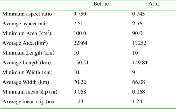
Somerville et al. (1999), instead, suggested to remove from all models any rows or columns for which the mean slip was lower than a determined fraction (0.3) of total average slip. This criterion seems to be too drastic, at least for the purpose of our work. The removal of part of the fault plane from the FFM implies a corresponding update of the fault dimensions. Table 3.1 contains the minimum and average values of aspect ratio, area, length, width, mean slip before and after the filtering procedure.

Initial rupture length and width are provided by the authors of the FFM. Area and aspect ratio were directly derived from those values. The mean slip was calculated as the mean over the slip matrix given by the authors in the “slp.txt” file.

(32)

The final average aspect ratio (where the average is meant over all the 98 faults examined) is larger than the original one: this is due to the fact that there is a higher alteration of the down-dip dimension (Wafter/Wbefore = 0.941) than of the along-strike one

(Lafter/Lbefore = 0.995).

Regarding the distribution of the slip, one can notice that after the trimming procedure there is an increase of 0.8 % in the average slip value.

Table 3.1: Earthquake source average geometric parameters before and after the filtering procedure

Before After

Minimum aspect ratio 0.750 0.745

Average aspect ratio 2.51 2.56

Minimum Area (km2₎ _100.0 _90.0 Average Area (km2) 22864 17252 Minimum Length (km) 10 10 Average Length (km) 150.51 149.81 Minimum Width (km) 10 9 Average Width (km) 70.22 66.08

Minimum mean slip (m) 0.068 0.068

Average mean slip (m) 1.23 1.24

3.2 Control of the models

The procedure of deleting the empty rows and columns on the edges does not exclude the possibility for some solutions to have many empty cells on the fault's plane or to present some very small values on the edges that do not permit to remove the edge itself. This implies some additional control. For each model the percentage of zero (Pz) slip values (Figure 3.2) in the matrix has been computed and, when higher than 50%, has been taken as an index of a possible anomaly, that required an individual visual checking.

This further control has led us to remove 5 anomalous FFM and to replace one FFM with another one available from a different author. The final number of FFM of our database is 98, that are the ones listed in Table 3.3.

(33)

Figure 3.2: Frequency of models per classes of Pz

Below one can find the list of the anomalous events that after the visual check were either removed or modified. Usually these events are characterised by some isolated cells with small slip values that are on the edge of the fault. Killing these cells has the effect that a full row or a full column turns out to be empty and can be removed. If this “blanking” procedure produces a fault model with an empty cell percentage that is still too high (larger than 50%), the fault is removed from the database, otherwise it is kept and labelled as modified in the list below.

3.2.1 Removed Events

1994-06-05 Taiwan (Ma and Wu, 2001) Mw=6.28

It shows an isolated cell with slip of 0.39 m in the bottom right corner. Killing it and the corresponding row, lowers Pz from 80% to 70%, which is not enough.

(34)

1995-09-14 Mexico (Corboulex, 1997) Mw=7.3

After replacing in the last column two 0.10 m slip values with 0.0, Pz passes 65% to 64%.

2006-12-26 Taiwan (Yen et al., 2008) Mw=6.8

Replacing a 0.05 m slip in the second last row with a 0.0, produces a resulting Pz = 77%, which is still too high.

2007-12-09 Indonesia (Konca et al., 2008) Mw=7.9

Replacing a 0.08 m slip in the first column with a 0.0, there has been a change from Pz= 62% to 61%.

2013-04-16 Kashmir, Iran (Wei, 2013) Mw=7.8

Without anything to delete Pz remains equal to 54%.

To help understand the process, in Figure 3.1 it is shown, as an example, the FFM by Ma and Wu (2001) of 05/06/1994 earthquake in Taiwan.

It is immediate to notice that most of the matrix cells are zero-slip (Pz=80%), and that Pz could not be reduced to less than 50% even after correcting the edge slip values.

(35)

Figure 3.1: Image of one of the removed events

3.3 Events with more than one solution

Some of the events considered have more than just one FFM, which poses a problem of selection. Generally, we have selected the most recent solution, but sometimes, cross-checking different fault representations, we have made a different choice. With events with a high number of solutions, such as the 11/03/2011 Tohoku, Japan, those models that presented solutions very different from the average have been rejected.

Often, one of the discriminating criteria was the degree of fullness of the FFM slip matrix. In particular, for the event of 15/08/2007 in Peru, we noticed the lack of slip values different from zero in a significant portion of the matrix (Figure 3.2, left image) only after we made the visual control. So the FFM was removed from our database and an alternative model was included. The two models are shown, one next to the other, in

(36)

Figure 3.2: FFMs of the 2007 Peru earthquake by two different authors. On the left, the discarded model; on the right, the chosen model

The next two figures show the frequency of FFM per classes of Pz in the final dataset of 98 FFMs, (Figure 3.3) and similar statistics for slip values lower than 1 cm (Figure

3.4): for this latter case we show statistics for all the events (top-left histogram), and

also for distinct magnitude classes: 6 ≤ Mw < 7 (top-right), for 7 ≤ Mw < 8 (bottom-left) and for Mw ≥ 8 (bottom-right).

As many as 42 FFMs exhibit Pz ≤ 5% of zero slip values in the slip matrix. Only 23 events have Pz larger than 25%, which means that for the remaining 75 FFMs, the zero-slip cells occupy less than a quarter of the fault plane.

(37)

Figure 3.3: Frequency of the zero-slip cells in the set of the selected models

Figure 3.4 (first histogram) shows that about one half of FFMs exhibit a percentage of

weak slip (lower than 1 cm) cells between 0-5%. It is interesting to note that there is not a great difference between the magnitude range 7 - 8 histogram (top-right) and the range 6 - 7 histogram (bottom-left). Instead, the histogram for the largest earthquakes (Mw ≥ 8) is somewhat different: here the highest percentage is smaller than 20%, and just 4 over 16 events present a percentage larger than 10%.

(38)

Figure 3.4: Histograms of the percentage of the small-slip ( < 1cm) cells for different classes of magnitude

(39)

The next two graphs (Figure 3.5, Figure 3.6) show the distribution of the selected 98 FFMs per magnitude and slip type. From Figure 2.7 it is evident that the majority of the earthquakes fall in the range 7 ≤ MW≤ 8 with a peak of 14 events centred in 7.5, while

13 events have magnitude larger than 8.

Figure 3.5: Number of FFMs per classes of magnitude (step = 0.2 Mw)

Figure 3.6 shows how many models fall in one the defined slip-type categories: 11

normal, 22 strike-slip, 32 reverse and 33 oblique events. The categories are defined here according to the slip rake. An earthquake with slip rake falling in a 10°-interval centred on 90° (-90°) is considered a reverse (normal) event. Further an earthquake with slip rake falling in a 10°-interval centred either on 0° or on 1800° is considered a strike-slip event. The “oblique” category includes all the events that do not belong to the other categories. Within the same mechanism, the events are divided into 3 classes of

(40)

magnitude (6 ≤ MW ≤ 7, 7 ≤ MW≤ 8, MW≥ 8): for every slip type the intermediate class

is the one with the highest number of events.

Figure 3.6: Number of FFMs per faulting style and magnitude

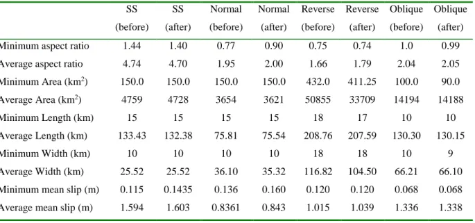
Below, in Table 3.2, it is repeated what was already reported in Table 3.1, but distinguishing between the different slip types. In this way, it is possible to highlight some facts. The strike-slip events are those with the lowest width (25.52 km), and consequently the largest average aspect ratio (4.74), while dip-slip events present the lowest values (in particular 1.79 for the reverse ones).

The dip-slip events (normal and reverse) are the most altered by the trimming procedure and the down-dip dimension is more altered than the along-strike one. Indeed, the new aspect ratio for dip-slip events is higher than the original one. For the strike-slip earthquakes the opposite happens: the final average aspect ratio is smaller than the original one.

(41)

Regarding the slip distribution, the strike-slip events are those with the higher mean slip (1.59 m), but the reverse ones are those with the largest variation, increasing the average value of 2.3%.

Table 3.2: earthquakes' source average geometric characteristic before and after the trimming procedure for different slip-type

SS (before) SS (after) Normal (before) Normal (after) Reverse (before) Reverse (after) Oblique (before) Oblique (after)

Minimum aspect ratio 1.44 1.40 0.77 0.90 0.75 0.74 1.0 0.99

Average aspect ratio 4.74 4.70 1.95 2.00 1.66 1.79 2.04 2.05

Minimum Area (km2₎ _150.0 _150.0 _150.0 _150.0 _432.0 _411.25 _100.0 _90.0 Average Area (km2₎ ₄₇₅₉ ₄₇₂₈ ₃₆₅₄ ₃₆₂₁ ₅₀₈₅₅ ₃₃₇₀₉ ₁₄₁₉₄ ₁₄₁₈₈ Minimum Length (km) 15 15 15 15 18 17 10 10 Average Length (km) 133.43 132.38 75.81 75.54 208.76 207.59 130.30 130.15 Minimum Width (km) 10 10 10 10 18 18 10 9 Average Width (km) 25.52 25.52 36.10 35.32 116.82 104.50 66.21 66.10 Minimum mean slip (m) 0.115 0.1435 0.136 0.160 0.120 0.120 0.068 0.068 Average mean slip (m) 1.594 1.603 0.8361 0.843 1.015 1.039 1.336 1.338

3.4 The models of the study

Table 3.1 summarizes some of the main features of the earthquakes and related FFMs.

An Identification Number (I.N.) is reported for each model as well as: occurrence date and slip type, magnitude, seismic moment, hypocentre depth, rupture dimensions and area, maximum and average displacement. In the last column of the Table the author/authors of the FFM are also given.

Below this table, Figure 3.7 represents all the models under study on the same global map: each of them is drawn with a circle whose diameter is proportional to the magnitude and whose colour is an index of depth.

(42)

Table 3.3: Finite-Fault Models used in this study

I. N. Location Date (m/d/y) Slip

Type Mw Mo Depth (km) L (km) W (km) Area (km2₎ MD _(m) AD _(m) References

1 Joshua Tree (Calif.) 04/23/1992 SS 6.2 2.70E+18 12.5 28 20 560 0.84 0.14 Bennet et al. (1995) 2 Landers (Calif.) 06/28/1992 SS 7.2 7.20E+19 7 76 15 1140 6.77 1.91 Zeng and Anderson (2000) 3 Tibet, Pumqu-Xainza 03/20/1993 O 6.3 2.97E+18 8.25 30 22 660 0.52 0.14 Wang et al. (2014)

4 Hokkaido-nansei-oki (Japan) 07/12/1993 R 7.6 2.85E+20 20 200 70 14000 4.36 0.62 Mendoza and Fukuyama (1996) 5 Northridge (Calif.) 01/17/1994 R 6.7 1.30E+19 17.5 17.5 23.5 412 4.14 0.76 Zeng and Anderson (2000) 6 Sanrikuki (Japan) 12/28/1994 R 7.7 3.99E+20 10 110 140 15400 4.03 0.71 Nagai et al. (2001) 7 Kobe (Japan) 01/16/1995 SS 6.8 1.76E+19 14 52 20 1040 2.75 0.50 Cho and Nakanishi (2000) 8 Colima (Mexico) 10/09/1995 R 8.0 9.67E+20 16.55 200 100 20000 4.77 1.18 Mendoza and Hartzell (1999) 9 Tibet, Pumqu-Xainza 07/03/1996 O 6.1 1.49E+18 8.25 25 18 450 0.45 0.10 Wang et al. (2014)

10 Hyuga-nada1 (Japan) 10/19/1996 R 6.8 1.84E+19 11.6 32.12 32.12 1032 2.92 0.54 Yagi et al. (1999) 11 Nazca Ridge (Peru) 11/12/1996 O 7.8 6.57E+20 21 180 120 21600 4.37 0.49 Salichon et al. (2003) 12 Hyuga-nada2 (Japan) 12/02/1996 R 6.7 1.19E+19 20.4 29.2 29.2 853 1.65 0.42 Yagi et al. (1999) 13 Kagoshimaen-hoku-seibu (Japan) 03/26/1997 SS 6.1 1.50E+18 7.6 15 10 150 0.87 0.34 Horikawa (2001) 14 Kagoshimaen-hoku-seibu (Japan) 05/13/1997 SS 6.0 1.16E+18 7.7 17 10 170 0.41 0.21 Horikawa (2001) 15 Antarctica (Strike-Slip Segment) 03/25/1998 SS 8.0 1.07E+21 12 290 35 10150 35.16 3.14 Antolik et al. (2000) 16 Antarctica 03/25/1998 O 7.8 4.85E+20 12 90 60 5400 21.10 2.83 Antolik et al. (2000) 17 Tibet, Pumqu-Xainza 08/25/1998 O 6.2 1.91E+18 8.25 38 23 874 0.20 0.07 Wang et al. (2014) 18 Iwate (Japan) 09/03/1998 O 6.3 3.20E+18 3 10 9 90 1.40 0.44 Nakahara et al. (2002) 19 Izmit (Turkey) 08/17/1999 SS 7.5 1.77E+20 16 160 28 4480 5.51 1.30 Cakir et al. (2004) 20 ChiChi (Taiwan) 09/20/1999 O 7.6 3.11E+20 7 78 39 3042 11.90 3.75 Sekiguchi et al. (2002) 21 Oaxaca (Mexico) 09/30/1999 N 7.5 1.82E+20 39.7 90 45 4050 2.46 0.64 Hernandez et al. (2001) 22 Hector Mine (Calif.) 10/16/1999 SS 7.1 5.82E+19 7.5 54 18 972 9.46 1.81 Salichon et al. (2004) 23 Duzce (Turkey) 11/12/1999 SS 6.7 1.28E+19 10 40.95 12.6 516 5.09 0.93 Birgoren et al. (2004) 24 Tottori (Japan) 10/06/2000 SS 6.7 1.40E+19 14.5 32 20 640 3.21 0.62 Semmane et al. (2005)a 25 Bhuj (India) 01/26/2001 R 7.4 1.33E+20 20 60 35 2100 12.44 1.51 Antolik and Dreger (2003) 26 Geiyo (Japan) 03/24/2001 R 6.7 1.19E+19 46.46 30 18 540 2.40 0.67 Kakehi (2004)

27 Denali (Alaska) 11/03/2002 SS 7.9 7.08E+20 6 292.5 18 5265 10.57 4.25 Asano et al. (2005) 28 Colima (Mexico) 01/22/2003 R 7.5 2.30E+20 20 70 85 5950 3.14 0.61 Yagi et al. (2004 29 Boumerdes (Algeria) 05/21/2003 R 7.3 8.40E+19 16 64 32 2048 3.52 1.24 Semmane et al. (2005)

(43)

30 Carlsberg Ridge 07/15/2003 SS 7.6 2.82E+20 11.32 320 36 11520 3.16 0.55 Wei (Caltech, Carlsberg 2003) 31 Miyagi-hokubu (Japan) 07/25/2003 SS 6.1 1.80E+18 6.5 18 10 180 1.03 0.31 Hikima and Koketsu (2004) 32 Tokachi-oki (Japan) 09/25/2003 R 8.2 2.36E+21 25 120 100 12000 7.06 3.11 Koketsu et al. (2004) 33 Bam, Iran 12/26/2003 O 6.5 7.30E+18 8 25 20 500 1.62 0.48 Poiata et al. (2012a) 34 Irian-Jaya, indonesia 02/07/2004 SS 7.2 7.08E+19 11.23 100 28 2800 3.37 1.03 Wei (Caltech, Irian-Jaya 2004) 35 Zhongba, Tibet 07/11/2004 N 6.2 2.24E+18 10 20 22.27 445 0.69 0.16 Elliott et al. (2010)

36 Parkfield (Calif.) 09/28/2004 O 6.1 1.36E+18 8.26 36.1 11.9 430 0.52 0.10 Custodio et al. (2005) 37 Niigata-Ken Chuetsu, Japan 10/23/2004 R 6.6 1.07E+19 10.6 28 18 504 3.08 0.67 Asano and Iwata (2009) 38 Sumatra 12/26/2004 R 9.1 6.50E+22 35 1480 224 331520 11.43 2.94 Ammon et al. (2005) 39 Fukuoka (Japan) 03/20/2005 SS 6.6 1.15E+19 14 26 18 468 2.67 0.68 Asano and Iwata (2006) 40 Sumatra 03/28/2005 O 8.7 1.17E+22 25.69 380 260 98800 12.50 2.56 Shao and Ji (UCSB, Sumatra 2005) 41 Zhongba, Tibet 04/07/2005 O 6.2 2.24E+18 5.98 28 18.72 524 1.29 0.19 Elliott et al. (2010)

42 Northern California 06/15/2005 SS 7.2 7.08E+19 9.003 102 35 3570 2.96 0.67 Shao and Ji (UCSB, Northern California 2005) 43 Honshu, Japan 08/16/2005 R 7.5 2.00E+20 34.49 96 56 5376 1.32 0.22 Shao and Ji (UCSB, Honshu 2005)

44 Kashmir, Pakistan 10/08/2005 O 7.6 2.82E+20 10.51 126 54 6804 6.37 1.75 Shao and Ji (UCSB,Kashmir 2005) 45 Kuril Islands 11/15/2006 R 8.3 3.16E+21 25.85 400 137.5 55000 8.93 1.69 Ji (UCSB, Kuril 2006)

46 Kuril Islands 01/13/2007 O 8.1 1.58E+21 18.15 200 35 7000 20.25 7.02 Ji (UCSB, Kuril 2007) 47 Noto Hanto, Japan 03/25/2007 O 6.7 1.57E+19 9.62 30 16 480 5.07 1.09 Asano and Iwata (2011) 48 Solomon islands 04/01/2007 R 8.1 1.58E+21 11.6 300 80 24000 3.73 1.47 Ji (UCSB, Solomon Islands 2007) 49 Pisco, peru 08/15/2007 O 8.0 1.12E+21 29.41 192 108 20736 8.21 1.63 Ji and Zeng (Peru 2007) 50 Niigata-ken Chuetsu-oki 08/17/2007 N 6.6 1.60E+19 8.9 33.25 29.75 990 2.58 0.32 Cirella et al. (2008) 51 Bengkulu, indonesia 09/12/2007 R 8.5 6.70E+21 21.23 400 250 100000 5.22 1.21 Gusman et al. (2010) 52 Tocopilla, Chile 11/14/2007 R 7.8 5.82E+20 36.95 375 200 75000 2.99 0.22 Ji (UCSB, Tocopilla 2007) 53 Gerze, Tibet 01/09/2008 O 6.4 4.47E+18 7.5 20 19.65 393 1.96 0.37 Elliott et al. (2010) 54 Gerze, Tibet 01/16/2008 N 5.9 7.94E+17 4 15 10 150 0.88 0.20 Elliott et al. (2010)

55 Simeulue, Indonesia 02/20/2008 R 7.4 1.41E+20 24.8 152 112 17024 1.08 0.15 Sladen (Caltech, Simeulue 2008) 56 Yutian, Tibet 03/20/2008 N 7.1 5.01E+19 4.104 54 19.05 1029 5.14 1.50 Elliott et al. (2010)

57 Wenchuan, China 05/12/2008 O 8.0 1.41E+21 16 320 60 19200 8.01 3.21 Yagi et al. (2012) 58 Iwate Miyagi Nairiku 06/13/2008 N 7.0 3.65E+19 6.5 42.66 17.38 741 6.36 1.82 Cultrera et al. (2013) 59 Zhongba, Tibet 08/25/2008 O 6.7 1.26E+19 7.626 30 30.4 912 1.54 0.25 Elliott et al. (2010)

60 Kermedac Islands, new Zealand 09/29/2008 R 7.0 3.55E+19 39.5 70 70 4900 0.98 0.14 Hayes (NEIC, New Zealand 2008) 61 Sulawesi, Indonesia 11/16/2008 R 7.3 1.00E+20 25.5 120 56 6720 2.33 0.45 Sladen (Caltech, Sulawesi 2008)

(44)

62 Papua 01/03/2009 O 7.6 2.82E+20 34.59 120 96 11520 4.96 0.59 Hayes (NEIC, Papua 2009) 63 L'Aquila, Italy 04/06/2009 N 6.3 3.13E+18 8.639 30 22 660 1.36 0.19 Gualandi et al. (2013)

64 Offshore Honduras 05/28/2009 O 7.3 1.00E+20 13.51 180 36 6480 3.09 0.58 Hayes and Ji (Offshore Honduras 2009) 65 Fiordland, New Zealand 07/15/2009 O 7.6 2.82E+20 24.14 160 96 15360 5.57 0.63 Hayes (NEIC, New Zealand 2009) 66 Java, Indonesia 07/17/2006 R 7.8 6.77E+20 15 250 140 35000 2.12 0.66 Yagi and Fukahata (2011)

67 Gulf of California 08/03/2009 SS 6.9 2.51E+19 9.163 108 20.8 2246 2.32 0.31 Hayes (NEIC, Gulf of California 2009) 68 Samoa 09/29/2009 N 8.0 1.12E+21 16.85 180 49.08 8834 14.92 3.33 Hayes (NEIC, Samoa 2009) 69 Padang, Indonesia 09/30/2009 O 7.6 2.82E+20 80 54 45 2430 5.60 1.78 Sladen (Caltech, Padang 2009) 70 Vanuatu 10/07/2009 O 7.6 2.82E+20 35 91 60 5460 2.93 0.87 Sladen (Caltech, Vanuatu 2009) 71 Haiti 01/12/2010 O 7.0 3.55E+19 11 45 22.5 1013 3.72 1.45 Sladen (Caltech, Haiti 2010) 72 Maule, Chile 02/27/2010 O 8.9 2.51E+22 37 600 187 112200 12.90 4.05 Shao et al. (UCSB, Maule 2010) 73 El Mayor-Cucapah, Mexico 04/04/2010 SS 7.4 1.20E+20 10 120 16 1920 9.25 1.89 Mendoza and Hartzell (2013) 74 Northern Sumatra 04/06/2010 R 7.8 5.62E+20 30.64 240 216 51840 3.17 0.22 Hayes (USGS, Northern Sumatra 2010) 75 Northern Sumatra 05/09/2010 R 7.2 7.08E+19 44.63 90 90 8100 1.13 0.18 Hayes (NEIC, Northern Sumatra 2010) 76 Darfield, South Island New Zealand 09/03/2010 O 7.0 3.80E+19 10.83 80 26 2080 3.51 0.60 Hayes (NEIC, Darfield 2010) 77 Sumatra 10/25/2010 R 7.7 3.98E+20 17.43 375 196 73500 1.20 0.12 Hayes (NEIC, Southern Sumatra 2010) 78 Bonin Islands 12/21/2010 O 7.4 1.41E+20 17.77 110 42 4620 3.71 0.53 Hayes (NEIC, Bonin Islands 2010) 79 Vanuatu 12/25/2010 N 7.3 1.00E+20 15.17 90 42 3780 2.82 0.44 Hayes (NEIC, Vanuatu 2010) 80 Pakistan 01/18/2011 N 7.2 7.08E+19 66.79 60 60 3600 3.49 0.33 Hayes (NEIC, Pakistan 2011)a 81 Offshore Honshu, Japan 03/09/2011 R 7.3 1.00E+20 20.72 126 126 15876 1.35 0.19 Hayes (NEIC, Offshore Honshu 2011) 82 Tohoku-Oki, japan 03/11/2011 R 9.1 5.50E+22 21 525 260 136500 48.00 9.55 Wei et al. (2012)

83 Kermadec Islands 07/06/2011 N 7.3 1.00E+20 19.04 216 72 15552 4.62 0.34 Hayes (USGS, Kermadec Islands 2011) 84 Vanuatu 08/20/2011 R 7.3 1.00E+20 31.42 102 90 9180 0.93 0.12 Hayes (NEIC, Vanuatu 2011) 85 Kermadec Islands 10/21/2011 O 7.4 1.41E+20 32.1 90 90 8100 3.19 0.28 Hayes (NEIC, Kermadec Islands 2011) 86 Van,Turkey 10/23/2011 R 7.1 5.01E+19 19 95 40 3800 4.65 0.50 Konca (2015)

87 Sumatra 01/10/2012 SS 7.2 7.08E+19 18.37 90 21 1890 6.71 1.29 Hayes (NEIC, Sumatra 2012) 88 Oaxaca, Mexico 03/20/2012 R 7.4 1.41E+20 19.74 126 108 13608 4.53 0.28 Hayes (NEIC, Oaxaca 2012) 89 Sumatra 04/11/2012 SS 8.6 8.90E+21 22 384 60 23040 34.00 8.72 Wei (Caltech, Sumatra 2012)

90 Offshore El Salvador 08/27/2012 O 7.3 1.00E+20 19.85 210 128 26880 1.06 0.09 Hayes (NEIC, Offshore El Salvador 2012) 91 East of Sulangan, Philippines 08/31/2012 O 7.6 2.72E+20 34.04 128 90 11520 3.14 0.42 Hayes (USGS, Philippines 2012) 92 Costa Rica 09/05/2012 R 7.6 2.54E+20 39.32 150 120 18000 3.05 0.29 Hayes (NEIC, Costa Rica 2012) 93 Masset,Canada 10/28/2012 R 7.8 7.00E+20 17 210 90 18900 3.16 0.60 Wei (Caltech, Masset 2012)

(45)

94 Santa Cruz islands 06/02/2013 O 8.1 1.54E+21 12.7 144 90 12960 12.70 2.86 Lay et al. (2013) 95 Okhotsk Sea 05/24/2013 SS 8.3 5.02E+21 608 195 60 11700 9.92 3.82 Ye at al. (2013)

96 Scotia Sea 11/17/2013 SS 7.7 8.94E+20 10.72 392 50 19600 4.40 0.83 Hayes (USGS, Scotia Sea 2013) 97 Iquique, Chile 04/01/2014 O 8.1 1.58E+21 21.54 285 160 45600 4.21 0.67 Wei (Caltech, Iquique 2014) 98 Gorkha, Nepal 04/25/2015 O 7.9 9.09E+20 15 160 88 14080 7.53 2.48 Yagi and Okuwaki (2015)

(46)

(47)

3.5 Source scaling relationships

In Table 3.4 the regression formulas computed in this study for maximum slip (MD), mean slip (AD), fault length (Length), fault width (Width) and fault area (Area) versus moment magnitude (MW) are listed, divided into 5 categories: strike-slip events, reverse

events, normal events, oblique events, all events (2nd column).

The number of data points used in each case is shown in the 3rd column. The best estimates for the coefficients a and b are listed in the 4th and 5th columns, followed by the coefficients of correlation r and the standard error σ.

For the calculations and the regressions, the magnitude values were taken with two decimal figures. However, when considered individually as estimates of the moment magnitude, they are considered significant only to one decimal figure.

Table 3.4: Direct and inverse regressions between rupture dimensions (Length, Width), rupture area (Area), maximum displacement (MD), average displacement (AD), and moment magnitude (MW) (r is the correlation coefficient and σ is the standard error).

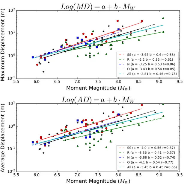
Equation Slip Type Number of events a b r σ MW = a+b *Log(MD) SS R N All Oblique 22 32 11 98 33 6.34 7.03 6.3 6.65 6.61 1.29 1.05 1.39 1.23 1.33 0.88 0.62 0.86 0.75 0.85 0.16 0.24 0.27 0.11 0.15 Log(MD) = a+b * MW SS R N All Oblique 22 32 11 98 33 -3.65 -2.20 -3.25 -2.81 -3.43 0.6 0.36 0.53 0.46 0.54 0.88 0.61 0.86 0.75 0.85 0.073 0.084 0.105 0.041 0.061

(48)

Equation Slip Type Number of events a b r σ MW = a+b *Log(AD) SS R N All Oblique 22 32 11 98 33 7.17 7.77 7.26 7.49 7.48 1.36 0.78 1.06 0.99 1.11 0.87 0.57 0.74 0.66 0.77 0.17 0.21 0.32 0.11 0.16 Log(AD) = a+b * MW SS R N All Oblique 22 32 11 98 33 -4.00 -3.36 -3.88 -3.45 -4.10 0.56 0.41 0.52 0.45 0.54 0.87 0.57 0.74 0.66 0.77 0.068 0.108 0.157 0.051 0.08 MW =a+b*Log(L) SS R N All Oblique 22 32 11 98 33 4.38 4.8 4.23 4.38 4.15 1.44 1.32 1.56 1.5 1.64 0.93 0.90 0.92 0.91 0.91 0.12 0.12 0.23 0.07 0.12 Log(L) =a+b* MW SS R N All Oblique 22 32 11 98 33 -2.39 -2.55 -2.00 -2.11 -1.73 0.60 0.62 0.54 0.56 0.50 0.93 0.90 0.92 0.91 0.91 0.052 0.054 0.079 0.026 0.042 MW =a+b* Log(W) SS R N All Oblique 22 32 11 98 33 3.75 4.67 4.33 4.84 4.31 2.51 1.52 1.77 1.49 1.80 0.83 0.81 0.74 0.8 0.87 0.38 0.21 0.53 0.11 0.18

(49)

Equation Slip Type Number of events a b r σ Log(W) =a+b * MW SS R N All Oblique 22 32 11 98 33 -0.61 -1.33 -0.69 -1.47 -1.40 0.27 0.43 0.31 0.43 0.42 0.83 0.81 0.74 0.8 0.87 0.041 0.058 0.094 0.032 0.043 MW = a+b *Log(A) SS R N All Oblique 22 32 11 98 33 3.86 4.54 4.01 4.29 4.03 1.0 0.75 0.91 0.84 0.91 0.94 0.89 0.88 0.91 0.92 0.08 0.07 0.16 0.04 0.07 Log(A) = a+b* MW SS R N All Oblique 22 32 11 98 33 -3.01 -3.88 -2.68 -3.58 -3.14 0.88 1.04 0.85 0.98 0.92 0.94 0.89 0.88 0.91 0.92 0.07 0.1 0.153 0.046 0.072

Let us first consider the relationships between the fault's dimensions and the magnitude. Regarding the length of the fault plane, it results highly correlated to the magnitude, with the stronger value of the correlation coefficient for the strike-slip events.

The width presents instead a lower slope. Contrary to the length case, strike-slip events have the lowest slope with respect to the other categories: this suggests an easier rupture propagation along the strike direction for strike-slip events.

The area of the fault also increases with the magnitude, with higher values and slopes for reverse earthquakes.

(50)

(51)

Figure 3.9: Regression laws of area and aspect ratio vs. magnitude

Considering the Maximum Displacement MD (Figure 3.10, top graph) one observes that it increases with the magnitude, but the correlation coefficient is not that high. The strike-slip events, for which the correlation coefficient has the highest value, generally exhibit a larger peak of slip, for a fixed magnitude, with respect to the other mechanisms.

Reverse earthquakes, instead, present the lowest value of slip peak.

The same considerations hold when one considers the average displacement (Figure

(52)

Figure 3.10: Regression laws of max and mean slip vs. magnitude

It results interesting to see if the slip correlates also with the fault dimensions. For this reason, the regression between mean slip and max slip with length is illustrated in

Figure 3.11. The graphs show that for the displacement vs length relationships the

correlation is weak (0.35 ≤ r ≤ 0.77 for MD, 0.2 ≤ r ≤ 0.69 for AD), and is higher for the strike-slip events (with the exception of MD vs. Length that has the highest correlation for the normal events). Hence, both slip and length correlate better with the magnitude.

(53)

Figure 3.11: Regression law of max and mean slip vs. rupture length

Taking into account that the most widely used scaling relations are those of Wells and Coppersmith (1994), it is interesting to make some comparisons with their results.

(54)

Table 3.5: Regression laws by Wells and Coppersmith (1994) Equation Slip Type Number of events a b r Standard Deviation MW =a+b*Log(L) SS R N All 93 50 24 167 4.33 4.49 4.34 4.38 1.49 1.49 1.54 1.49 0.96 0.93 0.88 0.94 0.24 0.26 0.31 0.26 Log(L) =a+b* MW SS R N All 93 50 24 167 -2.57 -2.42 -1.88 -2.44 0.62 0.58 0.50 0.59 0.96 0.93 0.88 0.94 0.15 0.16 0.17 0.16 MW =a+b* Log(W) SS R N All 87 43 23 153 3.80 4.37 4.04 4.06 2.59 1.95 2.11 2.25 0.84 0.90 0.86 0.84 0.45 0.32 0.31 0.41 Log(W) =a+b * MW SS R N All 87 43 23 153 -0.76 -1.61 -1.14 -1.01 0.27 0.41 0.35 0.32 0.84 0.90 0.86 0.84 0.14 0.15 0.12 0.15 MW = a+b *Log(A) SS R N All 83 43 22 148 3.98 4.33 3.93 4.07 1.02 0.90 1.02 0.98 0.96 0.94 0.92 0.95 0.23 0.25 0.25 0.24 Log(A) = a+b* MW SS R N All 83 43 22 148 -3.42 -3.99 -2.87 -3.49 0.90 0.98 0.82 0.91 0.96 0.94 0.92 0.95 0.22 0.26 0.22 0.24

Regarding the rupture length, our results are in agreement with those obtained by Wells and Coppersmith (1994).

(55)

For what concerns the rupture width and magnitude, because of differences in slope and/or intercept, our relations lead to higher width and area for the same magnitude. We have to take into account that Wells and Coppersmith (1994) considered a larger number of events, with magnitude also smaller than 6 and 5. This could explain why the length presents a more regular behaviour with the increase of the magnitude, while the width shows a different trend depending on the magnitude window taken into account.

Table 3.6 tests, in the case of rupture length, how close our results are to those by Wells

and Coppersmith (1994). The value of Length for the different slip types calculated for an MW = 7.5 is listed, as well the value of magnitude calculated for L = 150 km.

Table 3.6: Comparison on the length and magnitude values respectively predicted for a given magnitude or length

Calculated value Slip Type Wells and Coppersmith This study

L (km, MW = 7.5) SS R N All 120 85 74 97 129 126 112 123 MW (L = 150 km) SS R N All 7.57 7.73 7.69 7.62 7.51 7.65 7.62 7.64

From Table 3.6 it is evident that our regression laws give larger rupture length for every slip type. Again, it is important to highlight that our set of events regards only earthquakes with MW ≥ 6.

Figure 3.12 shows the relationship between seismic moment and magnitude. The two

are perfectly correlated, which suggests that in building the FFM the two quantities have been analytically derived one from the other according to the Hanks and Kanamori law. If one wants to compare the source dimensions with the seismic moment, we can proceed following the reasoning explained below.