A Two-Step Iterative Inexact-Newton Method for Electromagnetic Imaging of Dielectric Structures from Real Data

UNIVERSITY

OF TRENTO

DIPARTIMENTO DI INGEGNERIA E SCIENZA DELL’INFORMAZIONE

38123 Povo – Trento (Italy), Via Sommarive 14 http://www.disi.unitn.it

A TWO-STEP ITERATIVE INEXACT-NEWTON METHOD FOR ELECTROMAGNETIC IMAGING OF DIELECTRIC STRUCTURES FROM REAL DATA

C. Estatico, G. Bozza, A. Massa, M. Pastorino, and A. Randazzo

December 2005

A Two-Step Iterative Inexact-Newton Method

for Electromagnetic Imaging of Dielectric Structures from Real Data

C. Estatico,(1) G. Bozza,(2) A. Massa,(3) M. Pastorino,(2) and A. Randazzo(2) (1)

Department of Mathematics, University of Genoa, Via Dodecaneso 35, 16146 Genova, Italy.

e-mail: estatico@dima.unige.it (2)

Department of Biophysical and Electronic Engineering, University of Genoa, Via Opera Pia 11A, 16145 Genova, Italy,

Phone: +390103532242, Fax: +390103532245, e-mail: pastorino@dibe.unige.it, randazzo@dibe.unige.it (3)

Department of Information and Communication Technology, University of Trento, Via Sommarive 14, I-38050 Trento, Italy.

Phone: +39 0461882057 Fax: +39 0461881696 e-mail: andrea.massa@ing.unitn.it

Abstract −−−− A new inverse scattering method is assessed against some of the real input data measured by the Institut Fresnel, Marseille, France. The method is based on the application of an Inexact-Newton method to the Lippmann-Schwinger integral equation of the inverse scattering problem within the second-order Born approximation. The regularization properties of the approach are evaluated by considering the reconstruction of multiple dielectric cylinders.

1. Introduction

In the last years, the inverse scattering problem has been addressed by using several different approaches in order to face the various well-known problematic aspects (e.g., nonlinearity, ill-posedness, ill-conditioning, etc.).

Several inversion methods are now available [1]-[11], especially for two-dimensional configurations. They can be grouped into two main categories. The first one includes deterministic and stochastic methods aimed at facing the nonlinear equations of the inverse scattering problem without approximations different from the numerical ones. The second category includes simplified methods based on some kind of approximation.

The aim of the present paper is to assess (by using the new real data collected by the Institut Fresnel, Marseille, France) the reconstruction capabilities of a new inverse method, which combines

a regularization Inexact-Newton method with the inverse-scattering formulation developed in the framework of the second-order Born approximation.

Although accurate reconstructions could be expected only for weakly scattering objects, the new approach has been proven (through numerical simulations [12]) to be very efficient in regularizing the ill-posed inverse problem, particularly robust against the noise on the input data, and computationally efficient, since the internal distribution of the total electric field (or related quantities), which changes for each illumination, is not to be retrieved.

The results shown in the present paper represent the first validation of the approach against real experimental data.

The paper is organized as follows. In section 2, the inversion method is briefly outlined, whereas the results of the dielectric reconstructions of some sets of real input data are reported in Section 3. Finally, Section 4 draws some conclusions.

2. Mathematical Formulation

The dielectric properties of the investigation area (which includes the cross sections of the scatterers and is denoted by Ωinv) are represented by means of the complex contrast function χ(r), r ∈ Ωinv, which is defined as 1 ) ( ) (r =ε_r r − χ , (1)

where εr(r) is the complex relative dielectric permittivity at point r ∈ Ωinv.

Omitting the ejωt time dependence, the 2D-TM inverse scattering problem can be expressed by the following integral formulation

( )

r 2

( ) ( ) ( )

r () r r r r ( )

[ ]

( )

( )

r ) ( d , v _totv v tot v scatt k u g F u u inv χ χ ′ ′ ′ ′= − =

_∫

Ω , v = 1,…,V (2)

where u_tot(v)

( )

r denotes the unknown total electric field, superscript v indicates that the relative quantities are related to the v-th view, being V the total number of views, k is the free-space wavenumber given by k =ω ε₀µ₀ , and g

( )

r,r′ is the free-space Green’s function [13].

The electromagnetic inverse scattering problem consists in retrieving (a good approximation of) the complex contrast function χ, starting from the knowledge of the total electric fields u_meas(v)

( )

r , for v = 1,…,V, in a region of observation Ωobs located outside the investigation domain Ωinv. This inverse problem leads to the following nonlinear equation with respect to the unknown χ

( )

u

( )

u

( )

v V u

F[χ _tot(v)]r + _inc(v) r = _meas(v) r ,r∈Ω_obs, =1,.., , (3) where u_inc(v)

( )

r , r ∈ Ωobs, is the known incident electric field in the observation region related to the v-th illumination.

In this paper, the second-order Born approximation is exploited, i. e.,

( )

r 2 χ

( )

r ()

( )

r 2 χ

( ) ( ) (

r ( ) r r r

)

r

( )

r r r ( )

[ ]

χ

( )

r ) ( ~ d , d , v v inc v inc v scatt k u k u g g F u inv inv = ′ ′         ′ ′′ ′ ′′ ′′ − ′ ′ − ≅

_∫

_∫

Ω Ω . (4)

The solution of equation (3) is then recasted as the solution of the following equation

[ ]

( )

u

( )

u

( )

v V

F~(v) χ r + _inc(v) r = _meas(v) r ,r∈Ω_obs, =1,.., . (5) It is worth noting that, although equation (5) is still nonlinear, now the nonlinearity is limited to the contrast function. Furthermore, u_tot(v)(r), r ∈ Ωinv, is not needed, leading to a significant reduction in the computational load. In our approach, equation (5) is solved by using an iterative regularization method based on an Inexact-Newton scheme: At any step, equation (5) is first linearized (outer iteration), and the generalized solution of such a linear equation is approximated and regularized by using the iterative Landweber method [14] [15] for linear operators (inner iteration).

From (4), we can write that

(

)

_{( )}

( )

_{( )}

( )

2 ) ( ~ ~ _' ~ h h F F h F v + − v = v +Ο χ χ χ , (6)

where F~_χ(v)' is the Fréchet derivative of the operator F~(v) at the point χ, defined as follows

[

]

( )

[ ]

( )

_∫

( )

[ ]

( ) ( )

_∫

( )

[

]

( ) ( )

Ω Ω ′ ′ ′ ′ − ′ ′ ′ ′ − = inv inv g F h k g h F k h F h F~_χ(v)' r ₁(v) r 2 χ r ₁(v) r r,r dr 2 r ₁(v)χ r r,r dr , (7)

and F₁(v) denotes the first order Born approximation

[

]

( )

_∫

( ) ( ) ( )

Ω ′ ′ ′ ′ − = inv g u k F₁(v)χ r 2 χ r _inc(v) r r,r dr . (8)

Linearization (6) leads to the Newton method as follows. Let χ₀ be a complex contrast used as initial guess. For j = 0,1,... , compute χ_j+1 =χ_j +h_j, where h_j∈X solves the linear problem

( )

v V F u u h F v _{j meas}v _incv v _j j , 1,.., ~ ' ~( ) ₌ ( ) ₋ ( ) ₋ ( ) χ ₌ χ , (9)

and repeat until some pre-specified stopping rule holds true.

Since (4) involves Fredholm integral operators of the first kind onto the infinite dimensional space of all the contrast functions χ, equation (5) gives rise to an ill-posed inverse problem. It follows that any Newton step (equation (9)) can be posed, too, since it is a linear approximation of the ill-posed equation (5) under linearization (6) [16].

Under these arguments, instead of solving (9) directly, we search for a regularized solution of the normal, or least square, equation

( )

(

)

∑

∑

= = − − = V v v _j inc v meas v V j v v F u u F h F F j j j 1 ) ( ) ( ) ( * ) ( 1 ) ( * ) ( ~ ' ~ ' ~ ' ~ ν χ ν χ χ χ , (10) where as usual ~(v)'* j

F_χ denotes the adjoint operator of the Fréchet derivative ~(v)'

j

F_χ . As already mentioned, in the present paper we use the Landweber iterative regularization method. In this method, the number of iterations plays the role of a regularization parameter. Indeed, in the case of noisy data, it can be easily proven that the first iterations provide noise filtering, while the subsequent ones restore from components with higher noise, and then the iterative solution becomes more and more inaccurate [14]. Besides its easy implementation, it is known that this method presents very good regularization and robustness features (some recent applications can be found in [2][17]-[19]).

In order to apply the Landweber method to equation (10), let h_j,0 ≡0 be the initial guess and let

max

k be a pre-assigned total number of iterations. Compute, for a fixed convergence parameter

1 1 ) ( * ) ( ' ~ ' ~ 2 0 − =

∑

< < s V v v j F j F j ν χ χ τ (being s

L the spectral norm of L ), the iterative step

( )

(

)

[

]

∑

= + = − − − − V j v v inc v meas k j v v j k j k j h F F h u u F h j j 1 ) ( ) ( ) ( , ) ( * ) ( , 1 , ~ ' ~ ' ~ ν χ χ χ τ , (11)

then update k:=k+1 and repeat until k=kmax. In this way, the last Landweber iteration hj,k_max is a

regularized solution of the Gauss normal equation (10), that is,

max ,k j

h is a regularized approximation of the exact solution h of (10). It should be noticed that the proposed (two-steps) Newton-_j Landweber method is a (much faster) generalization of the classical (single-step) Landweber iterative method for nonlinear operators [15][16]. In particular, if k_max = 1, the proposed iterative scheme (9)-(11) and the Landweber iterative method for nonlinear operators are equivalent.

4. Numerical Results

In this section, some of the real input data measured by the Institut Fresnel, Marseille, France, are used to assess the proposed method. In particular, we consider the following configurations (TM wave scattering):

(a) A “foam” circular cylinder with contrast function value of χ1_obj =0.45. Inside the “foam” there is another circular dielectric cylinder of χ_obj2 =2 (FoamDielIntTM);

(b) Same as in (a), with the dielectric cylinder of contrast function χ_obj2 =2 located outside the “foam”;

(c) A combination of (a) and (b) (FoamTwinDielTM).

The investigation domain, Ωinv, is a square area of side l = 0.2 m, which is discretized by using a

grid of 40 × 40 square subdomains.

Since the approximation used in this work is mainly valid for weak scatterers, only the data collected at f ≤ 4 GHz are used in the reconstruction process. The accuracy of the reconstruction is evaluated by means of two following error parameters

inv inv obj obj Ω Ω − = χ χ χ γ (14) and

∑

= − Ω = V v v tot v tot obs u u 1 2 ) ( ) ( ~ κ , (15)

where χ and χ_obj are respectively the reconstructed and true contrast functions, (v) tot

u is the total measured electric field related to the v-th view, and u~_tot(v) is the correspondent electric field computed on the basis of the reconstructed contrast function χ. Here

inv Ω • and obs Ω • denote the classical discrete 2-norm in the investigation area and observation area, respectively. The first error parameter γ is the relative error on the dielectric reconstruction, while the second error parameter

κ is the discrepancy between actual and computed electric fields.

4.1 Configuration (a) (FoamDielInt)

As previously stated, the object under test is composed by a circular cylinder (with contrast function 45

. 0

1 =

obj

χ ) with embedded a second homogeneous circular cylinder with contrast function 2

2 =

obj

χ . The two cross sections have diameters 1 =0.08m

obj

d and 2 =0.03m

obj

d , and are centered

at r_obj1 =(0.0,0.0)m and r_obj2 =(−0.005,0.0)m, respectively.

The best values of the parameters kmax and jmax have been empirically determined by means of

jmax = 20 result in quite good solutions. It is worth noting that, in all cases, the initial guess χ0 of

contrast-function distribution for the outer iteration (9) corresponds to a completely empty investigation domain.

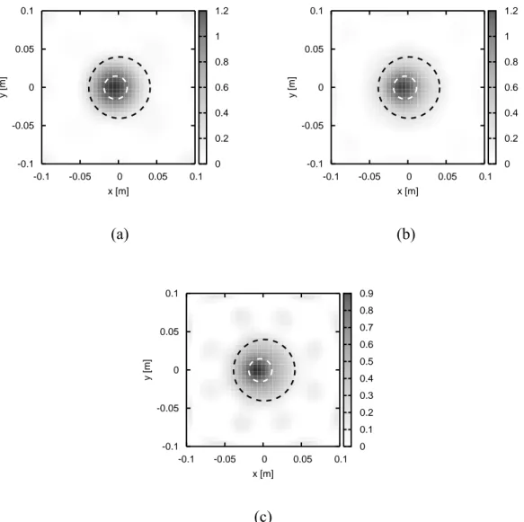
The results obtained by using these data are reported in Figure 1. As can be seen from this figure, the proposed method is able to obtain quite good results for the considered frequencies, especially for f = 2 GHz and f = 3 GHz. 0 0.2 0.4 0.6 0.8 1 1.2 -0.1 -0.05 0 0.05 0.1 x [m] -0.1 -0.05 0 0.05 0.1 y [m] 0 0.2 0.4 0.6 0.8 1 1.2 -0.1 -0.05 0 0.05 0.1 x [m] -0.1 -0.05 0 0.05 0.1 y [m] (a) (b) 0 0.1 0.2 0.3 0.4 0.5 0.6 0.7 0.8 0.9 -0.1 -0.05 0 0.05 0.1 x [m] -0.1 -0.05 0 0.05 0.1 y [m] (c)

Figure 1 – Reconstructed distributions of the contrast function χ for different values of the frequency. (a) f = 2 GHz; (b) f = 3 GHz; (c) f = 4 GHz.

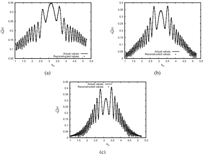
The samples of the electric field, both measured and computed on the basis of the reconstructed distribution of the contrast function, are reported in Figure 2 for the first view. In these graphs, the calculated values are very close to the measured ones in all cases. We remark that such a fitting of the input data is very important when dealing with iterative inverse scattering methods.

0.05 0.1 0.15 0.2 0.25 0.3 0.35 1 1.5 2 2.5 3 3.5 4 4.5 5 5.5 u (1) tot ( r ) θm Actual values Reconstructed values 0 0.05 0.1 0.15 0.2 0.25 0.3 0.35 0.4 1 1.5 2 2.5 3 3.5 4 4.5 5 5.5 u (1) tot ( r ) θm Actual values Reconstructed values (a) (b) 0 0.05 0.1 0.15 0.2 0.25 0.3 0.35 0.4 0.45 1 1.5 2 2.5 3 3.5 4 4.5 5 5.5 u (1) tot ( r ) θm Actual values Reconstructed values (c)

Figure 2 – Original and reconstructed electric fields (amplitude) at the measurement points for the first view. (a) f = 2 GHz; (b) f = 3 GHz; (c) f = 4 GHz.

Finally, the behaviors of the errors parameters γ and κ versus the outer iteration number are reported in Figure 3. 0.55 0.6 0.65 0.7 0.75 0.8 0.85 0.9 0.95 1 1.05 1.1 0 5 10 15 20 γ Iteration number, j q = 1 q = 2 q = 3 0 0.5 1 1.5 2 2.5 3 3.5 0 5 10 15 20 κ Iteration number, j q = 1 q = 2 q = 3 (a) (b)

Figure 3 – Behavior of the error parameters (a) γ and (b) κ versus the outer iteration number and for different values of the frequency, fq = (q + 1)109 Hz.

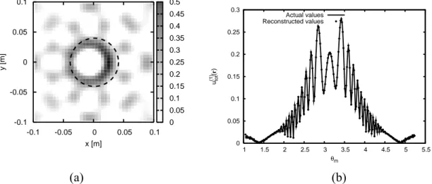
We point out that, for this first configuration, the data collected at frequency f = 5 GHz have been considered, too. The reconstructed distribution of the contrast function and the corresponding values of the electric field at the measurement points are reported in Figure 4. As expected, although there is a good agreement with the electric field data and the shape of the object is accurately determined, the overall reconstruction is rather poor.

0 0.05 0.1 0.15 0.2 0.25 0.3 0.35 0.4 0.45 0.5 -0.1 -0.05 0 0.05 0.1 x [m] -0.1 -0.05 0 0.05 0.1 y [m] 0 0.05 0.1 0.15 0.2 0.25 0.3 1 1.5 2 2.5 3 3.5 4 4.5 5 5.5 u (1) tot ( r ) θm Actual values Reconstructed values (a) (b)

Figure 4 – (a) Reconstructed distribution of the constrast function and (b) corresponding values of the electric field at the measurement points for the first view. f = 5 GHz.

4.2 Configuration (b) (FoamDielExt)

In this configuration, two circular cylinders are centered at r_obj1 =(0.0,0.0)m and m ) 0 . 0 , 055 . 0 ( 2 = − obj

r , respectively. The contrast functions of the two objects are 1 =0.45

obj

χ and

2

2 =

obj

χ , and the two cross sections have diameters d_obj1 =0.08m and d_obj2 =0.03m, respectively. In these reconstructions, too, the initial guess for the contrast function distribution is a void investigation domain.

0 0.1 0.2 0.3 0.4 0.5 0.6 0.7 0.8 0.9 -0.1 -0.05 0 0.05 0.1 x [m] -0.1 -0.05 0 0.05 0.1 y [m] 0 0.1 0.2 0.3 0.4 0.5 0.6 0.7 0.8 0.9 1 -0.1 -0.05 0 0.05 0.1 x [m] -0.1 -0.05 0 0.05 0.1 y [m] (a) (b) 0 0.1 0.2 0.3 0.4 0.5 0.6 0.7 0.8 0.9 -0.1 -0.05 0 0.05 0.1 x [m] -0.1 -0.05 0 0.05 0.1 y [m] (c)

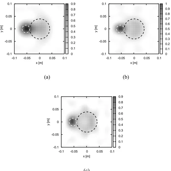
Figure 5 – Reconstructed distributions of the contrast function χ for different values of the frequency. (a) f = 2 GHz; (b) f = 3 GHz; (c) f = 4 GHz.

The results related to these data are reported in Figure 5. We notice that, even in this more complex configuration, the proposed simple method is able to obtain a quite good location and shaping of the two cylinders, at least for the three frequencies considered. Although a certain smoothing effect is present, it is worth noting that in all the three cases, the approach is quite able to correctly separate the cylinders.

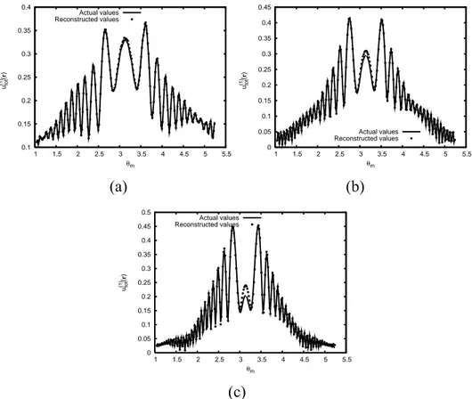
For completeness, Figure 6 gives the electric fields (measured and calculated values) at the measurement points for the first view and Figure 7 shows the error parameters γ and κ .

0.05 0.1 0.15 0.2 0.25 0.3 0.35 1 1.5 2 2.5 3 3.5 4 4.5 5 5.5 u (1)(tot r ) θm Actual values Reconstructed values 0 0.05 0.1 0.15 0.2 0.25 0.3 0.35 0.4 1 1.5 2 2.5 3 3.5 4 4.5 5 5.5 u (1)(tot r ) θm Actual values Reconstructed values (a) (b) 0 0.05 0.1 0.15 0.2 0.25 0.3 0.35 0.4 0.45 1 1.5 2 2.5 3 3.5 4 4.5 5 5.5 u (1) tot ( r ) θm Actual values Reconstructed values (c)

Figure 6 – Original and reconstructed electric fields (amplitude) at the measurement points for the first view. (a) f = 2 GHz; (b) f = 3 GHz; (c) f = 4 GHz.

0.65 0.7 0.75 0.8 0.85 0.9 0.95 1 0 5 10 15 20 γ Iteration number, j q = 1 q = 2 q = 3 0 0.5 1 1.5 2 2.5 3 3.5 0 5 10 15 20 κ Iteration number, j q = 1 q = 2 q = 3 (a) (b)

Figure 7 – Behavior of the error parameters γ (a) and κ (b) versus the outer iteration number, for different values of the frequency, fq = (q + 1)109 Hz.

4.3 Configuration (c) (FoamTwinDiel)

In the last considered case, the target object is a combination of the ones of the previous two configurations. There are two circular cylinders, and the first one (χ_obj1 =0.45) includes another

homogeneous circular cylinder with contrast function χ_obj2 =2. The two cross sections have diameters d_obj1 =0.08m and d_obj2 =0.03m, respectively, and they are centered in

m ) 0 . 0 , 0 . 0 ( 1 = obj

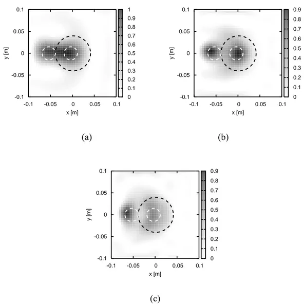
r and r_obj2 =(−0.005,0.0)m. The second cylinder, which is characterized by a diameter d_obj3 =0.03m and by a contrast function χ_obj3 =2, is located at r_obj3 =(−0.055,0.0)m. Figure 8 shows the recostructions obtained by using the proposed method. We can state that the results are good, although the accuracy in the shaping is worse than in the previous cases of configurations (a) and (b).

0 0.1 0.2 0.3 0.4 0.5 0.6 0.7 0.8 0.9 1 -0.1 -0.05 0 0.05 0.1 x [m] -0.1 -0.05 0 0.05 0.1 y [m] 0 0.1 0.2 0.3 0.4 0.5 0.6 0.7 0.8 0.9 -0.1 -0.05 0 0.05 0.1 x [m] -0.1 -0.05 0 0.05 0.1 y [m] (a) (b) 0 0.1 0.2 0.3 0.4 0.5 0.6 0.7 0.8 0.9 -0.1 -0.05 0 0.05 0.1 x [m] -0.1 -0.05 0 0.05 0.1 y [m] (c)

Figure 8 – Reconstructed distributions of the contrast function χ for different values of the frequency. (a) f = 2 GHz; (b) f = 3 GHz; (c) f = 4 GHz.

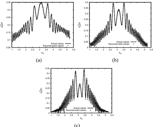
For this example, the values of the measured and reconstructed electric fields at the measurement points (first view) are reported in Figure 9. The figure shows that, for this configuration, only when f = 2 GHz and f = 3 GHz the proposed approach is able to approximate with good accuracy the

measured data. For f = 4 GHz, the fitting of the data is not as good as for the considered lower frequencies. 0.1 0.15 0.2 0.25 0.3 0.35 0.4 1 1.5 2 2.5 3 3.5 4 4.5 5 5.5 u (1) tot ( r ) θm Actual values Reconstructed values 0 0.05 0.1 0.15 0.2 0.25 0.3 0.35 0.4 0.45 1 1.5 2 2.5 3 3.5 4 4.5 5 5.5 u (1) tot ( r ) θm Actual values Reconstructed values (a) (b) 0 0.05 0.1 0.15 0.2 0.25 0.3 0.35 0.4 0.45 0.5 1 1.5 2 2.5 3 3.5 4 4.5 5 5.5 u (1) tot ( r ) θm Actual values Reconstructed values (c)

Figure 9 – Original and reconstructed electric fields (amplitude) at the measurement point for the first view. (a) f = 2 GHz; (b) f = 3 GHz; (c) f = 4 GHz.

This fact is also confirmed by Figure 10, which shows the error parameters γ and κ . For f = 4 GHz (q = 3), both the error on the reconstruction and the residual on the electric field data are higher than the ones obtained by using the lower frequencies. However, it should be noted that, for these "successful" lower frequencies, very few iterations are required to obtain a good solution with real input data starting from an empty domain.

0.7 0.75 0.8 0.85 0.9 0.95 1 1.05 0 5 10 15 20 γ Iteration number, j q = 1 q = 2 q = 3 0 1 2 3 4 5 6 0 5 10 15 20 κ Iteration number, j q = 1 q = 2 q = 3 (a) (b)

Figure 10 – Behavior of the error parameters (a) γ and (b) κ versus the outer iteration number, for different values of the frequency, fq = (q + 1)109 Hz.

4. Conclusions

In this paper, a new method for the reconstruction of dielectric cylinders has been validated by using experimental data. The approach is based on a two-step Inexact-Newton method applied to the Lippmann-Schwinger integral equation of the inverse scattering problem in the framework of the second-order Born approximation. Starting by initial solutions corresponding to completely empty test areas, the approach has shown excellent regularization capabilities in reconstructing separate and inhomogeneous dielectric cylinders. Although more sophisticated approaches can be applied, which are computationally much more expensive, in the authors' opinion the obtained reconstructions are quite interesting. In fact, despite a certain smoothing effects, the localization of the scatters is good and also the separation is acceptable for almost the considered configurations. In addition, the algorithm is simple to be implemented and seems to provide very good regularization and robustness features.

Acknowledgments

The authors would like to express their gratitude to M. Saillard and K. Belkebir, Institut Fresnel, Marseille, France, for providing the real scattered data and for the kind invitation to submit a contribution to the present special section.

References

[1] A. G. Tijhuis, K. Belkebir, A. C. S. Litman, and B. P. de Hon, Multiple-frequency distorted-wave Born approach to 2D inverse profilind, Inverse Problems, 17, 1635-1644.

[2] M. Miyakawa, K. Orikasa, M. Bertero, P. Boccacci, F. Conte, and M. Piana, 2002, Experimental validation of a linear model for data reduction in Chirp-Pulse microwave CT, IEEE Trans. Med. Im., 21, 385-395.

[3] B. Duchêne, 2001, Inversion of experimental data using linearized and binary specialized nonlinear inversion schemes, Inverse Problems, 17, 1623-1634.

[4] C. Dourthe, Ch. Pichot, J. Y. Dauvignac, and J. Cariou, 2000, Inversion algorithm and measurement system for microwave tomography of buried object, Radio Sci., 35, 1097-1108.

[5] C. Ramananjaona, M. Lambert, D. Lesselier, J. P. Zolésio, 2001, Shape reconstruction of buried obstacles by controlled evolution of a level set: from a min-max formulation to numerical

experimentation, Inverse Problems, 17, 1087-1111.

[6] T. J. Cui, A. A. Aydiner, W. C. Chew, D. L. Wright, and D. W. Smith, 2003, Three-dimensional imaging of buried object in very lossy earth by inversion of VETEM data, IEEE Trans. Geosci. Remote Sensing, 41, 2197-2209.

[7] G. Micolau, M. Saillard, and P. Borderies, 2003, DORT method as applied to ultrawideband signals for detection of buried objects, IEEE Trans. Geosci. Remote Sensing, 41, 1813-1820.

[8] S. Kent and T. Gunel, 1997, Dielectric permittivity estimation of cylindrical objects using genetic algorithm, J. Microwave Power and Electromagn. Energy, 32, 109-113.

[9] R. F. Bloemenkamo, A. Abubakar, and P. M. van den Berg, 2001, Inversion of experimental multi-frequency data using the contrast source inversion method, Inverse Problems, 17, 1611-1622. [10] O. Franza, N. Joachimowicz, and J.-C. Bolomey, 2002, SICS: A sensor interaction compensation scheme for microwave imaging, IEEE Trans. Antennas Propagat., 50, 211-216 [11] S. Caorsi, M. Donelli, A. Massa, M. Pastorino, 2004, Improved microwave imaging procedure for non-destructive evaluations of two-dimensional structures, IEEE Trans. Antennas Propagat., 52, 1386-1397.

[12] R. Azaro, G. Bozza, C. Estatico, A. Massa, M. Pastorino, D. Pregnolato, and A. Randazzo, "New results on electromagnetic imaging based on the inversion of measured scattered-field data," Proc. 2005 IEEE Instrum. Meas. Technol. Conf., special session on "Imaging Systems and Techniques", Ottawa, Ontario, Canada, 17-19 May 2005. In press.

[13] C. A. Balanis, Antenna Theory: Analysis and Design, New York, Wiley, 1982.

[14] M. Bertero and P. Boccacci, Introduction to Inverse Problems in Imaging, IOP, Bristol, UK, 1998.

[15] H. W. Engl, M. Hanke and A. Neubauer, Regularization of Inverse Problems, Kluver Academic Press, Dordrecht, 1996.

[16] H. W. Engl and P. Kugler, 2004, Nonlinear Inverse Problems: Theoretical Aspects and Some Industrial Applications, Multidisciplinary Methods for Analysis, Optimization and Control of Complex Systems, Series: Mathematics in Industry, Springer, 6, 3-48.

[17] M. Bertero, D. Bindi, P. Boccacci, M. Cattaneo, C. Eva, V. Lanza, 1997, Application of the projected Landweber method to the estimation of the source time function in seismology, Inverse Problems, 13, 465-486.

[18] M. Bertero, P. Boccacci, F. Di Benedetto and M. Robberto, 1999, Restoration of chopped and nodded images in infrared astronomy, Inverse Problems, 15, 345-372.

[19] R. Vio, J. Nagy, L. Tenorio and W. Wamsteker, 2004, A simple but efficient algorithm for multiple-image deblurring, Astron. Astrophys., 416, 403-410.