Neutronic analyses of the ALFRED LEADER core with deterministic (ECCO / ERANOS) and Monte Carlo (Serpent) codes: comparison between macroscopic-group constants, shutdown systems worth and spatial-angular flux distributions

(1)

(2)

1 Introduction

1.1 Aim and purposes

This technical report, produced in collaboration with Politecnico di Torino (PoliTO), represents

the first step of an ambitious work program whose final purpose is the production of the

homogenised and condensed multi-group cross-sections for the deterministic neutronic code

ERANOS [1] - usually produced with the ECCO cell code - through the Monte Carlo (MC) code

Serpent [2].

The motivation of this effort is twofold. In fact, with Serpent it is possible to model complex cell

geometries not reproducible by ECCO. Furthermore, the

Commissariat à l’énergie atomique et

aux énergies alternatives (CEA, France) decided to interrupt the ERANOS development and,

consequently, the updating process of the nuclear data evaluated in multi-group energy

structures suitable for the ECCO cell code [3]. The latest evaluated data available in ECCO

provided by the CEA are the JEFF-3.1 [4] and ENDF/B-VI.8 [5] libraries, actually rather dated.

The ECCO/ERANOS system has been widely used in ENEA for the core design and neutronic

analyses of fast reactors (e.g., Sodium Fast Reactors). In the last years, it has been adopted for

the design of the ALFRED (Advanced Lead Fast Reactor European Demonstrator) core, initially

conceived in the EURATOM FP7 LEADER (Lead-cooled European Advanced Demonstration

Reactor) project [6] and currently carried on within the FALCON (Fostering ALfred CONstruction)

international consortium [7]. The Lead-cooled Fast Reactor (LFR) concept - selected by the

Generation IV International Forum (GIF) [8] as one of the most promising nuclear systems for

the future - is nowadays widely investigated because it could effectively represent a viable

technology for safer, cleaner, cheaper and proliferation-resistant nuclear energy systems.

The ALFRED core design is challenging for the several technological constraints of the LFR

systems along with the target performances aimed for this demonstrator, such as [6]: the

maximum Pu enrichment (< 30%) in the Mixed OXide (MOX) fuel and the achievement of a peak

burn-up of 100 GWd/t, the narrow temperature range (400/480 °C as core inlet/outlet) and the

limiting temperature for the steel cladding in nominal conditions (550 °C

1

), the respect of the

system integrity even in extreme conditions, etc. Therefore, the design process requires many

scoping analyses, for which, relatively to neutronics, ERANOS is the main tool used in ENEA for

its flexibility and reduced computational times, especially in comparison with MC codes.

The ALFRED design defined in LEADER was used as reference for the present study, carried

out by adopting the JEFF-3.1 nuclear data library with both ECCO/ERANOS and Serpent codes.

The core models were accurately compared and their congruence verified in detail. The

comparison was limited to the Beginning of Life (BoL) conditions at full power (300 MW), with

fresh fuel and the shutdown systems completely withdrawn and inserted. The reference state is

represented by both shutdown systems withdrawn, which defines an over-critical core condition

at BoL: at the same time, this condition represents the easiest core configuration for a code

benchmark, since it does not involve the effects due the fuel burn-up and absorbers depletion.

A very detailed comparison between the deterministic and MC analyses was performed by

verifying (first of all) the full consistency between the two core models. This work summarises

the main outcomes of the study carried out in steady state, focusing on:



the macroscopic cross-sections produced by the ECCO and Serpent codes, whose

behaviour with respect to the incident neutron energy was accurately compared in all regions

of the core models. In general,

a good

agreement

between the two codes was found,

with

some noticeable exceptions (e.g., the absorbing bundles of the control and safety rods);

1

(6)



the different calculation options available in ECCO and Serpent, with the analyses of their

impact on the macroscopic-group constant values. In ECCO, the “reference” data were

obtained with 2D cell geometry models of the main core regions, an energy refinement at 33

groups (ECCO-33 grid) and the P

1

consistent approximation for the solution of the

multi-group transport equations. Additionally, the cross-sections were evaluated also with

homogeneous cell models, 80 energy groups and different calculation options (P

1

inconsistent, B

1

consistent and inconsistent and so on; see Appendix A). In Serpent all the

condensed and homogenised cross-sections were scored on the ECCO-33 grid using a 3D

Full-Core (FC) model (named MC1), a 2D radially-infinite model (named MC2) and, finally, a

3D axially-limited and radially-infinite model (named MC3) for the most important core

regions (e.g., fissile and absorbing parts of shutdown systems). The B

1

approximation was

used in order to provide leakage-corrected constants for the MC2 and MC3 cases;



the reactivity worth of the shutdown systems that differs by



10%, that is the usual

overestimation introduced by deterministic codes (with respect to stochastic ones) for fast

spectrum reactors as widely documented by the ENEA experience (e.g., [9]);



the impact of the shutdown systems insertion on the radial and axial spatial flux distribution

within the core. Besides the



10% reactivity worth difference, the flux spatial distributions

result sensibly different: both effects mainly derive from the different macroscopic-group

constants created by ECCO and Serpent for their absorbing regions. Additionally, the

different spatial distributions are necessarily related also with the different methods adopted

by deterministic and MC codes for the treatment of the flux angular dependency.

1.2 Organisation of the work

This report summarises part of the work carried out in collaboration between ENEA and PoliTO

in the last year dealing with the ALFRED core neutronic analyses with ECCO/ERANOS and

Serpent. It is structured as follows.



Chapter 2 describes briefly:

o the main features of the ALFRED core (in the LEADER version, §2.1);

o the core conditions examined (§2.2);

o the ERANOS model of the ALFRED core (§2.3).



Chapter 3 describes briefly:

o the ECCO/ERANOS system code (§3.1);

o

the procedure (“route”) adopted in ECCO to produce the reference data (i.e., multi-group

homogenised cross-sections representative of the core zones, §2.3), together with an

overview of the calculation options available whose theoretical background is described

in Appendix A; furthermore, their impact on the multi-group constant values evaluated at

the P

1

(and B

1

) order was accurately verified (§A.8).



Chapter 4 describes briefly:

o the Serpent MC code and the calculation options adopted to create the multi-group

homogenised cross-sections (§4.1);

o the Serpent model of the ALFRED core (§4.2).



Chapter 5 reports the most significant results of the cross-sections analyses and

comparison. While the full data set of the Serpent-ERANOS relative differences is reported in

Appendix B, in §5 are summarised:

o the most significant ECCO (§5.1) and Serpent (§5.2) cross-section results, together with

the impact of the different calculation options on their values;

(7)

o some significant comparisons between the ECCO and Serpent multi-group constants for

both fissile and non-multiplying media (§5.3 and §5.4, respectively);

o the main conclusions that can be drawn from the ECCO-Serpent comparison (§5.5).



Chapter 6 reports the most significant results of the ERANOS and Serpent full-core analyses

at BoL for what concerns the core reactivity, the shutdown systems performances and the

spatial distribution of the total flux within the core (with the control and safety rods completely

withdrawn and inserted). In particular:

o §6.1 reports the ERANOS values for the core reactivity and the shutdown systems worth.

The impact of the different ECCO calculation options was verified at the core level, as

well as the difference between the P

3

(reference) and P

1

flux order expansion in the

ERANOS spatial calculations;

o §6.2 reports the Serpent values for the core reactivity and the shutdown systems worth,

while §6.3 summarises some significant comparisons between the results of the two

codes;

o §6.4 reports the comparison between the radial and axial flux distributions within the core

obtained by ERANOS and Serpent with the shutdown systems fully withdrawn and

inserted. A couple of significant radial directions (passing through the core positions

hosting control and safety rods) were considered and their radial flux profiles compared,

as well as the axial ones for each assembly intercepted by these radial traverses. The full

data set of the axial flux traverses is reported in Appendix C.

Besides the most significant concluding remarks and future perspective of the present work (§7),

for the sake of completeness the report includes other two appendixes:



the ECCO/ERANOS input decks of the reference case, together with the indications of the

instructions to be modified to reproduce the different calculation options (Appendix D);



the Serpent code input decks used for the “reference” cross-sections generation and the

full-core analysis (Appendix E). Even in this case, the instructions to be modified and used to

explore the different calculation options are briefly provided. For more details about the code

calculation options, the reader is referred to the Serpent 2 code Wiki [10].

(8)

2 The ALFRED core design and conditions examined

2.1 Brief description of the ALFRED Leader core

Fig. 2.1 shows the main features of the MOX fuel pin (60 cm fissile length) and the wrapped

hexagonal Fuel Assembly (FA) made of 127 pins arranged in six rows of a triangular lattice. Fig.

2.2 shows a quarter of the core layout having a 90° symmetry, while Fig. 2.3 sketches the main

features of the shutdown systems design. The core layout is essentially made of [6]:



57 inner FAs and 114 outer FAs, having the same architecture but a different Pu enrichment

in the fuel pellet (21.7 and 27.8 at%, respectively) to flatten the core radial power distribution.

The fuel clad is made of 15-15/Ti austenitic Stainless Steel (SS) and the FA wrap is made of

T91 Ferritic Martensitic Steel (FMS);



12 Control Rods (CRs) located in the fuel outer zone, used for both normal control of the

reactor (i.e., start-up, reactivity control during the fuel cycle, power tuning and shutdown) and

for scram in case of emergency. In control mode, they partially enter the active region from

the bottom during irradiation (to compensate the initial over-criticality) and are progressively

withdrawn as far as the refuelling condition is reached (with an irradiation scheme made of 5

cycles of 1 year). The absorbing pin bundle is made of 19 pins embedding

Boron Carbide

(B

4

C) pellets

enriched at 90 at.% in

10

B. Inversely to the FA, the CR clads are made of T91

FMS and the surrounding tube is made of 15-15/Ti SS;



4 Safety Rods (SRs) located in the fuel inner zone, which stay still atop the active zone

during normal operation and, in emergency cases, enter the core by gravity for the reactor

shutdown. The SR bundle is made of 12 pins: as for the CRs, the absorber material is B

4

C

(with 90 at.%

10

B), the clad is in T91 FMS and the surrounding tube in 15-15/Ti SS;



the surrounding dummies, having the same structure of the FAs but with pins filled by

Yttria-stabilised Zirconia (YSZ) pellets (used also as axial thermal insulators in the fuel pin, see Fig.

2.1), acting as reflector for both neutron economy and shielding of the inner vessel.

(9)

Figure 2.2 ALFRED core layout [6].

Figure 2.3 ALFRED CR (left) and SR (right) design.

Both shutdown systems were similarly conceived (B

4

C pin bundles cooled by the primary lead,

see Fig. 2.3). The main difference (for the diversity requirement in case of scram) arises from

their mechanism of insertion relying on different physical phenomena.



The CRs’ fully withdrawn position is below the core: they are actuated by motors during

reactor operation, while for emergency shutdown they are provided with an electromagnetic

connection whose release allows for a rapid insertion into the core by buoyancy.



The SRs stay still atop the core in reactor operation and their actuation occurs only for scram

through the unlocking of an electromagnet. By the unlocking, the resistance to a pneumatic

system is simultaneously lost and the SRs are passively pushed rapidly into the core. To

face the failure of the pneumatic system, a tungsten ballast is added atop the SRs providing

a sufficient weight to counteract the buoyancy and ensuring their insertion into the core, even

if at a reduced speed.

(10)

2.2 Core conditions examined

The “reference” core models developed with ECCO/ERANOS (§3) and Serpent (§4) refer to the

full power (300 MW) conditions at BoL (i.e., fresh fuel everywhere) with the CRs completely

withdrawn 4 cm below the fissile zone and the SRs completely withdrawn 12 cm above it.

Therefore, the core examined is over-critical (i.e., the layout of 57 + 114 FA of Fig. 2.2 was

defined for the criticality at the equilibrium of the 5-year fuel cycle [6] and not at BoL when a

lower number of fresh FA will be loaded), but this over-critical condition does not represent a

limitation for the current study since the fundamental requirement for the neutronic codes

benchmark is the full consistency between the ERANOS and Serpent models, and the simplicity

of the model is preferred to avoid any influence of burnup modules on the actual benchmark.

In both codes, a cold geometry model (i.e., 20 °C) was considered while the nuclear data were

evaluated at the average working temperatures at full power reported in Table 2.1 for the fuel,

absorbers, structures and coolant. Differently from the solid materials, the coolant density was

correctly reproduced at its working temperature. As a main consequence, the fuel Doppler effect

is taken into account whereas the thermal dilatation of solid materials (e.g., fuel axial expansion)

is neglected. The main reason for this choice is due to the fact that Serpent is not endowed with

an ad hoc routine for the thermal dilatation as ECCO is, instead.

Besides the over-critical core model (i.e. full power BoL conditions with CRs and SRs completely

withdrawn, representing the simplest configuration to be simulated), the calculations with both

codes were extended to include the case of complete insertion of the shutdown systems, in

order to compare their reactivity worth values. The complete withdrawn and fully inserted

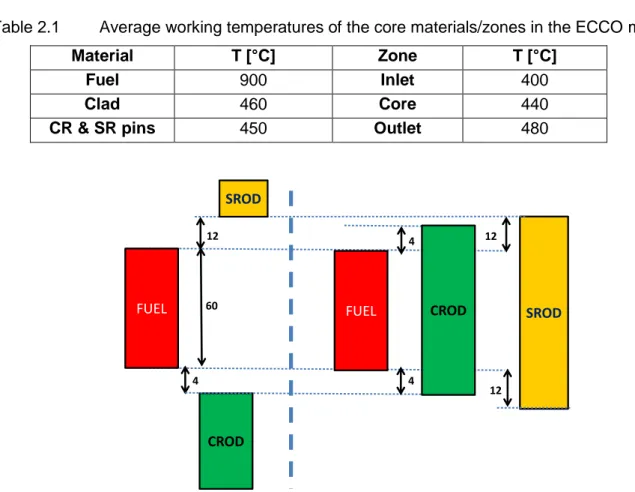
positions are sketched in Fig. 2.4 for both systems, where

“CROD” and “SROD” are the

absorbing bundles of the CRs and SRs, respectively (see also Fig. 2.5).

Table 2.1

Average working temperatures of the core materials/zones in the ECCO model.

Material

T [°C]

Zone

T [°C]

Fuel

900 Inlet

400 Clad

460 Core

440 CR & SR pins

450 Outlet

480 Figure 2.4 ALFRED CRs’ and SRs’ absorbing bundle positions when fully withdrawn (left)

and inserted (right; figure not in scale, dimensions in cm).

FUEL

12 FUEL

_SROD

12

4 CROD

12 SROD

60

4 CROD

4

(11)

2.3 The ALFRED core model with ECCO/ERANOS

Fig. 2.5 depicts the ERANOS axial model of the core assemblies (FA, CR, SR and dummy,

§2.1). All the axial zones (i.e., hexagonal slices of a certain thickness) of these elements were

characterised with the ECCO cell code to obtain the corresponding (homogeneous equivalent)

macroscopic cross-sections. A list of all the zones - together with their brief description and

acronyms used in Fig. 2.5 - is provided in the following.



In the FA (see also Fig. 2.1): the bottom reflector (BREF), the bottom plug of the fuel pins

(BPLG), the plenum (PLEN, i.e., voided pin clads containing a thin cylindrical tube in 15-15/Ti

SS as support for the fuel pellets), the bottom thermal insulator (BINS, i.e., pin clads filled

with YSZ pellets), the fissile zone (FINN and FOUT for the inner and outer FA, respectively),

the top insulator (TINS), the spring (SPRN, i.e., plena with a 15-15/Ti SS spring), the top plug

(TPLG) and the top reflector (TREF).



In the dummy: the reflector region (DUMM) that is identical to the BINS and TINS ones. It is

however necessary to evaluate different cross-sections to take into account their different

temperatures in operating conditions (see Table 2.1). The other zones (below and above the

DUMM region) are identical to the FA ones.



In the CR: the absorbing part (CROD, made of B

4

C pellets in T91 FMS clads) and its follower

(FROD, i.e., clads with YSZ pellets). For the sake of simplicity, the other zones were

assumed identical to the FA ones in order to have a unique data set of cross-sections

2

.

Nevertheless, such approximation is acceptable since it does not introduce significant biases

in the resulting cross-sections, as well as in the full-core features here examined (i.e., core

reactivity, flux distributions, CRs and SRs reactivity worth).



In the SR: the absorbing part (SROD) made of B

4

C pellets in T91 FMS clads as the CR but

with different dimensions (resulting in a lower B

4

C volume fraction; see Fig. 2.3). As for the

CR, the other zones were assumed identical to the FA ones to simplify the core modelling

without penalising the calculations accuracy.

All the core regions shown Fig. 2.5 were modelled with ECCO by adopting a 2D heterogeneous

geometry, with the exception of the axial reflectors (BREF and TREF), the external lead in the

down-comer (Ext Pb), the inner vessel and the surrounding lead, which were described with

homogeneous models. Table 2.2 reports the materials volume fractions in them with the density

values representing the materials mix. The densities of the solid ones were considered at room

temperature, while the lead density values were obtained from an extrapolation of its linear

behaviour with temperature in the liquid phase [11] down to 20 °C. The inner vessel (or barrel

made of 316L SS) was modelled with 72 assemblies, which represent a homogeneous mix of

steel and lead to simulate it and the surrounding coolant in a hexagonal position of the core

lattice. Other rings of “virtual” assemblies made by lead only were introduced in the ERANOS 3D

hexagonal core model to simulate the down-comer outside the inner vessel.

Due to the ECCO cell code limitations, the CR and SR bundles (Fig. 2.3) were modelled as the

FA, with the pins arranged in triangular lattices (by preserving the materials volume fractions)

and the surrounding SS tube described with a hexagonal wrap having an equivalent volume.

Table 2.3 reports the materials density (at 20°C), their volume fraction in the FA, CR, SR and

dummy clads, and the corresponding filling densities. The MOX density is computed from the

theoretical one by assuming a 5% porosity. The filling density represents the “effective” density

of the materials (MOX, YSZ, B

4

C and 15-15/Ti SS) diluted in the corresponding clads. This

dilution is usually adopted in deterministic codes because of their difficulty in simulating regions

with “voids” or with materials having a very low density, such as the gap between fuel pellets and

clads filled by He gas [6].

2

As an example, the material/geometrical features of the SPRN zone of the FA were assumed also for the

SPRN regions of the CR and SR.

(12)

Figure 2.5

The ERANOS axial model of the ALFRED core assemblies (not in scale).

CR IN CR Out SR IN SR Out

Compl. In Compl. Out Compl. In Compl. Out

340 340TREF 8 340 340 340 33 340 332 332 307 307 SPRN 10 297 297 TINS 1 296 296 272 272 264 264 223 223 218 218 213 213 TINS 1 213 212 212 212 207 207 204 204 204 201 TINS 1 201 200 140 BINS 1 139 136 136 BINS 1 136 135 135 _BPLG ₅ 130 130 128 128 123 123 84BPLG 5 84BPLG 5 79 79 68 68 BINS 1 67 67 BPLG 5 62 62 BREF CROD FROD SPRN 60 68 68 130 76 62 68 SPRN 84 5.0 207 5 12 117 79 BREF DUMM SPRN TPLG h [cm] Dummy h [cm] TREF 60 TREF SPRN SROD BPLG BREF 123 5 84 10 117 12 FROD 68 TREF 122 SPRN TREF BREF 79 CROD PLEN 55 TREF 122 h [cm] FA h [cm] h [cm] h [cm] TPLG 5 FUEL 60 BREF BREF BPLG SROD

(13)

Table 2.2

ECCO models of homogeneous core zones: materials volume fraction and

density (at 20°C).

Zone

15-15/Ti SS

[vol. %]

Pb

[vol. %]

Density**

[g cm

-3

]

BREF

12.0

88.0

10.649 TREF

20.0

80.0

10.404 Barrel*

33.8

66.2

9.980 Ext Pb

100.0

11.017 * actually, the ECCO cell for the barrel is made of 316L SS (instead of 15-15/Ti) and surrounding coolant

** of the materials mix

Table 2.3

Materials density (at 20°C) and their corresponding filling density in the FA, CR,

SR and dummy clads.

Material

Density

ZONE

Fraction in

clad [vol. %]

Filling density

in clad [g cm

-3

]

[g cm

-3

]

MOX (FINN)

10.494 FINN

89.028 9.3426

MOX (FOUT)

10.513 FOUT

89.028 9.3595

YSZ

6.0 BINS, TINS, DUMM

93.652 5.6191

FROD

94.703 5.6822

15-15/Ti SS

7.95 PLEN

7.559**

0.6009**

SPRN

7.594 0.6037

B

4

C

2.2 CROD, SROD

94.703 2.0835

FMS T91

7.736 FA wrap, CR and SR tubes*

Pb

11.017 Everywhere

* modelled as equivalent hexagonal layers

(14)

3 The ECCO/ERANOS system code

3.1 Brief description of the ECCO/ERANOS system code

The European Reactor ANalysis Optimised System (ERANOS) was developed by CEA for the

core design of Sodium Fast Reactors [1]. It is a modular system and consists of data libraries,

deterministic codes and calculation procedures: the different modules perform several functions

to analyse the core reactivity, flux distributions, burn-up and reaction rates, etc. of a nuclear

system that can be modelled by 1D, 2D and 3D geometries. The cross-sections of the core

regions are usually produced in a 1968 energy-group structure and condensed to the standard

one at few groups (e.g., 33) by the European Cell COde (ECCO) [3].

The ERANOS system code has been widely used by ENEA in the last 20 years for the core

design of the LFR and Accelerator Driven Systems, e.g. [9], [12] and [13]. As mentioned in §1,

the nuclear data suitable for ECCO in different energy structures are based on evaluated data:

specifically, the JEFF-3.1 library [4] was adopted in this study. The multi-group macroscopic

cross-sections (or macroscopic-group constants) obtained by ECCO are then used for the

ERANOS full-core calculations. In the 3D hexagonal geometry model of the ALFRED core, they

were carried out with the TGV module [14] adopting the variational-nodal method [15, 16].

Since the ECCO cell code was developed for the analysis of fast reactors, it considers correctly

the peculiarities of this kind of systems like the neutron slowing down, the self-shielding effect,

the inelastic and/or non-isotropic scattering events, etc. In the “reference” cell calculation option,

a 2D heterogeneous geometry model was adopted to reproduce the spatial self-shielding effect

(§2.3) and approached with the collision probability method for the flux solution [3] to take into

account the cells heterogeneity. Successively, the cross-sections were homogenised (with the

flux times volume weighting method) to obtain homogeneous equivalent values to consider (at

some extent) the heterogeneity of the cell.

3.2 The ECCO calculation reference route

The ECCO model of the ALFRED core assemblies (Fig. 2.5) relies on an accurate 2D geometry

description of them [17], while the axial leakages were taken into account by tuning opportunely

the buckling value (identical for each energy group). More specifically [3]:



in the fissile zone of the FA, the bucking value is calculated by ECCO in order to yield a

unitary multiplication factor (k

eff

) so as to reproduce the critical core condition;



in the non-fissile zones the ECCO calculation procedures foresee the introduction of an

external source, having the (flux and current) spectrum of the (nearest) fissile region and

uniformly distributed in space within the zone. The bucking value is fixed by a semi-empirical

relation depending on the (radial or axial) thickness of the zone examined (see Appendix A).

The method recommended by the ECCO developers - called reference route [3] - was used to

create the macroscopic cross-sections of the core regions. Fig. 3.1 summarises this route, which

foresees at least four steps in which the calculations:



start with a homogeneous geometry description of the cell and a broad energy structure,

usually at 172 or 33 groups (172 were chosen as reference);



introduce the heterogeneous geometry description of the cell by maintaining the broad

energy structure;



refine the energy grid at 1968 groups for the nuclides included in the evaluated library (the

most important ones for ALFRED are available) by maintaining the heterogeneous model;



end with the spatial homogenisation of the cell and the energy collapsing in a broad energy

structure at 33 groups. For the codes benchmark, the same energy grid was adopted to

create the cross-sections with Serpent (§4).

(15)

Figure 3.1 Reference route for the ECCO calculations [3].

As a net result, the macroscopic cross-section “x” (x=total, fission, capture, elastic, inelastic, etc.)

was evaluated at the P

1

order of the transport equation in a broad energy-group-structure:

(3.1)

where:



“g” (1-33) is the energy (E) group considered;



the neutron flux “

ϕ(𝐫, E)

” is used as weighting function in the integrals, in order to keep the

reaction rates constant e.g., during the condensation process from 1968 down to 33 groups;



“r” is the position within the cell and, trivially, the final homogeneous equivalent values of the

macroscopic cross-sections obtained by integrating over the volume “V” do not vary with r.

The multi-group constants of the non-fissile zones modelled by a heterogeneous geometry in

ECCO (see §2.3) were obtained with the four-step calculation procedure of Fig. 3.1 and are

usually named Heterogeneous Homogenised (HH) cross-sections (



HH

). For the fissile zones,

the last step was divided in two by treating the energy collapsing and the spatial homogenisation

separately. An additional sixth step can be added by imposing the buckling at zero, in order to

make the leakage term vanish and to evaluate the k-infinite (k

inf

) parameter of the fuel cells.

The mathematical basis of the ECCO cell analyses - producing the macroscopic cross-sections

(vectors and matrices) for ERANOS - is described in detail in Appendix A, together with the

different calculation methodologies adopted. The cross-section behaviours with energy produced

by the different ECCO methods were compared, as well as their impact on the main ERANOS

full-core quantities. The ECCO calculation options examined in this work deal with:



the initial energy refinement, i.e., by starting with 33 energy groups (instead of 172) for both

fissile and non-fissile zones;



the final energy refinement, i.e., by a final collapsing in a structure at 80 groups (instead of

33) for both fissile and non-fissile zones;

HOM geometry

172 E groups

HET geometry

172 E groups

HET geometry

1968 E groups

HOM geometry

33 E groups

𝛴

_𝑥,𝑔

=

∫ ∫

ϕ(𝐫, E)Σ

x

(𝐫, E)dE

𝐸𝑔+1

Eg

𝑉

∫ ∫

_𝑉

_Eg

𝐸𝑔+1

ϕ(𝐫, E)dE

(16)



the homogeneous geometry models of the ECCO cells describing the fissile zone of the FA

and the absorbing regions of shutdown systems, which are the most important zones for

neutronics;



the adoption of the (flux and current) fuel spectrum generated by Serpent (at 33 energy

groups) as weighting function in Eq. (3.1) to obtain the HH cross-sections for the

non-multiplying media. The Serpent fuel spectrum was introduced as an “external source” in

ECCO and, to verify the congruence of this calculation option, the same method was used

also by inserting “externally” the “internal” spectrum evaluated by ECCO itself.

The macroscopic cross-sections were created with a 33-group structure (the reference one, see

Table 3.1 reporting its upper energy limits) and the more refined one at 80 groups (see Table

3.2). The latter reports in the last column also the upper energy limits in correspondence with the

structure at 1968 groups (to be used in the ECCO CONDENSE instruction; see Appendix D).

Table 3.1

The 33-energy-group structure (Group / Energy [MeV]).

1 1.9640E+01

2 1.0000E+01

3 6.0653E+00

4 3.6788E+00

5 2.2313E+00

6 1.3534E+00

7 8.2085E-01

8 4.9787E-01

9 3.0197E-01

10 1.8316E-01

11 1.1109E-01

12 6.7380E-02

13 4.0868E-02

14 2.4788E-02

15 1.5034E-02

16 9.1188E-03

17 5.5308E-03

18 3.3546E-03

19 2.0347E-03

20 1.2341E-03

21 7.4852E-04

22 4.5400E-04

23 3.0433E-04

24 1.4863E-04

25 9.1661E-05

26 6.7904E-05

27 4.0169E-05

28 2.2603E-05

29 1.3710E-05

30 8.3153E-06

31 4.0000E-06

32 5.4000E-07

33 1.0000E-07

(17)

Table 3.2

The 80-energy-group structure (Group / Energy [MeV] / Group in 1968 grid).

1 1.9640E+07

1

2 1.6905E+07

19

3 1.4918E+07

34

4 1.3499E+07

46

5 1.1912E+07

61

6 1.0000E+07

82

7 7.7880E+06

112

8 6.0653E+06

142

9 4.7237E+06

172

10 3.6788E+06

202

11 2.8650E+06

232

12 2.2313E+06

262

13 1.7377E+06

292

14 1.3534E+06

322

15 1.1943E+06

337

16 1.0540E+06

352

17 9.3014E+05

367

18 8.2085E+05

382

19 7.2440E+05

397

20 6.3928E+05

412

21 5.6416E+05

427

22 4.9787E+05

442

23 4.3937E+05

457

24 3.8774E+05

472

25 3.0197E+05

502

26 2.3518E+05

534

27 1.8316E+05

564

28 1.4264E+05

594

29 1.1109E+05

624

30 8.6517E+04

654

31 6.7379E+04

686

32 5.2475E+04

716

33 4.0868E+04

746

34 3.1828E+04

776

35 2.8088E+04

792

36 2.6058E+04

802

37 2.4788E+04

808

38 2.1875E+04

823

39 1.9305E+04

838

40 1.7036E+04

853

41 1.5034E+04

868

42 1.3268E+04

883

43 1.1709E+04

898

44 1.0333E+04

913

45 9.1188E+03

928

46 8.0473E+03

943

47 7.1017E+03

958

48 6.2673E+03

973

(18)

49 5.5308E+03

988

50 4.8810E+03

1003

51 4.3074E+03

1018

52 3.8013E+03

1033

53 3.3546E+03

1048

54 2.9604E+03

1063

55 2.6126E+03

1078

56 2.3056E+03

1093

57 2.0347E+03

1108

58 1.7956E+03

1123

59 1.5846E+03

1138

60 1.3984E+03

1153

61 1.2341E+03

1168

62 1.0891E+03

1183

63 9.6112E+02

1198

64 7.4852E+02

1228

65 5.8295E+02

1258

66 4.5400E+02

1288

67 3.5358E+02

1318

68 2.7536E+02

1348

69 1.6702E+02

1408

70 1.0130E+02

1468

71 6.1442E+01

1528

72 3.7267E+01

1588

73 2.2603E+01

1648

74 1.3710E+01

1708

75 8.3153E+00

1768

76 5.0435E+00

1828

77 3.0590E+00

1848

78 1.1230E+00

1892

79 4.1399E-01

1927

80 1.5303E-01

1947

(19)

4 The SERPENT code and its ALFRED core model

4.1 Brief description of the SERPENT code

Serpent ([2], [10], and [18]) is a MC code written in C language and developed at VTT Technical

Research Centre of Finland. Its original purpose was to fill the gap left by MCNP (developed by

LANL [19]) for the multi-group cross-section energy collapsing and spatial homogenisation.

Since 2004, both the code capabilities and its user community have steadily grown, and

nowadays Serpent is a reference tool for fission reactor physics research and development. With

the latest code version (2.1.31), the users can now perform: cross-section homogenisation at the

assembly level, burn-up calculations, coupled neutron-photon transport calculations, uncertainty

evaluation and multi-physics simulations in coupling with the OpenFOAM toolbox [20].

The spatial homogenisation of the multi-group constants can be carried out in many ways.

Thanks to the code flexibility, the user can decide to collapse the constants over arbitrary energy

grids and to compute them for different reactor regions without too much effort.

Serpent 2 employs a 3D Constructive Solid Geometry (CSG) routine which enables the user to

easily nest different universes (i.e., sets of surfaces and cells for a detailed representation of

each reactor spatial scale, from the fuel pin up to the FA/core level). This routine can thus be

used to generate both 3D objects and 2D systems, like the traditional cells defined for lattice

calculations. According to the geometrical model adopted, the stochastic transport of neutrons

inside the core may require very different computational times as well as it can provide different

levels of statistical accuracy.

Once the system is geometrically defined, the code reads the continuous-energy data

(cross-sections, angular distributions, fission emission spectra, and so on) from the selected nuclear

data library and evaluates them over a unionized energy grid, in order to reduce the memory

consumption. After these preliminary steps, the code performs a bunch of “inactive” cycles in

order to initialise the fission source

3

. At the end of the inactive cycles, the statistical scoring

begins.

The effective HH cross-section for a certain reaction “x” over a group “g” is usually evaluate

preserving the associated reaction rate:

Σ

𝑥,𝑔

=

⟨Σ

𝑥

(𝒓, 𝐸)|𝜙(𝒓, 𝐸)⟩

𝑉,𝑔

〈𝜙(𝒓, 𝐸)〉

𝑉,𝑔

(4.1)

where the bracket notation indicates an integration over the volume “V” for each energy group

“g”, while the other variables have the usual meaning (see §3.2).

While deterministic codes usually rely on application data libraries evaluated on a limited number

of groups (e.g., 33, 172, 175 and 1968 in ECCO), MC codes allow reading the

continuous-energy data, avoiding any data pre-processing. Thanks to this continuous-energy management, Serpent 2

implicitly takes into account all the self-shielding effects, without any approximation. In addition,

also the unresolved resonance region is treated more accurately, as the user can force the code

to sample the data from the probability tables (the so-called p-table) in the A Compact ENDF

(ACE) format specification files [21]. This option (available also in ECCO in a multi-energy-group

form; §3.1) is particularly important for fast systems, where the flux in the unresolved resonance

region assumes relevant values.

Another significant difference with respect to the ECCO cell code is the number of steps

employed to evaluate equation (4.1) (identical to (3.1)). If the reference calculation route is

3

In each cycle, a certain number of neutron histories is simulated: once the initial position, energy and

flying direction of a particle are sampled, the particle starts moving and colliding with the medium, and its

history ends when the particle leaks from the domain or it is absorbed.

(20)

employed, ECCO computes the integral in 4-5 steps (§3.2) while Serpent 2 firstly evaluates the

effective cross-section on an intermediate group structure called fine grid (the WIMS-69 grid is

the default choice, but the user can change it) and then it condenses the Σ

_𝑥

over the few-group

grid required by the user (33 in this study; see Table 3.1). If the number of energy groups

required is larger than 69 (as for the 80 groups case, see Table 3.2), the fine grid coincides with

the few-group grid.

The reason for this two-steps calculation is simplifying the implementation of the spatial

homogenisation, which can be carried out by the code in two ways: the infinite-lattice procedure,

which is always performed, and the leakage-corrected calculation, that has to be switched on by

the user. The first routine does not introduce any correction to the code output, which thus

strongly depends on the flux distribution in the geometry considered, while the leakage-corrected

mode, known as B

1

calculation, applies a correction that takes into account the fact that the cells

defined are usually sub- or super-critical. The main hypotheses made in Serpent 2 are that the

flux can be factorised in angle, space and energy, so that an eigenvalue problem for the material

buckling can be retrieved. This problem is solved iteratively until a spatial buckling providing a

critical system is reached. The fundamental eigenfunction found to solve this problem is then

employed to collapse the effective constants over the few-group structure instead of the

non-corrected flux. Since the homogenisation is performed in two steps, the B

1

calculation mode

does not take full advantage of the continuous-energy MC capabilities, as the leakage-corrected

flux is evaluated over the few-group grid. Thanks to the options available in the code, however,

the user can make the few-group and the fine-group structures overlap, to minimise the

condensation errors.

The other, straightforward face of the medal is that Serpent, as an MC code, is affected by the

statistical noise of its results, which – although subject to due management by the experienced

user, to the price of increasing the computational burden – is inherent to its stochastic nature.

4.2 The Serpent models of the ALFRED core and calculation options adopted

T

he Serpent core model is based on the ERANOS one described in §2.2 (see Figs. 2.3 and 2.5)

and it is shown in Figs 4.1 and 4.2.

As mentioned in §4.1, the quality of the (leakage) non-corrected calculation, which is the default

one, improves with the reactor geometrical model: therefore, the most accurate set of

multi-group constants would be evaluated scoring them over each assembly family with a 3D FC

model, since the flux used to weight the cross-sections would be the most representative of a

certain core region. However, the computational time of a full-core calculation would be too

much for design calculation purposes. On the other hand, cell calculations, that are radially and

axially infinite thanks to the reflective boundary conditions, are suitable for design but the results

quality suffers from the geometrical simplification. This issue can be tackled for multiplying

regions employing a B

1

calculation, but an alternative treatment for inactive regions like CRs,

SRs or dummy reflector assemblies is needed.

The most intuitive option would be to simulate a mini-core made of one or more non-fissile

assemblies in the centre (for which the homogenised and collapsed data are desired)

surrounded by some rings of FA. This solution, however, would require a criticality calculation for

each different inactive region, making the computational time comparable with the one of a FC

calculation but much less accurate. Moreover, sensitivity studies would be required to assess

the impact of the number of assemblies for both the active and inactive regions on the overall

leakage effect.

To preserve the cell calculation main features (i.e., a good compromise between computational

speed and accuracy) also for non-fissile assemblies and, at the same time, to properly consider

the leakage effects, the following strategy has been devised. The inactive region is studied

(21)

considering an isotropic source of particles with the same energy spectrum of the fuel and

spatially distributed across a radially infinite cell with finite height, equal to the active height of

the fuel rods. Since this approach can induce strong modifications in the flux energy spectrum

due to the absence of the axial reflectors, the cell was surrounded by a top and a bottom layer of

lead. This precaution allows obtaining a flux which is closer to the physical one and, at the same

time, to increase the statistics of the groups at the lowest energies.

To sum up, the following models have been employed by Serpent (used as a cell code; §3) to

carry out the spatial homogenisation and the energy collapsing.

1. The 3D FC heterogeneous model (see Fig. 4.1) with homogeneous core assemblies (FA,

CR, SR, dummy) and barrel (SS and lead homogenised over a hexagonal area; see §2.3).

Outside an external lead layer surrounding the barrel, void boundary conditions are imposed.

2. The most accurate 3D FC heterogeneous model with heterogeneous core assemblies (only

the barrel and external lead were assumed homogeneous; see Fig. 4.2). Outside the

external lead layer, void boundary conditions are imposed.

3. The 3D axially and radially infinite cells with heterogeneous core assemblies (see Fig. 4.3),

with the B

1

calculation mode for FA and the source calculation one for non-fissile regions.

The “cell” is built with a limited number of assemblies, but the imposition of reflective

boundary conditions forces the particles to move in the system as if it were infinite.

4. The 3D radially infinite but axially finite cells with homogeneous core assemblies (see Fig.

4.4), with the B

1

calculation mode for FA and the source calculation one for non-fissile

regions. The void boundary conditions are imposed axially, while reflective conditions are set

radially.

5. The 3D radially infinite but axially finite cell with heterogeneous core assemblies (see Fig.

4.5), with the B

1

calculation mode for FA and the source calculation one for non-fissile zones.

As before, void and reflective boundary conditions were settled axially and radially,

respectively.

(22)

Figure 4.2 The 3D FC model with heterogeneous core assemblies (reference).

Figure 4.3 Axially and radially infinite model with heterogeneous assembly geometries.

Figure 4.4 Axially finite and radially infinite model with homogeneous assembly geometries.

Figure 4.5 Axially finite and radially infinite cell model with heterogeneous assembly

geometries.

(23)

The first model, in which the core assemblies are assumed to be spatially homogeneous (see

Fig. 4.1), is an approximation of the second one (see Fig. 4.2), which can be assumed as a

reference since it accurately represents the whole ALFRED core geometry. The other three

models are the closest to the ECCO ones, since they represent a single region within a cell.

However, there are some intrinsic differences between the stochastic and the deterministic

approaches for cell calculations, in addition to the ones already mentioned.

The first difference is due to the neutron spectrum. In a fast reactor, the particles mean free path

is longer than in moderated systems: therefore, in principle the cell dimensions can have a

detrimental effect on the cross-sections accuracy, as the reflective boundary conditions would

force the particles to collide within the cell itself, increasing artificially the reaction rate inside the

region. However, since the ALFRED core composition can be roughly divided into three rings

characterised by the same kind of assemblies (inner fuel, outer fuel and dummy elements), the

error induced by considering an infinite cell is negligible, as shown in the results section (§5.2).

The second difference between deterministic and stochastic cell calculations is related to

statistics. Since the presence of thermal particles inside the FA cell of a fast reactor is a rare

event, the statistical error on the effective cross-sections can be significantly high at low

energies. In principle there are many ways to reduce the statistical noise, like simulating a huge

number of particles or employing some variance reduction techniques. However, the first

approach could increase too much the computational time for design-oriented calculations, while

the second is currently not possible in Serpent 2, as there are no variance reduction techniques

available in the cross-sections generation based on flux-engeinvalue calculations. An alternative

strategy could be “helping” the thermal population to increase, surrounding the cells axially with

a layer of lead, so that more particles are slowed down and reflected back into the cell. This

approach (i.e., simulating an axially limited cell) would change the cell spectrum making it closer

to the one of the FC (where the presence of the axial reflectors and of the other components,

like pin insulators and plugs, softens the flux spectrum) by enhancing the calculation accuracy of

its thermal component.

(24)

5 Comparison between ECCO and SERPENT cross-sections data

5.1 The most significant ECCO multi-group cross-section results

The macroscopic cross-section vectors (3.1) representing the most significant core zones are

reported in the following graphs. They were obtained by ECCO at 33 energy groups by adopting

the reference route described in §3.2 (and explained in more detail in §A.8). Fig. 5.1 shows the

main cross-section results for the fuel inner (top) and outer (bottom) zones. It is evident that the

elastic, capture and fission values are dominant over the whole spectrum, with the exception of

the inelastic and (n,xn) threshold reactions above 0.1 and 2 MeV, respectively. Fig. 5.2 shows

the CR (top) and SR (bottom) absorbing bundle (B

4

C) cross-sections: the elastic and capture

values are dominant over the whole spectrum, with the exception of the inelastic and (n,xn)

threshold reactions at high energies.

Figure 5.1 Fuel inner (top) and outer (bottom) macroscopic cross-sections

(ECCO results: P

1

order, heterogeneous geometry, 33 energy groups).

1.E-06

1.E-05

1.E-04

1.E-03

1.E-02

1.E-01

1.E+00

1.E+01

1.E-07

1.E-06

1.E-05

1.E-04

1.E-03

1.E-02

1.E-01

1.E+00

1.E+01

1.E+02

cm

-1

MeV

FA Inner

Total

Capture

Elastic

Inelastic

n,xn

Fission

1.E-06

1.E-05

1.E-04

1.E-03

1.E-02

1.E-01

1.E+00

1.E+01

1.E-07

1.E-06

1.E-05

1.E-04

1.E-03

1.E-02

1.E-01

1.E+00

1.E+01

1.E+02

cm

-1

MeV

FA Outer

Total

Capture

Elastic

Inelastic

n,xn

Fission

(25)

Figure 5.2 CR (top) and SR (bottom) absorbing bundles macroscopic cross-sections

(ECCO results: P

1

order, heterogeneous geometry, 33 energy groups).

Fig. 5.3 shows the FA plena (left) and the pure lead (external to the barrel; right) cross-sections:

it is evident that the elastic values are dominant over the whole spectrum, with the exception of

the inelastic and (n,xn) threshold reactions at high energies.

Figure 5.3 FA plena (left) and pure lead (right) macroscopic cross-sections

(ECCO results: P

1

order, 33 energy groups).

1.E-06

1.E-05

1.E-04

1.E-03

1.E-02

1.E-01

1.E+00

1.E-07

1.E-06

1.E-05

1.E-04

1.E-03

1.E-02

1.E-01

1.E+00

1.E+01

1.E+02

cm

-1

MeV

CR B

₄

C bundle

Total

Capture

Elastic

Inelastic

n,xn

1.E-06

1.E-05

1.E-04

1.E-03

1.E-02

1.E-01

1.E+00

1.E-07

1.E-06

1.E-05

1.E-04

1.E-03

1.E-02

1.E-01

1.E+00

1.E+01

1.E+02

cm

-1

MeV

SR B

₄

C Bundle

Total

Capture

Elastic

Inelastic

n,xn

1.E-06 1.E-05 1.E-04 1.E-03 1.E-02 1.E-01 1.E+00

1.E-07 1.E-06 1.E-05 1.E-04 1.E-03 1.E-02 1.E-01 1.E+00 1.E+01 1.E+02

cm-1 MeV

Plenum (FA)

Total Capture Elastic Inelastic n,xn 1.E-07 1.E-06 1.E-05 1.E-04 1.E-03 1.E-02 1.E-01 1.E+00

1.E-07 1.E-06 1.E-05 1.E-04 1.E-03 1.E-02 1.E-01 1.E+00 1.E+01 1.E+02 cm-1 MeV

Pure lead

Total Capture Elastic Inelastic n,xn

(26)

5.2 Impact of different SERPENT models on multi-group cross-sections

This section reports some comparisons between the ECCO “reference” multi-group constants at

33 energy groups (§3.2) and the Serpent ones in the same energy grid obtained with different

geometrical models and calculation options (§4.2). The results here reported are the most

interesting and relevant ones obtained in this study. The analysis concerned mainly the transport

cross-section (which is directly linked to the diffusion coefficient), the capture and the fission

cross-sections. The scattering matrix comparison has been left for future evaluations.

While the multi-group constants reported in Figs. 5.1-5.3 are depicted in their “correct” histogram

form, for easiness in the following graphs they are reported in a “punctual form” (with the

multigroup cross-section values in correspondence of the upper energy limits) as they come out

from the codes output. The complete set of the relative differences between the ECCO and

Serpent cross-section results at 33 groups is reported in Appendix B.

5.2.1 Main comparisons for multi-group constants of fissile zones

Figs. 5.4, 5.5 and 5.6 show the transport, capture and fission cross-sections, respectively,

scored on the ECCO-33 energy grid, for the inner fuel region. In all the three graphs, the lowest

energy point in the green curve (Serpent B

1

option with a heterogeneous 3D cell axially infinite)

is missing because of poor statistics.

An inspection of the data represented in these plots suggests that the Serpent models that

provide the closest results to the ECCO “reference” HH cross-sections (light blue curve, §3.2)

are the 3D FC and the axially limited infinite cell models (brown and purple curves, respectively),

where both the inner and outer fuel regions are considered as spatially homogeneous.

The multi-group constants evaluated with Serpent usually come out with a Relative Standard

Deviation (RSD) less than 1%, by the exception of the spectrum tails (first thermal and last fast

groups, respectively), where it can reach values up to 30%.

For energies above 100 eV there is a good general agreement between the two codes with a

relative error approximately below 10%, while at lower energies significant discrepancies (that

can reach even 100% in the thermal region) appear. These larger differences are mainly due to

Serpent statistical noise at low energies. Similar trends can be found also for the outer fuel

region: they were omitted for the sake of conciseness.

Figure 5.4 Transport macroscopic cross-sections at 33 energy groups of the inner fuel with

the ECCO “reference” and different Serpent models.

(27)

Figure 5.5 Capture macroscopic cross-sections at 33 energy groups of the inner fuel with the

ECCO “reference” and different Serpent models.

Figure 5.6 Fission macroscopic cross-sections at 33 energy groups of the inner fuel with the

ECCO “reference” and different Serpent models different models.

Continuing to refer to the inner fuel zone, Fig. 5.7 shows the comparison between the

transport, fission and capture multi-group constants on the more refined energy grid at 80

groups computed with the most accurate geometry models in ECCO (2D reference) and

Serpent (3D FC with heterogeneous core assemblies, §4.2). As expected, the resonances

region results to be described more accurately by both codes with respect to the 33-group

results. Except for the first thermal and the last fast groups, the agreement between the

codes for the fuel cross-sections results to be very good (0.1



2%) and, in the light of the

previous observations on Figs. 5.4-5.6, it is expected to improve if the Serpent 3D FC

homogeneous model would be employed.

Neutronic analyses of the ALFRED LEADER core with deterministic (ECCO / ERANOS) and Monte Carlo (Serpent) codes: comparison between macroscopic-group constants, shutdown systems worth and spatial-angular flux distributions

TABLE OF CONTENTS

List of Abbreviations ... 4

Symbols ... 4

1

Introduction ... 5

1.1

Aim and purposes ... 5

1.2

Organisation of the work ... 6

2

The ALFRED core design and conditions examined ... 8

2.1

Brief description of the ALFRED Leader core ... 8

2.2

Core conditions examined ... 10

2.3

The ALFRED core model with ECCO/ERANOS ... 11

3

The ECCO/ERANOS system code ...14

3.1

Brief description of the ECCO/ERANOS system code ... 14

3.2

The ECCO calculation reference route ... 14

4

The SERPENT code and its ALFRED core model ...19

4.1

Brief description of the SERPENT code ... 19

4.2

The Serpent models of the ALFRED core and calculation options adopted ... 20

5

Comparison between ECCO and SERPENT cross-sections data ...24

5.1

The most significant ECCO multi-group cross-section results ... 24

5.2

Impact of different SERPENT models on multi-group cross-sections ... 26

5.2.1

Main comparisons for multi-group constants of fissile zones... 26

5.2.2

Main comparisons for multi-group constants of non-fissile zones ... 28

5.3

Discussion ... 30

6

Comparison between ERANOS and SERPENT full-core analyses ...32

6.1

ERANOS k

and reactivity worth value of shutdown systems ... 32

6.2

Serpent k

and reactivity worth values of shutdown systems ... 37

6.3

Significant comparisons between ERANOS and Serpent reactivity results ... 37

6.4

Radial and axial flux traverses (ERANOS vs Serpent)... 40

7

Concluding remarks ...44

References ...46

Appendix A: Theoretical background for determistic analyses ...47

A.2

The time-independent transport equation ... 48

A.3

The multi-group transport equation ... 50

A.4

The multi-group P

approximation ... 51

A.5

Evaluation of the P

multi-group cross-sections by cell codes ... 54

A.6

The fundamental mode in the multi-group diffusion equation ... 56

A.7

The ECCO P

solutions for homogeneous media ... 58

A.8

Impact of the different ECCO calculation options in the ALFRED case ... 61

A.9

Cross-sections for ERANOS full-core calculations ... 69

A.10 Correspondence between ECCO and ERANOS cross-sections ... 70

Appendix B: Comparison between multi-group constants (full data set of

Serpent-ERANOS relative differences) ...77