Facolt`
a di Scienze Matematiche Fisiche e Naturali
Dottorato di ricerca in Informatica
ADVANCEMENTS IN
FINITE-STATE METHODS
FOR STRING MATCHING
Emanuele Giaquinta
A dissertation submitted in partial fulfillment of the requirements
for the degree of “Research Doctorate in Computer Science”
Tesi presentata per il conseguimento del titolo di “Dottorato di Ricerca
in Informatica” (XXIII ciclo)
Coordinatore
Prof. Domenico Cantone
Tutor
Printed December 2010
This opera is licensed under a
Acknowledgements
There are some people who have accompanied me during the last three years and whom I would like to thank at the end of this journey. First of all, my supervisor, Professor Domenico Cantone, who encouraged me to start this scientific project: his continuous guidance and support have been fundamental for my growth as a researcher. Dr. Simone Faro introduced me to the field of string algorithms and has assisted me all along. It has been a pleasure to work with him in all the activities that we have been developing together. I am also grateful to my colleagues and to all my friends, without whom these years would have surely been less enjoyable. I would also like to thank Alessandro Sergi for many interesting conversations and for his friendly encouragement as well as Mauro Ferrario for his help in a number of occasions. Finally, grazie to my family for their continuous and overwhelming support and love.
Contents
1 Introduction 1
1.1 Results . . . 5
1.2 Organization of the thesis . . . 6
2 Basic notions and definitions 7 2.1 Strings . . . 7
2.2 Nondeterministic finite automata . . . 8
2.3 Bitwise operators on computer words and the bit-vector data struc-ture . . . 8
2.4 The trie data structure . . . 9
2.5 The DAWG data structure . . . 10
2.6 Experimental framework . . . 12
3 The string matching problem 13 3.1 Automata based solutions for the string matching problem . . . 14
3.2 The bit-parallelism technique . . . 16
3.2.1 The Shift-And algorithm . . . 18
3.2.2 The Backward-Nondeterministic-DAWG-Matching algorithm . 19 3.2.3 Bit-parallelism limitations . . . 20
3.3 Tighter packing for bit-parallelism . . . 21
3.3.1 q-grams based 1-factorization . . . 27
3.3.2 Experimental evaluation . . . 30
3.4 Increasing the parallelism in bit-parallel algorithms . . . 33
3.4.1 The Wide-Window Algorithm . . . 34
3.4.2 The Bit-Parallel (Wide-Window)2 Algorithm . . . 36
3.4.3 The Bit-(Parallel)2 Wide-Window Algorithm . . . 37
3.4.4 Experimental evaluation . . . 38
4 The multiple string matching problem 43 4.1 Bit-parallelism for multiple string matching . . . 45
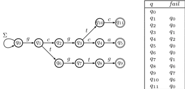
4.2 The Aho-Corasick NFA . . . 46
4.3 The suffix NFA . . . 48
4.4 Bit-parallel simulation of NFAs for the multiple string matching problem . . . 50
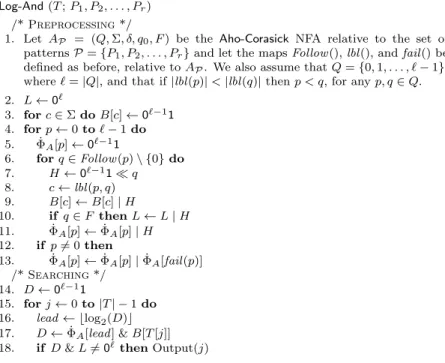
4.5 Bit-parallel simulation of the Aho-Corasick NFA for a set of patterns 51 4.5.1 The Log-And algorithm . . . 53
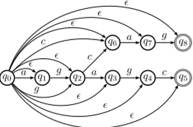
4.6 Bit-parallel simulation of the suffix NFA for a set of patterns . . . 55
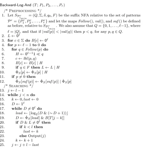
4.6.1 The Backward-Log-And algorithm . . . 59
5 The approximate string matching problem 63 5.1 String matching with swaps . . . 64
5.1.1 Preliminary definitions . . . 65
5.1.2 The Approximate-Cross-Sampling algorithm . . . 67
5.1.3 New algorithms for the approximate swap matching problem 69 5.1.4 Experimental evaluation . . . 76
5.2 Approximate string matching with inversions and translocations . 80 5.2.1 Preliminary definitions . . . 80
5.2.2 An automaton-based approach for the pattern matching problem with translocations and inversions . . . 81
5.2.3 Complexity analysis . . . 88
5.2.4 A bit-parallel implementation . . . 93
5.2.5 Computing the minimum cost . . . 94
5.2.6 Experimental evaluation . . . 96
6 The compressed string matching problem 99 6.1 String matching on Huffman encoded texts . . . 100
6.1.1 Preliminary definitions . . . 102
6.1.2 Skeleton tree based verification . . . 104
6.1.3 Adapting two Boyer-Moore-like algorithms for searching Huffman encoded texts . . . 107
6.1.4 Experimental evaluation . . . 110
6.2 String matching on BWT-encoded texts . . . 113
6.2.2 Searching on BWT-encoded texts . . . 115 6.2.3 A new efficient approach for online searching BWT-encoded
texts . . . 117 6.2.4 Experimental evaluation . . . 122
7 Conclusions 127
Introduction
One of the oldest methods to represent information is by means of written texts. A text can be defined as a coherent sequence of symbols which encodes informa-tion in a specific language. One obvious example are natural languages, which are typically used by humans to communicate in oral or written form. Other exam-ples are DNA, RNA and protein sequences; DNA and RNA are nucleic acids that carry the genetic information of living beings and can be represented as sequences of the nucleobases (Cytosine, Guanine, Adenine and Thymine or Uracil) of their nucleotides. Proteins are molecules made of amino acids that are fundamental constituents of living organisms and can be represented by the sequence of amino acids (20 in total) encoded in the corresponding gene.
A natural problem which arises when dealing with such sequences is identify-ing specific patterns; as far as natural language texts are concerned, one is often interested in finding the occurrences of a given word or sentence; on the other side, an important problem in computational biology is finding given features in DNA sequences or determining the degree of similarity of two sequences. Both problems are particular instances of the string matching problem which has been investigated in a formal way since 1970 [30, 57].
Among other applications of the string matching problem we recall data scan-ning problems, such as intrusion detection or anti-virus scanscan-ning, and searching of patterns within images (which can be modelled as two-dimensional sequences). Formally, given an alphabet of symbols Σ of size σ, a text T of n symbols and a pattern P of m symbols, the string matching problem consists in finding all positions in T in which P occurs. In its online version only the pattern can
be preprocessed before searching; instead, in the offline version the text can be preprocessed to build a suitable data structure that allows searching for arbitrary patterns without traversing the whole text.
In this thesis we deal with online string matching only. The first linear so-lution for the string matching problem is the Knuth-Morris-Pratt algorithm [47], which solves the problem with O(n) worst-case searching time complexity and O(m)-space complexity. This algorithm is based on the deterministic finite au-tomaton for the language Σ∗P and scans the text from left to right. The first
sublinear string matching algorithm is due to Boyer and Moore [14]. The Boyer-Moorealgorithm processes the text in windows of size m and scans each window from right to left. The idea is to stop when a mismatch occurs and then shift the window based on the characters read. The algorithm is quadratic in the worst case though, on the average, it shows a sublinear behaviour. Another important solutiond based on finite automata is the Backward-DAWG-Matching algorithm (BDM) [30], which uses the deterministic automaton for the language Suff (P ) of the suffixes of P (suffix automaton) [11]; in this case the text is processed in windows of size m and windows are scanned from right to left, as the Boyer-Moorealgorithm. When a mismatch occurs, the window is shifted according to the length of the longest recognized prefix of the pattern that is aligned with the right side of the window. The algorithm hasO(mn) worst-case time complexity andO(m)-space complexity.
The optimal average time complexity of the string matching problem, under a Bernoulli model of probability where all the symbols are equiprobable, is equal toO(n logσ(m)/m) [70]. Such a bound has been achieved by the BDM algorithm.
Another important finite automaton for the string matching problem is the factor oracle [2]; this automaton recognizes at least the factors of the input string and can be used in place of the suffix automaton in the BDM algorithm (this variant is known as BOM). The advantage of this automaton is that it is lighter because it has m + 1 states, as opposed to the suffix automaton which can have up to 2m− 1 states. Although the solutions based on finite automata are suitable from a theoretical point of view, in practice they do not always perform well. Indeed, the algorithm which is usually implemented in computer programs is a simplified version of the Boyer-Moore algorithm due to Horspool [39]. The principle of simplicity is very relevant in string matching algorithms.
The situation changed in 1992 when Baeza-Yates and Gonnet introduced the technique known as bit-parallelism to simulate the nondeterministic version of
the Knuth-Morris-Pratt automaton [8]. They devised a new algorithm, named Shift-And, which is a version of the Knuth-Morris-Pratt algorithm based on the nondeterministic finite automaton (NFA) recognizing Σ∗P . The virtue of this
algorithm is that it is extremely simple and succint, thus achieving very good performance in practice. Bit-parallelism is a representation, based on bit-vectors, that exploits the regularity of some nondeterministic automata. The space needed by this encoding isO(σ⌈m/w⌉), where w is the size in bits of a computer word. Later, Navarro and Raffinot extended this result to the nondeterministic version of the suffix automaton [56]. They presented an algorithm, named BNDM, which is the version of the BDM algorithm based on the NFA for the language Suff (P ). Despite being very efficient in practice, algorithms based on bit-parallelism suffer from an intrinsic limitation: they have aO(⌈m/w⌉) overhead in the corresponding time complexity, which is due to the use of a representation based on bit-vectors. Hence, they do not scale efficiently as the pattern length grows. A few techniques have been proposed to workaround this limitation [56, 59], but they all have some drawbacks.
A natural generalization of the string matching problem is the multiple string matching problem: given a setP of patterns and a text T , the multiple string matchingproblem is tantamount to finding all the occurrences in T of the patterns inP. The first linear solution for this problem based on finite automata is due to Aho and Corasick [1]. The Aho-Corasick algorithm uses a deterministic incomplete finite automaton for the language Σ∗P based on the trie for the input patterns,
and is basically a generalization of the Knuth-Morris-Pratt algorithm. The first sublinear solution is due to Commentz-Walter [27] and is a generalization of the Boyer-Moorealgorithm based on the trie for the input patterns. Generalizations of the BDM and of the BOM algorithms can be found in [57]. The nondeterministic versions of finite automata for the multiple string matching problem are more difficult to simulate because, in general, it is not true that for every state the number of outgoing edges is at most 1, which is one of the properties exploited by bit-parallelism. Nevertheless, there exist generalizations of the Shift-And and of the BNDM algorithms [57] that are based on a simplified trie in which no factoring of prefixes occurs.
An important variant of the string matching problem is the approximate string matching problem, which consists in finding all the occurrences of a pattern in a text allowing for a finite number of errors. Errors are formalized by means of a distance function on strings which maps two strings into the minimal cost of
a sequence of edit operations that are needed to convert the first string into the second string. This problem is useful to find, for example, DNA subsequences af-ter mutations, or spelling errors. Well known distance functions for this problem are the edit distance [49] (also called the Levenshtein distance) or the Damerau edit distance [31]. The edit operations in the former edit distance are insertion, deletion, and substitution of characters; instead, in the second case, one allows for swaps of characters, i.e., transpositions of two adjacent characters1. Approximate
string matching under the Damerau distance is also known as string matching with swaps and was introduced in 1995 as one of the open problems in non-standard string matching [52]. A variant of this problem, known as approximate string matching with swaps, consists in computing, for each occurrence, also the corresponding number of swaps.
Another important variant of the string matching problem is the compressed string matchingproblem, which consists in searching for a pattern in a text stored in a compressed form. Compression in this case means reducing the size of the text representation without any loss of information, i.e., the original text can be completely recovered from its compressed version. Despite the fact that the price of external memory has lowered dramatically in recent years, the interest in data compression has not withered; hence, being able to perform text processing directly on the compressed text remains an interesting task. The two compression methods that are investigated in this thesis are prefix codes and the Burrows-Wheeler transform. Prefix codes are variable-length codes with the property that no codeword is a prefix of any other codeword in the set. This compression method is also known as Huffman coding [40]. The problem which arises when performing string matching on prefix codes is that decoding must be performed from left to right and no bit can be skipped. The Burrows-Wheeler transform [15] (BWT) is a reversible transformation which yields a permutation of the text that can be better compressed using the combination of a locally-adaptive encoding, such as move-to-front [10], and statistical methods [40, 67]. It is not possible to search for a pattern in a BWT encoded text without preprocessing the text once at least. Hence, Existing algorithms [9] for string matching on BWT encoded texts are not strictly online. These algorithms are able to compute how many times a given pattern occurs in a text and all the positions in which it occurs, but require more than one iteration over the compressed text.
1.1
Results
The main results presented in this thesis are:
• a new encoding, based on bit-vectors, for regular NFAs as those for the languages Σ∗P and Suff (P ). The new representation, based on a particular
factorization of strings, requires O(σ⌈k/w⌉) space and adds a O(⌈k/w⌉) overhead to the time complexity of the algorithms based on it, where⌈m
σ⌉ ≤
k≤ m is the size of the factorization and m is the length of the input string. We show that bit-parallel string matching algorithms based on this encoding scale much better as m grows.
• a new encoding, based on bit-vectors, of the NFA for the language
P∈PΣ∗P
induced from the trie data structure for P and the NFA for the language
P∈PSuff(P ) induced from the DAWG data structure for P. The new
representation requiresO((σ + m)⌈m/w⌉) space, where m is the number of states of the automaton.
• practical bit-parallel variants of the Wide-Window algorithm that exploit the bit-level parallelism to simulate two automata in parallel. In one case this approach makes it possible to double the shift performed by the algorithm. • the definition of a distance for approximate string matching based on edit operations that involve substrings of the string, namely swaps of equal length adjacent substrings and reversal of substrings; we also present an al-gorithm, based on dynamic programming and on the DAWG data structure, to solve the approximate string matching problem under this distance. • a simple variant of an algorithm for the string matching with swaps problem
that is able to count, for each occurrence of the pattern, the corresponding number of swaps without any time and space overhead.
• a general algorithm designed to adapt Boyer-Moore like algorithms for com-pressed string matchingin Huffman encoded texts; the new algorithm is able to skip bits when decoding.
• a new type of preprocessing for online string matching on BWT encoded texts to count the occurrences of a pattern; the new algorithms require one iteration only over the compressed text and use less space, on average, in the case of moderately large alphabets.
This thesis includes material from my original publications [21, 17, 24, 25, 23, 22, 18].
1.2
Organization of the thesis
The thesis is divided into seven chapters. Chapter 2 provides the reader with the basic notions needed to properly follow the results presented in the subsequent chapters; in particular, it introduces the basic notions and notations used to work with strings and finite state automata and also specifies some basic data structures. Chapter 3 focuses on the basic string matching problem; it presents a formal derivation of the solutions for this problem based on nondeterministic finite automata and on the bit-parallelism technique and includes some novel results as well. Chapter 4 deals with the multiple string matching problem and presents existing and novel results concerning methods based on nondeterministic finite automata and bit-parallelism. Chapters 5 and 6 focus on more complex variants of the string matching problem such as approximate string matching and compressed string matching, respectively, and present novel results for both problems. The conclusions are finally drawn in Chapter 7.
Basic notions and definitions
2.1
Strings
A string P of length |P | = m over a given finite alphabet Σ of size σ is any sequence of m characters of Σ. For m = 0, we obtain the empty string ε. Σ∗
is the collection of all finite strings over Σ. We denote by P [i] the (i + 1)-th character of P , for 0≤ i < m. Likewise, the substring (or factor) of P contained between the (i + 1)-th and the (j + 1)-th characters of P is denoted by P [i .. j], for 0 ≤ i ≤ j < m. We also put Pi =Def P [0 .. i], for 0 ≤ i < m, and make
the convention that P−1 denotes the empty string ε. It is common to identify a string of length 1 with the character occurring in it. We also put first(P ) = P [0] and last(P ) = P [|P | − 1].
For any two strings P and P′, we write P.P′ or, more simply, P P′ to denote
the concatenation of P′ with P . We also write P′ ⊒ P (P′ A P ) to indicate
that P′ is a (proper) suffix of P , i.e., P = P′′.P′ for some nonempty string P′′.
Analogously, P′ ⊑ P (P′ @ P ) denotes that P′ is a (proper) prefix of P , i.e.,
P = P′.P′′ for some (nonempty) string P′′. We denote by Fact(P ) the set of the
factors of P and by Suff (P ) the set of the suffixes of P . We write Pr to denote
the reverse of the string P , i.e., Pr = P [m
− 1]P [m − 2] . . . P [0]. Given a finite set of patternsP, let Pr =
Def{P
r
| P ∈ P} and Pl =Def{P [0 .. l − 1] | P ∈ P}.
We also define size(P) =Def
P∈P|P | and extend the maps Fact(·) and Suff (·)
toP by putting Fact(P) =Def
P∈PFact(P ) and Suff (P) =Def
P∈PSuff(P ).
2.2
Nondeterministic finite automata
A nondeterministic finite automaton (NFA) with ε-transitions is a 5-tuple N = (Q, Σ, δ, q0, F ), where Q is a set of states, q0 ∈ Q is the initial state, F ⊆ Q is
the collection of final states, Σ is an alphabet, and δ : Q× (Σ ∪ {ε}) → P(Q) is the transition function (P(·) is the powerset operator).1 For each state q
∈ Q, the ε-closure of q, denoted as ECLOSE(q), is the set of states that are reachable from q by following zero or more ε-transitions. ECLOSE can be generalized to a set of states by putting ECLOSE(D) =Def
q∈DECLOSE(q). In the case of an
NFA without ε-transitions, we have ECLOSE(q) ={q}, for any q ∈ Q.
The extended transition function δ∗: Q× Σ∗→ P(Q) induced by δ is defined
recursively by δ∗(q, u) =Def ECLOSE(q) if u = ε,
p∈δ∗(q,v)ECLOSE(δ(p, c)) if u = v.c, for some c∈ Σ and v ∈ Σ∗.
In particular, when no ε-transition is present, then
δ∗(q, ε) ={q} and δ∗(q, v.c) = δ(δ∗(q, v), c) .
Both the transition function δ and the extended transition function δ∗can be
naturally generalized to handle set of states, by putting δ(D, c) =Def q∈Dδ(q, c)
and δ∗(D, u) =Def
q∈Dδ∗(q, u), respectively, for D ⊆ Q, c ∈ Σ, and u ∈ Σ∗.
The extended transition function satisfies the following property:
δ∗(q, u.v) = δ∗(δ∗(q, u), v), for all u, v∈ Σ∗. (2.1)
Given an NFA N = (Q, Σ, δ, q0, F ), we define a reachable configuration of N any
subset D⊆ Q such that D = δ∗(q
0, u), for some u∈ Σ∗.
2.3
Bitwise operators on computer words and
the bit-vector data structure
We recall the notation of some bitwise infix operators on computer words, namely the bitwise and “&”, the bitwise or “|”, the left shift “≪” and right shift
1In the case of NFAs with no ε-transitions, the transition function has the form δ : Q × Σ →
“≫” operators (which shifts to the left (right) its first argument by a number of bits equal to its second argument), and the unary bitwise not operator “∼”.
The functions that compute the first and the last bit set to 1 of a word x are ⌊log2(x & (∼ x + 1))⌋ and ⌊log2(x)⌋, respectively. Modern architectures include
assembly instructions for this purpose; for example, the x86 family provides the bsf and bsr instructions, whereas the powerpc architecture provides the cntlzw instruction. For a comprehensive list of machine-independent methods for computing the index of the first and last bit set to 1, see [7].
A setS ⊆ {1, 2, . . . , m} of integers can be conveniently represented as a vector D of m bits. The i-th bit of D is set to 1 if the element i belongs to S, to 0 otherwise. If w is the size in bits of a computer word, ⌈m/w⌉ words are needed to represent S. Using this representation, typical operations on sets map onto simple bitwise operations:
• i ∈ S ⇐⇒ (D & (1 ≪ i)) ̸= 0 • S ∪ {i} ⇐⇒ D | (1 ≪ i) • S1∪ S2 ⇐⇒ D1| D2 • S1∩ S2 ⇐⇒ D1& D2 • S1\ S2 ⇐⇒ D1&∼ D2 • Sc ⇐⇒ ∼ D .
This representation allows to exploit the bit-level parallelism of the operations on computer words, cutting down the number of operations that an algorithm performs by a factor of w, as the time complexity of each operation is Θ(⌈m/w⌉).
2.4
The trie data structure
Given a setP of patterns over a finite alphabet Σ, the trie TP associated withP
is a rooted directed tree, whose edges are labeled by single characters of Σ, such that
(i) distinct edges out of a same node are labeled by distinct characters; (ii) all paths inTP from the root are labeled by prefixes of the strings inP;
(a) q0 q1 q2 q3 q4 q5 q6 q7 q8 q9 q10 q11 g c g c a t g t g t c (b) q0 q1 q2 q3 q4 q5 q6 q7 q8 q9 q10 q13 q14 q15 q16 q17 g c g c a g c g t c g t g t g
Figure 2.1: (a) trie and (b) maximal trie for the set of strings {gcgca,gtgtg,gcgtc}.
(iii) for each string P in P there exists a path in TP from the root which is
labeled by P .
For any node p in the trieTP, we denote by lbl (p) the string which labels the
path from the root of TP to p and put len(p) =Def|lbl(p)|. Plainly, the map lbl
is injective. Additionally, for any edge (p, q) inTP, the label of (p, q) is denoted
by lbl (p, q).
For a set of patterns P = {P1, P2, . . . , Pr} over an alphabet Σ, the maximal
trieofP is the trie Tmax
P obtained by merging into a single node the roots of the
linear triesTP1,TP2, . . . ,TPr relative to the patterns P1, P2, . . . , Pr, respectively.
Strictly speaking, the maximal trie is a nondeterministic trie, as property (i) above may not hold at the root. An example of trie and maximal trie is shown in Fig. 2.1.
2.5
The DAWG data structure
The directed acyclic word graph (DAWG) [11, 28, 30] for a finite set of patternsP is a data structure representing the set Fact(P). To describe it precisely, we need the following definitions. Let us denote by end-pos(u) the set of all positions in P where an occurrence of u ends, for u ∈ Σ∗; more formally, let
end-pos(u) =Def{(P, j) | u ⊒ Pj, with P ∈ P and |u| − 1 ≤ j < |P |} .
For instance, we have end-pos(ε) ={(P, j) | P ∈ P and − 1 ≤ j < |P |}, since ε⊒ Pj, for each P ∈ P and −1 ≤ j < |P | (we recall that P−1= ε, by convention). 2
2In the case of a single pattern, i.e., |P| = 1, end-pos is just a set of positions rather than of
q0 q1 q2 q3 q4 q5 q6 q7 q8 a g c g a c g c a g q suf R q0 {ϵ} q1 q0 {a} q2 q0 {ag, g} q3 q1 {aga, ga} q4 q2 {agag, gag} q5 q6 {agagc, gagc} q6 q0 {agc, gc, c}
q7 q1 {agca, gca, ca}
q8 q2 {agcag, gcag, cag}
Figure 2.2: DAWG for the set of strings {agagc,agcag}.
We also define an equivalence relation RP over Σ∗ by putting
u RP v ⇐⇒Def end-pos(u) = end-pos(v) , (2.2)
for u, v ∈ Σ∗, and denote by R
P(u) the equivalence class of RP containing the
string u. Futhermore, let
val(RP(u)) =Defthe longest string in the equivalence class RP(u) , (2.3)
and length(RP(u)) =Def |val(RP(u))|. Then the DAWG for a finite set P of
patterns is a directed acyclic graph (V, E) with an edge labeling function lbl (), where V = {RP(u)| u ∈ Fact(P)}, E = {(RP(u), RP(uc)) | u ∈ Σ∗, c∈ Σ, uc ∈
Fact(P)}, and lbl(RP(u), RP(uc)) = c, for u∈ Σ∗, c∈ Σ such that uc ∈ Fact(P)
(cf. [12]).
We also define a failure function, suf : Fact(P) \ {ε} → Fact(P), named suffix link, by putting
suf(u) =Def the longest v∈ Suff (u) such that y ̸RPx (2.4)
for u∈ Fact(P) \ {ε}.
The suf (·) and end-pos(·) functions can be extended to the equivalence classes of RP not containing ε, by putting for all q∈ V \ {RP(ε)}
suf(q) =Def RP(suf (val (q)))
end-pos(q) =Def end-pos(val (q)) .
An example of DAWG is shown in Fig. 2.2. The DAWG for a finite set of pat-ternsP naturally induces the deterministic automaton F (P) = (Q, Σ, δ, root, F ) whose language is Fact(P), where
• Q = {RP(u) : u∈ Fact(P)} is the set of states,
• Σ is the alphabet of the characters in P ,
• δ : Q × Σ → Q is the transition function defined by: δ(RP(u), c) = {RP(uc)} if uc ∈ Fact(P) ∅ otherwise
• root = RP(ε) is the initial state,
• F = Q is the set of final states.
2.6
Experimental framework
The experimental results presented in this thesis have been obtained using the following setup: all the algorithms have been implemented in the C program-ming language and have been compiled with the GNU C Compiler 4.0, using the optimization options -O2 -fno-guess-branch-probability; the running times have been measured with a high resolution timer by first copying the whole input in memory and then taking the mean over a certain number of runs of the time needed by the algorithm to end. The word size is 32 in all the tests. The corpus used to carry out the tests consists of the following files:
(i) the English King James version of the “Bible” (n = 4, 047, 392, σ = 63), (ii) the CIA World Fact Book (n = 2, 473, 400, σ = 94),
(iii) a DNA sequence of the Escherichia coli genome (n = 4, 638, 690, σ = 4),
(iv) a protein sequence of the Saccharomyces cerevisiae genome (n = 2, 900, 352, σ = 20),
(v) the Spanish novel “Don Quixote” by Cervantes (n = 2347740, σ = 86).
where n denotes the number of characters and σ denotes the alphabet size. Files (i), (ii), and (iii) are from the Canterbury Corpus 3, file (iv) is from the Protein
Corpus4, and file (v) is from Project Gutenberg5.
3
http://corpus.canterbury.ac.nz/
4http://data-compression.info/Corpora/ProteinCorpus/ 5http://www.gutenberg.org/
The string matching
problem
Given a pattern P of length m and a text T of length n, both drawn from a common finite alphabet Σ of size σ, the string matching problem consists in finding all the occurrences of P in T . The optimal average time complexity of the problem is equal toO(n logσ(m)/m) [70].
The most efficient solutions for the string matching problem are based on finite automata. As already recalled, the first linear-time solution is the Knuth-Morris-Pratt algorithm [47]. This algorithm uses an implicit representation of the automaton for the language Σ∗P based on the border function of the
pat-tern [30] and solves the problem withO(n) worst-case searching time complexity andO(m)-space complexity. The lower bound on average has been achieved by the BDM algorithm [30], that is based on the deterministic automaton for the language Suff (P ). The worst-case searching time complexity of this algorithm is O(mn) while its space complexity is O(m). Baeza-Yates and Gonnet [8] in-troduced a technique, known as bit-parallelism, to simulate the nondeterministic versions of these automata. They devised a new algorithm, named Shift-And, that is the version of the Knuth-Morris-Pratt algorithm based on the NFA recognizing Σ∗P . Later, Navarro and Raffinot [56] presented the BNDM algorithm, which is
the version of the BDM algorithm based on the nondeterministic suffix automa-ton for the language Suff (P ). Albeit algorithms based on bit-parallelism are very efficient and compact, they have an O(⌈m/w⌉) overhead, where w is the size in
bits of a computer word, as compared to the corresponding algorithms based on a deterministic automaton. This limitation is intrinsic, since the bit-parallelism encoding is based on bit-vectors.
In this chapter we present new results concerning bit-parallelism. In tion 3.1 we formally define the NFAs for the string matching problem and in Sec-tion 3.2 we introduce the bit-parallelism technique and the two main algorithms based on it. Then, in Section 3.3 we present a new encoding, based on bit-vectors, for regular NFAs as those for the languages Σ∗P and Suff (P ). By exploiting a
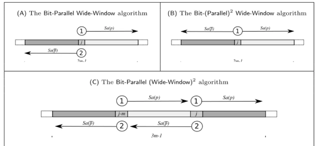
particular factorization of strings, the new representation allows to encode au-tomata by smaller bit-vectors resulting in faster algorithms. In Section 3.4 we present a method to increase the parallelism in bit-parallel algorithms; more pre-cisely, we introduce variants of the Wide-Window algorithm [37] that simulate two automata in parallel. In one case this approach makes it possible to double the shift performed by the algorithm at each iteration.
3.1
Automata based solutions for the string
match-ing problem
There are two main automata which are the core building blocks in different algorithms for the string matching problem. Let P ∈ Σmbe a string of length m.
The first automaton is the one for the language Σ∗P , i.e., the automaton that recognizes all the strings that have P as suffix. The second one is the so called suffix automaton, which is the automaton that recognizes the language Suff (P ) of the suffixes of P . It is important to observe that the nondeterministic versions of these automata are very regular. We indicate withA (P ) = (Q, Σ, δ, q0, F ) the
nondeterministic automaton for the language Σ∗P , where:
• Q = {q0, q1, . . . , qm} (q0 is the initial state)
• the transition function δ : Q × Σ −→ P(Q) is defined by:
δ(qi, c) =Def {q0, q1} if i = 0 and c = P [0] {q0} if i = 0 and c̸= P [0]
{qi+1} if 1≤ i < m and c = P [i]
(a) 0 1 2 3 4 Σ a t a g (b) I 0 a 1 t 2 a 3 g 4 ǫ ǫ ǫ ǫ ǫ
Figure 3.1: (a) Nondeterministic automaton and (b) nondeterministic suffix automa-ton for the pattern atag.
• F = {qm} (F is the set of final states).
Likewise, we denote by S (P ) = (Q, Σ, δ, I, F ) the nondeterministic suffix automaton with ε-transitions for the language Suff (P ), where:
• Q = {I, q0, q1, . . . , qm} (I is the initial state)
• the transition function δ : Q × (Σ ∪ {ε}) −→ P(Q) is defined by:
δ(q, c) =Def
{qi+1} if q = qi and c = P [i] (0≤ i < m)
Q if q = I and c = ε
∅ otherwise
• F = {qm} (F is the set of final states).
An example of both automata is shown in Fig. 3.1.
The algorithms based on the automataA (P ) and S (P ) for searching a pat-tern P in a text T work by moving a logical window of size |P | over T . The method based on the automatonA (P ) computes, for a given window ending at position j in T , all the prefixes of P that are suffixes of Tj. In particular, there
is an occurrence of P if the prefix of length m is found. The algorithm always shifts the current window by one position to the right, i.e., it checks every win-dow. Instead, the method based on the automatonS (P ) computes, for a given window ending at position j in T , the longest prefix of P that is a suffix of Tjby
reading the window from right to left with S (Pr). As in the previous method, there is an occurrence of P if the length of the longest prefix found is m. The algorithm shifts the current window by a number of positions that depends on the length of the longest proper prefix of P recognized. This approach makes it possible to skip windows.
Given a pattern P of length m, the automaton A (P ) can be used to find the occurrences of P in a given text T , by observing that P has an occurrence in T ending at position i, i.e., P ⊒ Ti, if and only if δ∗A(q0, T [0 .. i]) contains the final
state qm. Thus, to find all the occurrences of P in T , it suffices to compute the
set δ∗
A(q0, Ti)∩ F , for i = 0, 1, . . . , |T | − 1.
Given a pattern P of length m, the automatonS (Pr) can be used to find the
occurrences of P in a text T by observing that P has an occurrence in T ending at position i, i.e., P ⊒ Ti, if and only if δS∗r(q0, (T [i− m + 1 .. i])r) contains the
final state qm. Hence, to find all the occurrences of P in T , one can compute
δ∗
Sr(q0, (T [i− m + 1 .. i])r)∩ F , for i = m − 1, m, . . . , |T | − 1. With this approach
it is possible to skip windows: in fact, for a window of T of size m ending at position i, let l be the length of the longest proper suffix of T [i− m + 1 .. i] such that δS∗r(q0, (T [i− l + 1 .. i])r)∩ F ̸= ∅. It is easy to see that l is the length of
the longest prefix of P that is a suffix of Ti. Then, the windows at positions
i, i + 1, . . . i + m− l − 1 can be safely skipped.
3.2
The bit-parallelism technique
Bit-parallelism is a technique, based on bit-vectors, that was introduced by Baeza-Yates and Gonnet in [8] to simulate efficiently nondeterministic automata. The first algorithms based on this technique are the well-known Shift-And [8] and BNDM[56]. The trivial way to encode a nondeterministic automaton of m states is by i) finding a linear ordering of its states, ii) representing the automaton configurations as bit vectors, such that bit i is set iff state with position i is active, and iii) by tabulating the transition function δ(D, c), for D ⊆ Q, c ∈ Σ. However, the main problem of this representation is that the space in bits needed to represent the transition function is (2m
· σ) · m, which is exponential in m. Bit-parallelism takes advantage of the regularity of the automataA (P ) and S (P ) to efficiently encode the transition function in a different way. The construction can be derived by starting from a result that was first formalized for the Glushkov automaton and that can be immediately generalized to a certain class of NFAs as follows (cf. [58]).
Let N = (Q, Σ, δ, q0, F ) be an NFA with ε-transitions such that up to the
ε-transitions, for each state q∈ Q, either
B=
σ q1 q2 q3 q4
a 1 0 1 0 t 0 1 0 0 g 0 0 0 1
Figure 3.2: The map B(·) of the automatonA (atag).
(ii) all the incoming transitions in q originate from a unique state.
Let B(c), for c∈ Σ, be the set of states of N with an incoming transition labeled by c, i.e.,
B(c) =Def{q ∈ Q | q ∈ δ(p, c), for some p ∈ Q} .
Likewise, let Follow (q), for q∈ Q, be the set of states reachable from state q with one transition over a character in Σ, i.e.,
Follow(q) =Def c∈Σ δ(q, c) . and let Φ(D) =Def q∈D Follow(q) ,
for D⊆ Q. Then the following result holds.
Lemma 3.1 (cf. [58]). For every q∈ Q, D ⊆ Q, and c ∈ Σ, we have (a) δ(q, c) = F ollow(q)∩ B(c);
(b) δ(D, c) = Φ(D)∩ B(c).
Proof. Concerning (a), we notice that δ(q, c)⊆ F ollow(q)∩B(c) holds plainly. To prove the converse inclusion, let p∈ F ollow(q) ∩ B(c). Then p ∈ δ(q, c′)∩ δ(q′, c),
for some c′ ∈ Σ and q′∈ Q. If p satisfies condition (i), then c′= c, and therefore
p ∈ δ(q, c). On the other hand, if p satisfies condition (ii), then q = q′ and
therefore p∈ δ(q, c) follows again.
From (a), we obtain immediately (b), since δ(D, c) = q∈D δ(q, c) = q∈D (Follow (q)∩ B(c)) = q∈D Follow(q)∩ B(c) = Φ(D) ∩ B(c) .
Shift-And(P , m, T , n) 1. for c∈ Σ do B[c] ← 0m 2. for i← 0 to m − 1 do 3. B[P [i]] = B[P [i]]| (0m−11 ≪ i) 4. D← 0m 5. for j← 0 to n − 1 do 6. D← ((D ≪ 1) | 0m−11) & B[T [j]] 7. ifD & 10m−1 ̸= 0mthenOutput(j)
Figure 3.3: The Shift-And algorithm.
Provided that one finds an efficient way of storing and accessing the maps Φ(·) and B(·), equation (b) of Lemma 3.1 is particularly suitable for a representation based on bit-vectors, as set intersection can be readily implemented by the bitwise andoperation.
The map B(·) can be encoded with σ ·m bits, independently of the automaton structure, using an array B of σ bit-vectors, each of size m, where the i-th bit of B[c] is set if there is an incoming transition in state with position i labeled by c. Instead, a generic encoding of the Φ(·) map requires 2m· m bits, which is
exponential in the number m of states.
While this result allows to reduce the total bits needed to represent the tran-sition function to (2m+ σ)· m, it can still be improved. In fact, depending on
the automaton structure, it is possible to find a more efficient way to compute the map Φ(·).
3.2.1
The Shift-And algorithm
The Shift-And algorithm simulates the nondeterministic automaton that recog-nizes the language Σ∗P , for a given string P of length m. An Automaton
con-figuration δ∗(q
0, S) on input S∈ Σ∗ is encoded as a bit-vector D of m bits (the
initial state does not need to be represented as it is always active), where the i-th bit of D is set to 1 iff state qi+1is active, i.e., qi+1∈ δ∗(q0, S), for i = 0, . . . , m−1.
The map B(·) is encoded, as described above, using an array B of σ bit-vectors, each of size m, where the i-th bit of B[c] is set iff δ(qi, c) = qi+1 or equivalently
iff P [i] = c, for c ∈ Σ, 0 ≤ i < m. An example of the B(·) map is shown in Fig. 3.2. As far as the Φ(·) map is concerned, observe that Follow(qi) ={qi+1},
config-uration D,
Φ(D) =
qi∈D
{qi+1} ∪ {q0} ,
which becomes
qi∈D{qi+1}∪{q1} if we do not represent the initial state. Hence,
if D is represented as a bit-vector, we can compute Φ(D) with a bitwise left shiftoperation of one unit and a bitwise or with 1 (represented as 0m−11).
For a configuration D of the NFA, a transition on character c can then be implemented by the bitwise operations
D← ((D ≪ 1) | 1) & B[c] .
When a search starts, the initial configuration D is initialized to 0m. Then,
the automaton configuration is updated for each text character, as described before, by reading the text from left to right. For each position j in T , if D is the automaton configuration after having read the j-th character, it holds that Pi ⊒ Tj iff bit i is set in D. Thus, to verify if there is a match at position j it
suffices to check that the (m−1)-th bit is set in D. The worst-case searching time complexity of the Shift-And algorithm isO(n⌈m/w⌉) while the space complexity isO(σ⌈m/w⌉). The pseudocode of the algorithm is shown in Fig. 3.3.
3.2.2
The Backward-Nondeterministic-DAWG-Matching
algo-rithm
The Backward-Nondeterministic-DAWG-Matching algorithm (BNDM, for short) sim-ulates the nondeterministic suffix automaton for Prwith the bit-parallelism
tech-nique, using an encoding similar to that described above for the Shift-And algo-rithm. The automaton configuration is encoded again as a bit vector D of m bits. The i-th bit of D is set to 1 iff state qi+1 is active, for i = 0, 1, . . . , m− 1,
and D is initialized to 1m, since after the ε-closure of the initial state I all states
qirepresented in D are active. The first transition on character c is implemented
as D ← (D & B[c]), while any subsequent transition on character c can be implemented as
D← ((D ≪ 1) & B[c]) .
This algorithm works by shifting a window of length m over the text. Specifi-cally, for each window alignment, it searches the pattern by scanning the current window backwards and updating the automaton configuration accordingly.
BNDM(P , m, T , n) 1. for c∈ Σ do B[c] ← 0m 2. for i← 0 to m − 1 do 3. c← P [m − 1 − i] 4. B[c] = B[c]| (0m−11≪ i) 5. j← m − 1 6. while j < n do 7. k← 0, last ← 0 8. D← 1m 9. whileD̸= 0mdo 10. D← D & B[T [j − k]] 11. k← k + 1 12. if D & 10m−1̸= 0mthen 13. ifk > 0 then 14. last← k 15. elseOutput(j) 16. D← D ≪ 1 17. j← j + m − last
Figure 3.4: The Backward-Nondeterministic-DAWG Matching algorithm.
Let j be the ending position of the current window. At each iteration k, for k = 1, . . . , m, the automaton configuration is updated by performing a transition on character T [j− k + 1], as described before. After having performed the k-th transition, it holds that
T [j− k + 1, . . . , j] = P [m − 1 − i, . . . , m − 2 − i + k] iff bit i is set in D, for i = k− 1, . . . , m − 1.
Each time a suffix of Pr (i.e., a prefix of P ) is found, i.e., when prior to the
left shift the (m− 1)-th bit of D & B[c] is set, the suffix length k is recorded in a variable last. A search ends when either D becomes zero (i.e., when no factor of P can be recognized) or when the algorithm has performed m iterations (i.e., when a match has been found). The window is then shifted to the starting position of the longest recognized proper prefix, i.e., to position j + m−last. The worst-case searching time complexity of the BNDM algorithm is O(nm⌈m/w⌉), while its space complexity is O(σ⌈m/w⌉). The algorithm BNDM is optimal on average as BDM. The pseudocode of the algorithm is shown in Fig. 3.4.
3.2.3
Bit-parallelism limitations
When the pattern size m is larger than w, the configuration bit-vector and all auxiliary bit-vectors need to be splitted over ⌈m/w⌉ multiple words. For this
reason the performance of the Shift-And and BNDM algorithms, and, more in general, of bit-parallel algorithms degrade considerably as⌈m/w⌉ grows. A com-mon approach to overcome this problem consists in constructing an automaton for a substring of the pattern fitting in a single computer word, to filter possible candidate occurrences of the pattern. When an occurrence of the selected sub-string is found, a subsequent naive verification phase allows to establish whether it belongs to an occurrence of the whole pattern. However, besides the costs of the additional verification phase, a drawback of this approach is that, in the case of the BNDM algorithm, the maximum possible shift length cannot exceed w, which may be much smaller than m.
3.3
Tighter packing for bit-parallelism
We present a new encoding of the configurations of the nondeterministic (suffix) automaton for a given pattern P of length m, which on the average requires less than m bits and can be used within the bit-parallel framework. The effect is that bit-parallel string matching algorithms based on this encoding scale much better as m grows, at the price of a larger space complexity. We will illustrate such a point experimentally with the Shift-And and the BNDM algorithms, but our proposed encoding can also be applied to other variants of the BNDM algorithm. Our encoding will have the form (D, a), where D is a k-bit vector, with k 6 m (on the average k is much smaller than m), and a is an alphabet symbol (the last text character read) that will be used as a parameter in the bit-parallel simulation with the vector D.
The encoding (D, a) is obtained by suitably factorizing the simple bit-vector encoding for NFA configurations presented in the previous section. More specifi-cally, it is based on the following pattern factorization:
Definition 3.1 (1-factorization). Let P ∈ Σm. A 1-factorization u of size k of
P is a sequence ⟨u1, u2, . . . , uk⟩ of nonempty substrings of P such that:
(a) P = u1u2. . . uk;
(b) each factoruj in u contains at most one occurrence of any of the characters
in the alphabetΣ, for j = 1, . . . , k .
For a given 1-factorization u =⟨u1, u2, . . . , uk⟩ of P , we put
ru
for j = 1, 2, . . . , k + 1 (so that ru
1 = 0 and rk+1u = m) and call the numbers
ru
1, ru2, . . . , ruk+1 the indices of u. Plainly, ruj is the index inP of the first
char-acter of the factor uj, forj = 1, 2, . . . , k.
A 1-factorization of P is minimal if such is its size.
Observe that the size k of a 1-factorization u of a string P ∈ Σmsatisfies the
condition
m σ
≤ k ≤ m .
Indeed, as the length of any factor in u is limited by the size σ of the alphabet Σ, then m ≤ kσ, which implies m
σ ≤ k. The second inequality is immediate
and occurs when P has the form am, for some a
∈ Σ, in which case P has only the 1-factorization of size m whose factors are all equal to the single character string a.
As we shall show below, the size of the bit-vector D in our encoding depends on the size of the 1-factorization used; as a result, a minimal 1-factorization yields the smallest vector. A greedy approach to construct a 1-factorization of smallest size for a string P consists in computing the longest prefix u1of P containing no
repeated characters and then recursively 1-factorize the string P deprived of its prefix u1, as in the procedure Greedy-1-Factorize shown below.
Greedy-1-Factorize(P )
ifP is the empty string ε then returnthe empty sequence⟨ ⟩ else
u1← longest prefix of P containing no repeated character
P′
← the suffix of P such that P = u1P′
returnthe sequence obtained by prepending the factor u1to the
sequence Greedy-1-Factorize(P′)
endif
The correctness of the procedure Greedy-1-Factorize is shown in the following lemma:
Lemma 3.1. The call Greedy-1-Factorize(P ), for a string P ∈ Σm, computes a
minimal 1-factorization of P .
Proof. Let u = ⟨u1, u2, . . . , uk⟩ be the 1-factorization computed by the call
Greedy-1-Factorize(P ) and let v = ⟨v1, v2, . . . , vh⟩ be any 1-factorization of P .
By construction, the character first(ui+1) occurs in ui, for i = 1, 2, . . . , k− 1,
otherwise the factor ui could have been extended by at least one more character.
We say that the factor vjof v covers the factor uiof u if rjv≤ riu< rj+1v (see
(3.1)), i.e., if j is the largest index such that the string v1v2. . . vj−1 is a prefix of
the string u1u2. . . ui−1.
Plainly, each factor of u is covered by exactly one factor of v. Thus, for our purposes, it is enough to show that each factor of v can cover at most one factor of u, so that the number of factors in v must be at least as large as the number of factors in u. Indeed, if this were not the case then
rv
j ≤ rui < rui+1< rj+1v ,
for some i∈ {1, 2, . . . , h} and j ∈ {1, 2, . . . , k}. But then, the string ui.first(ui+1),
which contains two occurrences of the character first(ui+1), would be a factor of
vj, which yields a contradiction.
A 1-factorization⟨u1, u2, . . . , uk⟩ of a given pattern P ∈ Σ∗induces naturally
a partition{Q1, . . . , Qk} of the set Q \ {q0} of states of the automaton A (P ) =
(Q, Σ, δ, q0, F ) for the language Σ∗P , where
Qi =Defqri+1, . . . , qri+1 , for i = 1, . . . , k ,
and r1, r2, . . . , rk+1are the indices of⟨u1, u2, . . . , uk⟩.
Notice that the labels of the arrows entering the states qri+1, . . . , qri+1,
in that order, form exactly the factor ui, for i = 1, . . . , k. Hence, if for any
alphabet symbol a we denote by Qi,a the collection of states in Qi with an
incoming arrow labeled a, it follows that |Qi,a| ≤ 1 since, by condition (b) of
the above definition of 1-factorization, no two states in Qican have an incoming
transition labeled by the same character. When Qi,a is nonempty, we write qi,a
to indicate the unique state q of A (P ) for which q ∈ Qi,a, otherwise qi,a is
undefined. Upon using qi,a in any expression, we also implicitly assert that qi,a
is defined.
For any valid configuration δ∗(q0, Sa) of the automatonA (P ) on some input
of the form Sa∈ Σ∗, we have that q ∈ δ∗(q
in-coming transition labeled a. Therefore, Qi∩ δ∗(q0, Sa)⊆ Qi,aand, consequently,
|Qi∩ δ∗(q0, Sa)| ≤ 1, for each i = 1, . . . , k. The configuration δ∗(q0, Sa) can then
be encoded by the pair (D, a), where D is the bit-vector of size k such that D[i] is set iff Qi contains an active state, i.e., Qi∩ δ∗(q0, Sa)̸= ∅, iff qi,a∈ δ∗(q0, Sa).
Indeed, if i1, i2, . . . , il are all the indices i for which D[i] is set, we have that
δ∗(q
0, Sa) = {qi1,a, qi2,a, . . . , qil,a} holds, which shows that the above encoding
(D, a) can be inverted.
To illustrate how to compute D′in a transition (D, a)−→ (DA ′, c) on character
c using bit-parallelism, it is convenient to give some further definitions.
For i = 1, . . . , k− 1, we put ui= ui.first(ui+1). We also put uk = uk and call
each set ui the closure of ui.
Plainly, any 2-gram can occur at most once in the closure ui of any factor of
our 1-factorization⟨u1, u2, . . . , uk⟩ of P . We can then encode the 2-grams present
in the closure of the factors ui by a σ× σ matrix B of k-bit vectors, where the
i-th bit of B[c1][c2] is set iff the 2-gram c1c2 is present in ui or, equivalently, iff
(last(ui)̸= c1∧ qi,c2 ∈ δ(qi,c1, c2))∨
(i < k∧ last(ui) = c1∧ qi+1,c2 ∈ δ(qi,c1, c2)) ,
(3.2)
for every 2-gram c1c2∈ Σ2and i = 1, . . . , k.
To properly take care of transitions from the last state in Qito the first state
in Qi+1, it is also useful to have an array L, of size σ, of k-bit vectors encoding,
for each character c∈ Σ, the collection of factors ending with c. More precisely, the i-th bit of L[c] is set iff last(ui) = c, for i = 1, . . . , k.
We show next that the matrix B and the array L, which in total require (σ2+ σ)k bits, are all is needed to compute the transition (D, a) A
−→ (D′, c) on
character c. To this purpose, we first state the following basic property, which can easily be proved by induction.
Lemma 3.2 (Transition Lemma). Let (D, a) −→ (DA ′, c), where (D, a) is the
encoding of the configurationδ∗(q
0, Sa) for some string S∈ Σ∗, so that(D′, c) is
the encoding of the configurationδ∗(q0, Sac).
Then, for each i = 1, . . . , k, qi,c∈ δ∗(q0, Sac) if and only if either
(i) last(ui)̸= a, qi,a∈ δ∗(q0, Sa), and qi,c∈ δ(qi,a, c), or
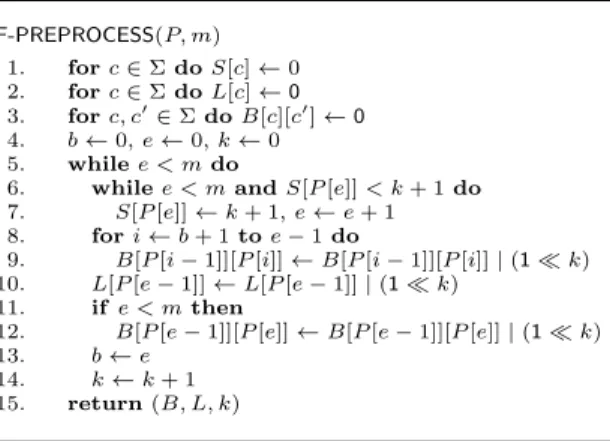
F-PREPROCESS(P, m) 1. forc∈ Σ do S[c] ← 0 2. forc∈ Σ do L[c] ← 0 3. forc, c′ ∈ Σ do B[c][c′] ← 0 4. b← 0, e ← 0, k ← 0 5. whilee < m do
6. whilee < m and S[P [e]] < k + 1 do 7. S[P [e]]← k + 1, e ← e + 1 8. fori← b + 1 to e − 1 do 9. B[P [i− 1]][P [i]] ← B[P [i − 1]][P [i]] | (1 ≪ k) 10. L[P [e− 1]] ← L[P [e − 1]] | (1 ≪ k) 11. if e < m then 12. B[P [e− 1]][P [e]] ← B[P [e − 1]][P [e]] | (1 ≪ k) 13. b← e 14. k← k + 1 15. return(B, L, k)
Figure 3.5: Preprocessing procedure for the construction of the arrays B and L relative to a minimal 1-factorization of the pattern.
Now observe that, by definition, the i-th bit of D′ is set iff q
i,c ∈ δ∗(q0, Sac)
or, equivalently by the Transition Lemma and (3.2), iff (for i = 1, . . . , k) (D[i] = 1∧ B[a][c][i] = 1 ∧ ∼ L[a][i] = 1)∨
(i≥ 1 ∧ D[i − 1] = 1 ∧ B[a][c][i − 1] = 1 ∧ L[a][i − 1] = 1) iff ((D & B[a][c] &∼ L[a])[i] = 1 ∨ (i ≥ 1 ∧ (D & B[a][c] & L[a])[i − 1] = 1)) iff ((D & B[a][c] &∼ L[a])[i] = 1 ∨ ((D & B[a][c] & L[a]) ≪ 1)[i] = 1) iff ((D & B[a][c] &∼ L[a]) | ((D & B[a][c] & L[a]) ≪ 1))[i] = 1 .
Hence D′ = (D & B[a][c] &∼ L[a]) | ((D & B[a][c] & L[a]) ≪ 1) , so that D′ can
be computed by the following bitwise operations: D ← D & B[a][c] H ← D & L[a]
D ← (D & ∼ H) | (H ≪ 1) .
To check whether the final state qm belongs to a configuration encoded as
(D, a), we have only to verify that qk,a = qm. This test can be broken into two
steps: first, one checks if any of the states in Qkis active, i.e., D[k] = 1; then, one
The whole test can then be implemented with the bitwise test D & 10k−1 & L[a]̸= 0k.
The same considerations also hold for the suffix automaton S (P ). The only difference is in the handling of the initial state. In the case of the automaton A (P ), state q0is always active, so we have to activate state q1when the current
text symbol is equal to P [0]. To do so it is enough to perform a bitwise or of D with 0k−11 when a = P [0], as q
1 ∈ Q1. Instead, in the case of the suffix
automaton S (P ), as the initial state has an ε-transition to each state, all the bits in D must be set, as in the BNDM algorithm.
A drawback of the new encoding is that the handling of the self-loop and of the acceptance condition is more complex with respect to the original encoding. However, it is possible to simplify them at the expense of an overhead of at most two bits in the representation, by forcing the first and last factor in a 1-factorization to have length 1. Note that the handling of the self-loop is relevant for the automatonA (P ) only, while the acceptance condition concerns both the A (P ) and S (P ) automata. In particular, to simplify the handling of the self-loop, we compute a factorization where the length of the first factor is equal to 1. Let⟨v1, v2, . . . , vl⟩ be a minimal 1-factorization of P [1 .. m − 1]; we define the
following 1-factorization⟨u1, u2, . . . , ul+1⟩ of P , where
ui= P [0] if i = 1 vi−1 if 2≤ i ≤ l + 1.
Observe that the size of Q1in the corresponding partition is 1; it follows that to
handle the self-loop one does not need to perform the check a = P [0] but just perform a bitwise or with 0k−11, as there is one state only in the first subset and thus q1,ais undefined for all a̸= P [0].
In a similar way, in order to simplify the acceptance condition, we compute a factorization where the length of the last factor is equal to 1; let⟨v1, v2, . . . , vl⟩ be
a minimal 1-factorization of P [0 .. m− 2]; we define the following 1-factorization ⟨u′ 1, u′2, . . . , u′l+1⟩ of P where u′i= vi if 1≤ i ≤ l P [m− 1] if i = l + 1.
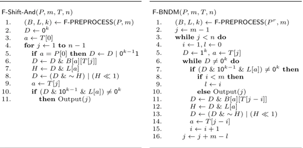
F-Shift-And(P, m, T, n) 1. (B, L, k)← F-PREPROCESS(P, m) 2. D← 0k 3. a← T [0] 4. forj← 1 to n − 1 5. if a = P [0] then D← D | 0k−11 6. D← D & B[a][T [j]] 7. H← D & L[a] 8. D← (D & ∼ H) | (H ≪ 1) 9. a← T [j]
10. if (D & 10k−1& L[a])̸= 0k
11. thenOutput(j) F-BNDM(P, m, T, n) 1. (B, L, k)← F-PREPROCESS(Pr, m) 2. j← m − 1 3. whilej < n do 4. i← 1, l ← 0 5. D← 1k, a ← T [j] 6. whileD̸= 0kdo
7. if(D & 10k−1& L[a])̸= 0kthen
8. ifi < m then 9. l← i 10. elseOutput(j) 11. D← D & B[a][T [j − i]] 12. H← D & L[a]
13. D← (D & ∼ H) | (H ≪ 1) 14. a← T [j − i]
15. i← i + 1 16. j← j + m − l
Figure 3.6: Variants of Shift-And (left) and BNDM (right) based on the 1-factorization encoding.
In this case, the bitwise and with L[a] in the acceptance condition test is not needed anymore, as there is only one state in the last subset.
Let k be the size of a minimal 1-factorization of P . Plainly, in both cases, k− 1 ≤ l ≤ k; in particular, if l = k, we have an overhead of 1 bit. If we combine the two techniques, the overhead in the representation is of at most two bits.
The preprocessing procedure which builds the arrays B and L described above and relative to a minimal 1-factorization of the given pattern P ∈ Σmis reported
in Fig. 3.5. Its time complexity is O(σ2 + m). The variants of the Shift-And
and BNDM algorithms based on our encoding of the configurations of the au-tomata A (P ) and S (P ) are reported in Fig. 3.6 (algorithms F-Shift-And and F-BNDM, respectively). Their worst-case time complexities are O(n⌈k/w⌉) and O(nm⌈k/w⌉), respectively, while their space complexity is O(σ2
⌈k/w⌉), where k is the size of a minimal 1-factorization of the pattern.
3.3.1
q-grams based 1-factorization
It is possible to a achieve higher compactness by transforming the pattern into a sequence of overlapping q-grams and computing the 1-factorization of the result-ing strresult-ing. This technique has been extensively used to boost the performance of several string matching algorithms [36, 60]. More precisely, given a pattern P of length m defined over an alphabet Σ of size σ, the q-gram encoding of P is the
string P0(q)P (q) 1 . . . P
(q)
m−q, defined over the alphabet Σq of the q-grams of Σ, where
Pi(q)= P [i]P [i + 1] . . . P [i + q− 1] ,
i.e., the pattern is transformed into the sequence of its m− q + 1 overlapping substrings of length q, where each substring Pi(q) is regarded as a symbol
be-longing to Σq. Clearly, the size of the 1-factorization of the resulting string is
at least m−q+1
σq . Hence, the size of the 1-factorization can be significantly
re-duced by using a q-grams representation. The only drawback is that the space needed for the tables B and L can grow up to (σ2q + σq)k, where k is the size
of the 1-factorization, if one follows a naive approach. Observe that, for each pairPi(q), Pi+1(q), with i = 0, . . . , m− q − 1, the corresponding transition must be encoded into the table B. However, as we are using overlapping q-grams, we have that Pi(q)[1 .. q− 1] @ P
(q)
i+1, i.e., the last q− 1 symbols of P (q)
i are equal to
the first q− 1 symbols of Pi+1(q). Thus, there is no need to use the full q-gram Pi+1(q) as index in the table, rather we can use only its last symbol. More precisely,
let⟨uq1, u q 2, . . . , u
q
k⟩ be a 1-factorization of the q-gram encoding of P ; we encode
the substrings of length 2q (or, equivalently, the 2-grams over Σq) present in the closure of the factors uqi by a Σq
× Σ matrix B of k bit vectors, where the i-th bit of B[C1][c2] is set iff the substring C1.C1[1 .. q− 1].c2 is present in uqi, for every
C1∈ Σq, c2∈ Σ. This method reduces the space complexity to (σq+1+ σq)k. In
general, however, it is not feasible to use a direct access table for the tables B and T with this encoding.
For values of σq still suitable for a direct access table, a useful technique is
to lazily allocate only the rows of B that have at least one nonzero element. Let gq(P ) be the number of distinct q-grams in P ; then gq(P )≤ min(σq, m− q + 1).
We can have at most gq(P )− 1 nonzero rows in B (there is no transition starting
from the last q-gram), which can be significantly less than σq. The resulting
space complexity is thenO(σq+ (g
q(P )σ + σq)k).
An approach suitable to store the tables B and T , for arbitrary values of q, is to use a hash table, where the keys are the q-grams of the pattern. The main problem which arises when engineering a hash table is to choose a good hash function. Moreover, as we require that lookup in the searching phase be as fast as possible, the hash function must also be very efficient to compute. Since we are using overlapping q-grams, a given q-gram shares q− 1 symbols with the previous one. To exploit this redundancy, we need a hash function that allows a
recursive computation of the hash value of a generic q-gram Xb starting from the hash value of the previous q-gram aX, for|X| ∈ Σq−1 and a, b∈ Σ. A method
that satisfies such a requirement is hashing by integer division, which has been used in the Karp-Rabin string matching algorithm [42]. In this case, the hash function has the following definition
h(s0, s1, . . . , sq−1) = q−1
j=0
rq−j−1ord(sj) mod n , (3.3)
where the radix r and n are parameters and ord : Σ→ N is a function that maps a symbol to a number in the range 0, . . . , r− 1. For a given string s, the hash values of its overlapping q-grams can then be computed by using the following recursive definition 1. h(sq0) = q−1 j=0rq−j−1ord(sj) mod n 2. h(sqi) = (rh(s q
i−1) + ord(si+q−1)− rqord(si−1)) mod n
for i = 1, . . . ,|s| − q. The radix r is usually chosen in Z∗
n in such a way that the
cycle length min{k | rk ≡ 1 (mod n)} is maximal (if the cycle length is smaller
than the length of the string, permutations of the same string could have the same hash value). As our domain is the set of strings of fixed length q, in this case it is enough to ensure that the cycle length is at least q. Another possibility would be to use hashing by cyclic polynomial, which is described in [26] together with an in-depth survey of recursive hashing functions for q-grams. The space complexity of this approach isO(gq(P )((σ + 1)k + q)). If we handle collisions with chaining,
the time complexity gets an additional multiplicative term equal to (1 + α)q, where α is the load factor. The q term in both the space and time complexities is due to the fact that, for each inserted q-gram, we have to store also the original string and, on searching, when an entry’s hash matches, we have to compare the full q-gram. For small values of q, this overhead is negligible. If q log σ∈ O(w), where w is the word size in bits, the check can be performed in constant time by storing in the hash table, for each inserted q-gram s0s1, . . . , sq−1, its signature
h(s0, s1, . . . , sq−1), with r = σ and n = σq, instead of the original string and
then computing incrementally the signatures of the q-grams of the text as shown above.
3.3.2
Experimental evaluation
In this section we present and comment the experimental results relative to an extensive comparison of the BNDM and F-BNDM algorithms and of the Shift-And and F-Shift-And algorithms. In particular, in the BNDM case we have imple-mented two variants for each algorithm, named single word and multiple words, respectively. Single word variants are based on the automaton for a suitable sub-string of the pattern whose configurations can fit in a computer word; a naive check is then used to verify whether any occurrence of the subpattern can be extended to an occurrence of the complete pattern: specifically, in the case of the BNDM algorithm, the prefix pattern of length min(m, w) is chosen, while in the case of the F-BNDM algorithm the longest substring of the pattern which is a concatenation of at most w consecutive factors is selected. Multiple words vari-ants are based on the automaton for the complete pattern whose configurations are splitted, if needed, over multiple machine words. The resulting implemen-tations are referred to in the tables below as BNDM∗ and F-BNDM∗.We also implemented versions of F-BNDM, named F-BNDMq, that use the q-grams based
1-factorization, for q ∈ {2, 3, 4}. q-grams are indexed using a hash table of size 212, with collisions resolution by chaining; the hash function used is (3.3), with
parameters r = 131 and n = 2w.
We have also included in our tests the LBNDM algorithm [59]. When the alphabet is considerably large and the pattern length is at least two times the word size, the LBNDM algorithm achieves larger shift lengths. However, the time for its verification phase grows proportionally to m/w, so there is a treshold beyond which its performance degrades significantly.
For the Shift-And case, only test results relative to the multiple words variant have been included in the tables below, since the overhead due to a more complex bit-parallel simulation in the single word case is not paid off by the reduction of the number of calls to the verification phase.
The main two factors on which the efficiency of BNDM-like algorithms de-pends are the maximum shift length and the number of words needed for repre-senting automata configurations. For the variants of the first case, the shift length can be at most the length of the longest substring of the pattern that fits in a computer word. This, for the BNDM algorithm, is plainly equal to min(w, m): hence, the word size is an upper bound for the shift length whereas, in the case of the F-BNDM algorithm, it is generally possible to achieve shifts of length larger
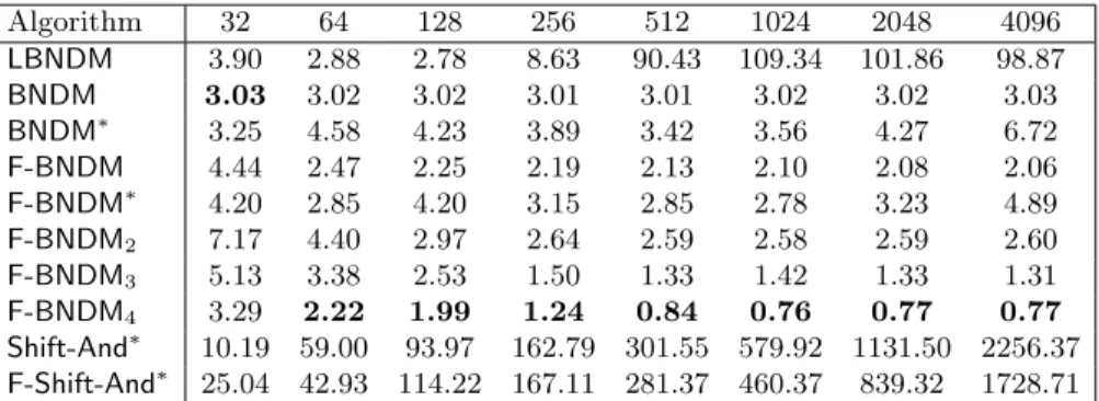
Algorithm 32 64 128 256 512 1024 2048 4096 LBNDM 2.44 1.46 1.13 0.77 0.62 0.55 1.94 10.81 BNDM 2.30 2.33 2.35 2.34 2.35 2.34 2.33 2.33 BNDM∗ 2.44 2.77 2.38 2.21 2.05 2.25 2.91 5.40 F-BNDM 2.44 1.62 1.27 1.03 1.03 0.99 0.98 0.93 F-BNDM∗ 2.53 1.64 1.23 1.72 1.49 1.50 1.60 2.44 F-BNDM2 3.26 2.24 1.63 1.04 0.68 0.67 0.68 0.68 F-BNDM3 2.49 1.61 1.26 0.84 0.59 0.55 0.55 0.56 F-BNDM4 2.29 1.37 1.05 0.70 0.53 0.51 0.57 0.58 Shift-And∗ 8.85 51.45 98.42 142.27 264.21 508.71 997.19 1976.09 F-Shift-And∗ 22.20 22.20 22.21 92.58 147.79 213.70 354.32 662.06 Table 3.1: Running times (ms) on the King James version of the Bible (σ = 63).
Algorithm 32 64 128 256 512 1024 2048 4096 LBNDM 1.24 0.84 0.60 0.48 0.38 0.52 7.83 36.84 BNDM 1.34 1.35 1.37 1.37 1.36 1.34 1.36 1.36 BNDM∗ 1.39 1.48 1.22 1.22 1.12 1.25 1.80 4.18 F-BNDM 1.19 0.77 0.56 0.49 0.48 0.48 0.48 0.47 F-BNDM∗ 1.36 0.84 0.83 0.89 0.77 0.79 1.00 1.92 F-BNDM2 1.42 0.96 0.67 0.48 0.35 0.35 0.36 0.36 F-BNDM3 1.26 0.71 0.47 0.32 0.32 0.40 0.63 0.76 F-BNDM4 1.36 0.71 0.45 0.30 0.30 0.40 0.73 2.92 Shift-And∗ 6.33 38.41 70.59 104.42 189.16 362.83 713.87 1413.76 F-Shift-And∗ 15.72 15.70 40.75 73.59 108.33 170.52 290.24 541.53 Table 3.2: Running times (ms) on a protein sequence of the Saccharomyces cerevisiae genome (σ = 20).
than w, as our encoding allows to pack more state configurations per bit on the average as shown in a table below. In the multi-word variants, the shift lengths for both algorithms, denoted BNDM∗ and F-BNDM∗, are always equal, as they
use the same automaton; however, the 1-factorization based encoding involves a smaller number of words on the average, especially for long patterns, thus providing a considerable speedup.
The tests have been performed on a 2.33 GHz Intel Core 2 Duo. We used the input files (i), (iii), (iv) (see Section 2.6).
For each input file, we have generated sets of 100 patterns of fixed length m randomly extracted from the text, for m ranging over the values 32, 64, 128, 256, 512, 1024, 2048, 4096. For each set of patterns we report the mean over the running times of 100 runs.
Algorithm 32 64 128 256 512 1024 2048 4096 LBNDM 3.90 2.88 2.78 8.63 90.43 109.34 101.86 98.87 BNDM 3.03 3.02 3.02 3.01 3.01 3.02 3.02 3.03 BNDM∗ 3.25 4.58 4.23 3.89 3.42 3.56 4.27 6.72 F-BNDM 4.44 2.47 2.25 2.19 2.13 2.10 2.08 2.06 F-BNDM∗ 4.20 2.85 4.20 3.15 2.85 2.78 3.23 4.89 F-BNDM2 7.17 4.40 2.97 2.64 2.59 2.58 2.59 2.60 F-BNDM3 5.13 3.38 2.53 1.50 1.33 1.42 1.33 1.31 F-BNDM4 3.29 2.22 1.99 1.24 0.84 0.76 0.77 0.77 Shift-And∗ 10.19 59.00 93.97 162.79 301.55 579.92 1131.50 2256.37 F-Shift-And∗ 25.04 42.93 114.22 167.11 281.37 460.37 839.32 1728.71 Table 3.3: Running times (ms) on a DNA sequence of the Escherichia coli genome (σ = 4).
(A) ecoli protein bible
32 32 32 32 64 63 64 64 128 72 122 128 256 74 148 163 512 77 160 169 1024 79 168 173 1536 80 173 176 2048 80 174 178 4096 82 179 182
(B) ecoli protein bible
32 15 8 6 64 29 14 12 128 59 31 26 256 119 60 50 512 236 116 102 1024 472 236 204 1536 705 355 304 2048 944 473 407 4096 1882 951 813
(C) ecoli protein bible
32 2.13 4.00 5.33 64 2.20 4.57 5.33 128 2.16 4.12 4.92 256 2.15 4.26 5.12 512 2.16 4.41 5.01 1024 2.16 4.33 5.01 1536 2.17 4.32 5.05 2048 2.16 4.32 5.03 4096 2.17 4.30 5.03
Table 3.4: (A) The length of the longest substring of the pattern fitting in w bits; (B) the size of the minimal 1-factorization of the pattern; (C) the ratio between m and the size of the minimal 1-factorization of the pattern.