SCIENZE DELL'INGEGNERIA CIVILE
_____________________________________________________
SCUOLA DOTTORALE / DOTTORATO DI RICERCA IN
XXVIII
______________________
CICLO DEL CORSO DI DOTTORATO
DEFINITION OF SEISMIC INPUT FOR STRUCTURAL
SAFETY EVALUATION. TWO CASE STUDIES:
Seismic response of concrete dams; dynamic soil-structure
interaction of the Leaning Tower of Pisa
__________________________________________________
Titolo della tesi
Dott.Ing. Gabriele Fiorentino
__________________________
__________________
Nome e Cognome del dottorando
firmaProf. Camillo Nuti
_________________________
__________________
Docente Guida/Tutor: Prof.
firmaProf. Aldo Fiori
________________________
__________________
Collana delle tesi di Dottorato di Ricerca In Scienze dell’Ingegneria Civile
Università degli Studi Roma Tre Tesi n° 58
La definizione dell'input sismico è un punto fondamentale per la valutazione della risposta dinamica delle strutture. Strutture strategiche quali le dighe o edifici monumentali che fanno parte del patrimonio architettonico necessitano che l'input sismico venga valutato con uno studio ad hoc, specialmente per un territorio caratterizzato da una sismicità medio-alta quale quello italiano. Nella presente tesi di dottorato viene presentato un metodo "ibrido" per la valutazione della pericolosità sismica, attraverso il quale combinando i tradizionali approcci probabilistico e deterministico si ottiene un terremoto di scenario. I parametri geofisici di questo evento sismico vengono quindi utilizzati per la selezione di accelerogrammi spettro-compatibili. La procedura proposta è stata quindi applicata a due casi studio di riferimento: nel primo caso a due dighe in calcestruzzo, per le quali è stata calcolata la risposta dinamica con un approccio step-by-step, partendo da analisi semplificate di scorrimento alla base fino ad arrivare ad analisi accurate in 3D con la valutazione del danno atteso. Nel secondo caso è stata valutata la risposta dinamica della Torre pendente di Pisa, dapprima analizzando gli studi esistenti ed individuandone le criticità, quindi definendo l'input sismico alla base tenendo in considerazione l'interazione suolo-struttura e le prove geofisiche eseguite nella Piazza dei Miracoli.
Abstract
The definition of the seismic input is an essential step for the evaluation of the dynamic response of structures. Strategic structures like dams or monumental buildings which are part of the architectural heritage require a specific study in order to evaluate the seismic input, especially in a country with medium-high seismicity like Italy. This work uses a hybrid approach for the evaluation of the seismic hazard, by matching the probabilistic and deterministic methods in order to obtain a controlling earthquake. The geophysical parameters of this event are then used for the selection and adjustment of spectrum-compatible accelerograms. The procedure is applied to two case studies: the first is represented by two concrete dams, for which the dynamic response is evaluated through a step-by-step method: starting from simplified analyses to obtain dam base sliding to more accurate analyses which can allow an estimate of the expected damage on the structure. The second case study the dynamic response of the Leaning Tower of Pisa is assessed, first through an identification of the critical issues in the existing studies on the topic, then by defining the seismic input considering soil-structure interaction and the recent geophysical tests performed in the Square of Miracles.
Contents
FIGURES INDEX ... XI TABLES INDEX ...XXII
1 INTRODUCTION ... 1
1.1 AIM OF THE STUDY ... 1
1.2 THESIS LAYOUT ... 3
PART I - DEFINITION OF SEISMIC INPUT ... 5
2 SEISMIC RISK AND STRUCTURES ... 5
2.1 SEISMIC RISK ... 5
2.2 SEISMIC RISK IN ITALY ... 9
2.3 SEISMIC HAZARD AND STRATEGIC STRUCTURES ... 9
2.4 SEISMIC HAZARD AND ARCHITECTURAL HERITAGE ... 12
3 PROCEDURE TO EVALUATE SEISMIC INPUT ... 19
3.1 INTRODUCTION ... 19
3.2 PSHA VS DSHA- HYBRID APPROACH ... 22
3.3 PROBABILISTIC SEISMIC HAZARD ASSESSMENT ... 24
3.4 CRISIS2014 PROCEDURE ... 49
3.5 SEISMIC HAZARD MODELS FOR ITALY:MPS04-S1 AND SHARE PROJECT ... 50
3.6 DISAGGREGATION ... 54
3.8 VERTICAL SPECTRA AND V/H RATIO ... 64
4 SELECTION OF ACCELEROGRAMS ... 67
4.1 THE FINAL STEP OF HYBRID APPROACH ... 67
4.2 SEISMIC CODES REQUIREMENTS ... 72
4.3 SCALING REAL ACCELEROGRAMS ... 73
4.4 SPECTRAL MATCHING ... 82
PART II - SEISMIC RESPONSE OF CONCRETE DAMS ... 85
5 INTRODUCTION ... 85
5.1 ITALIAN CODE DAMS CLASSIFICATION ... 88
5.2 ITALIAN CODE SEISMIC REQUIREMENTS ... 90
5.3 ICOLDBULLETIN 148 ... 93
5.4 SELECTION OF A RETURN PERIOD ... 97
6 DEFINITION OF SEISMIC INPUT ... 98
6.1 EVALUATION OF SEISMIC HAZARD FOR 4 SITES ... 98
6.2 ANALYSIS OF THE SEISMICITY OF THE SITES ... 99
6.3 UNIFORM HAZARD SPECTRA ... 107
6.4 DISAGGREGATION ... 112
6.5 SCENARIO EARTHQUAKES (DSHA) ... 118
6.6 SETS OF SCALED AND MATCHED ACCELEROGRAMS ... 121
7 SIMPLIFIED ANALYSES - EVALUATION OF BASE SLIDING ... 125
7.2 BASE SLIDING:NUTI-BASILI METHOD (2009) ... 131
7.3 APPLICATION OF THE METHOD TO A CASE STUDY ... 135
8 SAFEDAM ... 146
8.1 A PROBABILISTIC PROGRAM TO EVALUATE DAM BASE SLIDING ... 146
8.2 SELECTION OF RANDOM VARIABLES ... 147
8.3 EQUIVALENT STATIC ANALYSIS ... 148
8.4 DYNAMIC ANALYSES ... 151
8.5 APPLICATION TO THE CASE STUDY ... 152
8.6 CONSIDERATIONS ... 154
9 ACCURATE ANALYSES ... 156
9.1 CASE STUDIES... 157
9.2 FINITE ELEMENT MODEL ... 158
9.3 PRE-SEISMIC STATE ... 164
9.4 LINEAR ANALYSES... 167
9.5 CHOICE OF ACCELERATION TIME HISTORIES ... 168
9.6 DISPLACEMENT TIME HISTORIES COMPARISON ... 169
9.7 EXPECTED DAMAGE ... 171
PART III - DYNAMIC SOIL-STRUCTURE INTERACTION OF THE LEANING TOWER OF PISA... 179
10 INTRODUCTION ... 179
10.2 GEOMETRY OF THE TOWER ... 182
10.3 ITALIAN GUIDELINES - REDUCTION OF RISK OF CULTURAL HERITAGE ... 183
10.4 SEISMIC SAFETY ASSESSMENT ACCORDING TO ITALIAN GUIDELINES ... 184
11 PAST STUDIES ON THE SEISMIC RESPONSE OF THE TOWER ... 186
11.1 GRANDORI &FACCIOLI (1993) ... 186
11.2 ISMES(1995) ... 188
11.3 MACCHI &GHELFI (2006) ... 192
12 GEOPHYSICAL TESTS ... 193
12.1 THE GROUND UNDERLYING THE TOWER ... 193
12.2 EXISTING TESTS ... 194
12.3 AMBIENT VIBRATION TESTS ... 197
13 FOUNDATION GEOMETRY AND MODEL... 213
13.1 INTRODUCTION ... 213
13.2 SOIL-STRUCTURE INTERACTION ... 217
13.3 EXPERIMENTAL MODAL FREQUENCIES ... 218
13.4 SHEAR MODULUS AT SMALL DEFORMATIONS ... 223
13.5 WOLF FORMULATION ... 223
13.6 EVALUATION OF DYNAMIC IMPEDANCES ... 228
14 MODAL ANALYSIS ... 230
14.1 SIMPLIFIED MODEL (SAP2000) ... 230
14.3 MODAL SHAPES ... 232
14.4 MODEL UPDATING ... 235
15 SEISMIC INTENSITIES EXPECTED IN PISA ... 238
15.1 GRANDORI &FACCIOLI (1993) ... 238
15.2 SCENARIO EARTHQUAKES ... 240
15.3 SELECTION OF ACCELEROGRAMS ... 250
16 SITE RESPONSE ANALYSIS ... 255
16.1 INTRODUCTION ... 255
16.2 DECAY CURVES ... 257
16.3 ANALYSIS RESULTS ... 259
17 DYNAMIC RESPONSE OF THE TOWER ... 262
17.1 TYPE OF ANALYSIS AND RESULTS ... 262
18 CONCLUSIONS ... 264
Figures index
Fig. 2.1 Number of deaths caused by earthquakes in 2012 (Daniell, 2012) 5
Fig. 2.2 Direct economic losses in each 2012 CATDAT earthquake (Daniell,
2012) 6
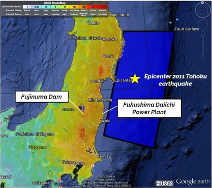
Fig. 2.3 Map of Fujinuma Dam, Fukushima Nuclear Power Plant and the epicenter of the earthquake with MCS intensities (modified from USGS, 2016) 10
Fig. 2.4 Collapse of Fujinuma dam, Japan 2011 11
Fig. 2.5 Collapse of the frescoed vaults in Assisi, 1997 13
Fig. 2.6 Bell Tower of Nocera Umbra cathedral: after collapse (left) after
reconstruction (right) 13
Fig. 2.7 Collapse of the Dome of the Church of Anime Sante: Before (left) and
after the earthquake (right) 14
Fig. 2.8 Collapse of the facade of the Town Hall of Sant'Agostino, May 2012 15 Fig. 2.9 Collapse of the Bell Tower of Novi (Modena), Before the earthquake
(left) and after (right) 16
Fig. 3.1 Proposed procedure to define seismic input 19
Fig. 3.2 ZS9 Seismogenic zoning for Italian territory (Meletti et al. 2008) 27
Fig. 3.3 Hazard curves depending on seismic sources considered 28
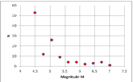
Fig. 3.4 Number of earthquake vs Magnitude for Zone 923 30
Fig. 3.5 Gutenberg- Richter relation for zone 923 30
Fig. 3.6 Comparison between GMPEs for Mw 6 and spectral period T=0,1 s 40
Fig. 3.8 Comparison between deterministic spectra for Mw 6, R=10 km 41
Fig. 3.9 Comparison between deterministic spectra for Mw 6, R=50 km 41
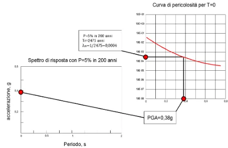
Fig. 3.10 PGA Hazard Curve 43
Fig. 3.11 Hazard Curve for structural period T=0,2 s 44
Fig. 3.12 Expected PGA for Italy, P=10% in 50 years (TR=475 years) (INGV) 45
Fig. 3.13 Expected PGA for Site C, TR=475 years (INGV) 46
Fig. 3.14 Site C: Elastic Horizontal response spectrum (NTC 2008), TR=475
years 47
Fig. 3.15 475 years Uniform Hazard Spectra for Site C 48
Fig. 3.16 NTC08 and MPS04 response spectra for different TR (NTC 2008) 51
Fig. 3.17 Seismic Hazard Maps fpr PGA from MPS04 and SHARE (Meletti
2014) 53
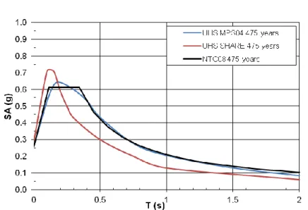
Fig. 3.18 Comparison: NTC08 spectrum and UHS from MPS04 and SHARE 54
Fig. 3.19 Disaggregation for PSA=0,59 g, T=0,1 s 57
Fig. 3.20 Contribution to hazard by Magnitude M for PSA, T=0,1 s 58
Fig. 3.21 Contribution to hazard by Distance R for PSA, T=0,1 s 58
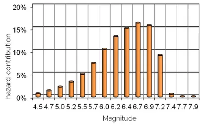
Fig. 3.22 Disaggregation for PSA=0,35 g, T=1 s 59
Fig. 3.23 Contribution to hazard by Magnitude M for PSA, T=1 s 59
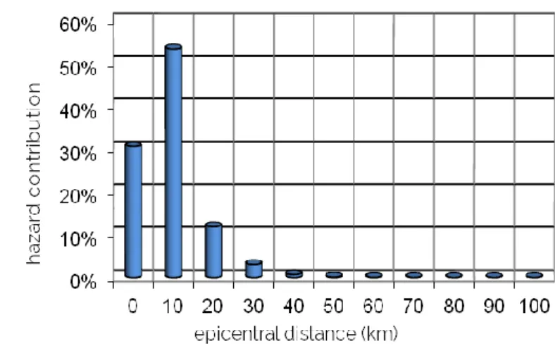
Fig. 3.24 Contribution to hazard by Distance R for PSA, T=1 s 60
Fig. 3.25 Controlling earthquakes for site C - 475 years 62
Fig. 3.26 Comparison between UHS and deterministic spectra - SP96 63
Fig. 3.28 Effect of soil condition on V/H ratio - SP96 GMPE 65 Fig. 4.1 Evaluation of an artificial accelerogram with Belfagor (Mucciarelli,
2004) 69
Fig. 4.2 Main window of the software REXEL (Iervolino, 2010) 78
Fig. 4.3 Main window of In-Spector (Acunzo, 2014) 80
Fig. 4.4 Main window of Seismomatch ( 83
Fig. 5.1 Classification of worldwide dams by purpose (ICOLD) 85
Fig. 5.2 Classification of worldwide dams by dam type (ICOLD) 86
Fig. 5.3 Map of existing Large Dams in Italy (ITCOLD) 87
Fig. 5.4 Example of gravity dam 88
Fig. 5.5 Example of arch dam 89
Fig. 5.6 Example of arch-gravity dam 90
Fig. 6.1 Four Italian Dam sites selected for Seismic Hazard Assessment 98
Fig. 6.2 Composite and individual seismogenic sources for Site A, Piemonte 100 Fig. 6.3 Seismogenic zones; historical and instrumental seismicity for Site A 101 Fig. 6.4 Composite and individual seismogenic sources for Site B, Toscana 102 Fig. 6.5 Seismogenic zones; historical and instrumental seismicity for Site B 102 Fig. 6.6 Composite and individual seismogenic sources for Site C, Abruzzo 103 Fig. 6.7 Seismogenic zones; historical and instrumental seismicity for Site C 104 Fig. 6.8 Composite and individual seismogenic sources for Site D, Calabria 105 Fig. 6.9 Seismogenic zones; historical and instrumental seismicity for Site D 106
Fig. 6.10 Geographical coordinates and seismogenic zoning ZS9 in CRISIS
2014 107
Fig. 6.11 Definition of recurrence relation parameters in CRISIS 2014 108
Fig. 6.12 Definition of GMPE in CRISIS 2014 108
Fig. 6.13 Probabilistic response spectra for site A 110
Fig. 6.14 Probabilistic response spectra for site B 110
Fig. 6.15 Probabilistic response spectra for site C 111
Fig. 6.16 Probabilistic response spectra for site D 111
Fig. 6.17 Disaggregation for Site A: PGA (top), PSA 0,2s (middle), PSA 1s
(bottom) 114
Fig. 6.18 Disaggregation for Site B: PGA (top), PSA 0,2s (middle), PSA 1s
(bottom) 115
Fig. 6.19 Disaggregation for Site C: PGA (top), PSA 0,2s (middle), PSA 1s
(bottom) 116
Fig. 6.20 Disaggregation for Site D: PGA (top), PSA 0,2s (middle), PSA 1s
(bottom) 117
Fig. 6.21 Comparison probabilistic/deterministic spectra for site A 119
Fig. 6.22 Comparison probabilistic/deterministic spectra for site B 120
Fig. 6.23 Comparison probabilistic/deterministic spectra for site C 120
Fig. 6.24 Comparison probabilistic/deterministic spectra for site D 121
Fig. 6.25 Site D: response spectra of the accelerograms scaled with REXEL 122 Fig. 6.26 Site D: response spectra of the accelerograms modified with
Fig. 6.27 Comparison between scaled and matched accelerogram #6335 124
Fig. 7.1 Dam-reservoir dynamic interaction according to Westergaard 127
Fig. 7.2 Fenves and Chopra method: Dam-reservoir interaction 128
Fig. 7.3 Fenves and Chopra method: Dam-foundation interaction 130
Fig. 7.4 Nuti-Basili model for SDOF non-linear system (Nuti and Basili, 2009) 133 Fig. 7.5 Plot of μ vs β as presented by Nuti and Basili (Nuti and Basili, 2009) 135 Fig. 7.6 Highest block of the gravity dam (left) and simplified model (right) 136
Fig. 7.7 SDOF equivalent system proposed by Nuti and Basili (2009). 137
Fig. 7.8 SDOF system modeled in Opensees 137
Fig. 7.9 Response for the accelerogram 006335: (top) relative displacement of nonlinear SDOF compared with a linear one; (bottom) plot of the base sliding.
139 Fig. 7.10 Base displacement obtained with the 56 analyses for sites A, B, C, D 140
Fig. 7.11 β-μ points compared with the Nuti and Basili correlation curve. 144
Fig. 8.1 Relative frequency of Sliding Safety Factors 151
Fig. 8.2 Equivalent linear and non-linear response (top), residual base sliding
(bottom) 152
Fig. 8.3 Synthetic results of equivalent static analyses 153
Fig. 8.4 Synthetic results of dynamic analyses 154
Fig. 9.2 Front view of the arch-gravity dam 158
Fig. 9.3 Finite element model of the gravity dam 159
Fig. 9.4 Finite element model of the arch-gravity dam 159
Fig. 9.5 Model of the gravity dam including the foundation 162
Fig. 9.6 Model of the arch-gravity dam including the foundation 162
Fig. 9.7 Reservoir model for arch gravity dam in Abaqus 163
Fig. 9.8 Winter (left) and summer (right) thermal effects for the arch-gravity
dam 165
Fig. 9.9 Pre-seismic state for the gravity dam 166
Fig. 9.10 Pre-seismic state for the arch-gravity dam 167
Fig. 9.11 Selected accelerograms for accurate analyses 169
Fig. 9.12 Crest Displacement time histories for central block of gravity dam 170 Fig. 9.13 Crest Displacement time histories for central block of arch-gravity
dam 170
Fig. 9.14 Tensional (a) and compressive (b) behavior of the material (Lee and
Fenves, 1998) 172
Fig. 9.15 Damage on the gravity dam - Site A: DS wall (top) and US wall
(bottom) 174
Fig. 9.16 Damage on the gravity dam - Site D: DS wall (top) and US wall
(bottom) 175
Fig. 9.17 Damage on the arch-gravity dam - Site A: DS wall (top) and US wall
Fig. 9.18 Damage on the arch-gravity dam - Site D: DS wall (top) and US wall
(bottom) 177
Fig. 10.1 History of the inclination of the Tower (Burland 2009) 179
Fig. 10.2 Intervention of under-excavation under the Tower (Burland 2009) 180
Fig. 10.3 Elevation and section of the Tower, N-S direction ([74][79]) 182
Fig. 11.1 Finite element model (Grandori e Faccioli 1993) 187
Fig. 11.2 Vibrodyne used by ISMES for the test (1995) 189
Fig. 11.3 Modal shapes obtained by ISMES (1995) 190
Fig. 11.4 Finite element model built by ISMES (1995) 191
Fig. 12.1 Soil profile of the ground underlying the Tower (Burland, 1994) 194
Fig. 12.2 Comparison of Vs obtained with geophysical tests in the last 25 years 195
Fig. 12.3 Propagation of body waves in a linear elastic medium 197
Fig. 12.4 Propagation of surface waves in a linear elastic medium 198
Fig. 12.5 Geometric dispersion of Rayleigh waves (Foti et al. 2015) 199
Fig. 12.6 Inverse problem (modified from Foti et al. 2015) 201
Fig. 12.7 Acquisition system for the Array 2D test 202
Fig. 12.8 Array 2D test performed in the Square of Miracles, November 2015 203
Fig. 12.9 installation of a seismic station close to the Tower 203
Fig. 12.11 Array Transfer function (left) and experimental dispersion curve
(right) 206
Fig. 12.12 Soil profile and dispersion curve obtained with Geopsy 207
Fig. 12.13 Comparison between geophysical tests including Array 2D results 208
Fig. 12.14 H/V test performed in the Square of Miracles, November 2015 210
Fig. 12.15 Fourier spectra of records (left) Directionality of passive sources
(right) 210
Fig. 12.16 Resonance peaks of H/V spectral curve for a single station 211
Fig. 13.1 Section of foundation ring (Burland 1994) 213
Fig. 13.2 Condition of the basement of the Tower before the works by
Gherardesca (1838) 214
Fig. 13.3 Works for the consolidation of the Catino 215
Fig. 13.4 Connection between the foundation and the Catino (Burland, 2009)216
Fig. 13.5 Fondazione della torre e catino di base, configurazione attuale 216
Fig. 13.6 Schematization of soil-structure interaction (Mylonakis, 2006) 217
Fig. 13.7 Position of the sensors on the Tower (left) and on the ground (right) 219
Fig. 13.8 Response recorded on the Tower by sensors S1, S2, S3 220
Fig. 13.9 CWT of the recorded tower response 221
Fig. 13.10 Vertical response due to the vertical mode (Filter 2-4 Hz) 222
Fig. 13.11 Vertical response due to the bending mode (Filter 0,8-1,2 Hz) 222
Fig. 13.13 Parameters of spring-dashpot-mass model (Wolf, 1994) 224
Fig. 13.14 Plot of k(a0) vs a0 - Horizontal translation 226
Fig. 13.15 Plot of k(a0) vs a0 - Vertical translation 226
Fig. 13.16 Plot of k(a0) vs a0 - Rocking 227
Fig. 13.17 Plot of k(a0) vs a0 - Torsion 227
Fig. 14.1 Scheme of the FE model 231
Fig. 14.2 First modal shape - Horizontal, direction E-W 233
Fig. 14.3 Second modal shape - Horizontal, direction N-S 234
Fig. 14.4 Third modal shape - Vertical 234
Fig. 14.5 6th modal shape - torsional 235
Fig. 15.1 Correlation between PGA and MCS intensity (modified from Sabetta) 239
Fig. 15.2 Response spectrum obtained by Grandori e Faccioli (1993) 240
Fig. 15.3 1Uniform Hazard Spectra - 130 years return period 241
Fig. 15.4 Uniform Hazard Spectra - 500 years return period 241
Fig. 15.5 Disaggregation for PSA 1s, TR=130 years 243
Fig. 15.6 Disaggregation for PSA 0,3s, TR=130 years 243
Fig. 15.7 Disaggregation for PSA 1s, TR=500 years 244
Fig. 15.8 Disaggregation for PSA 0,3s, TR=500 years 244
Fig. 15.9 Gutenberg-Richter relation for zone ZS916 246
Fig. 15.11 Comparison between spectra - 500 years 247
Fig. 15.12 V/H ratio for the response spectra of the Scenario earthquakes 249
Fig. 15.13 Comparison Horizontal/vertical spectra - 130 years 249
Fig. 15.14 Comparison Horizontal/vertical spectra - 500 years 250
Fig. 15.15 Selected scaled accelerograms - Horizontal - TR=130 years 251
Fig. 15.16Selected scaled accelerograms - Vertical- TR=130 years 252
Fig. 15.17 Selected scaled accelerograms - Horizontal - TR=500 years 252
Fig. 15.18 Selected scaled accelerograms - Vertical - TR=500 years 253
Fig. 15.19 Acceleration Time history on rigid soil - CAG 254
Fig. 16.1 Source-to-site travel path of body waves (Kramer, 1994) 255
Fig. 16.2 Source-to-site travel path of body waves (Yoshida, 2015) 256
Fig. 16.3 G/G0 decay curve for Pisa clays 258
Fig. 16.4 D/γ curve for Pisa clays 259
Fig. 16.5 Non-linear amplification function 260
Fig. 16.6 Response spectra of the accelerograms at ground level - TR=500 yrs
261 Fig. 16.7 Ground surface time history acceleration - Event Umbria-Marche
CAG 261
Fig. 17.1 Acceleration time history of node 30 - Event Umbria-Marche CAG 263 Fig. 17.2 Displacement time history of node 30 - Event Umbria-Marche CAG 263
Tables index
Tab. 3.1 EC8 Site Classification ... 35 Tab. 3.2 Parameters of the considered GMPEs ... 39 Tab. 3.3 Controlling earthquakes based on disaggregation ... 62 Tab. 5.1 Definition of Design Earthquakes for SEE ... 95 Tab. 6.1 Case studies sites for the evaluation of seismic input ... 99 Tab. 6.2 Controlling earthquakes for the case studies ... 118 Tab. 6.3 Intervals of Magnitude and distance for REXEL ... 122 Tab. 7.1 Results of simplified analyses ... 141 Tab. 7.2 Statistical parameters of the base residual displacement for the different groups of signals ... 143 Tab. 11.1 Parametri terreno Grandori e Faccioli (1993) ... 186 Tab. 11.2 Caratteristiche meccaniche del modello (Grandori e Faccioli 1993) ... 188 Tab. 11.3 Numerical results by Grandori e Faccioli (1993) ... 188 Tab. 11.4 Results of dynamic test by ISMES (1995) ... 189 Tab. 11.5 Results obtained with two numerical models by ISMES ... 191 Tab. 11.6 Position of the centroids of each Ordine, after Macchi e Ghelfi (2002) ... 192 Tab. 12.1 Ranges of parameters to constraint the problem ... 206 Tab. 13.1 List of the considered seismic events. ... 220 Tab. 13.2 Comparison of results from different authors ... 221
Tab. 13.3 Values of k(a0) for the identified modes ... 228
Tab. 13.4 Values of the dynamic impedances (units: kN/m2) ... 229 Tab. 14.1 Comparison between numerical and experimental frequencies. ... 232 Tab. 14.2 Comparison between experimental frequencies and numerical results after model updating. ... 236 Tab. 14.3 Comparison between the results of numerical analyses by various authors ... 236 Tab. 15.1 Correlation between MCS intensity/TR/PGA ... 239
Tab. 15.2 Selection of controlling earthquakes ... 245 Tab. 15.3 Search parameters for ITACA database ... 250 Tab. 15.4 Parameters used for the scaled accelerograms - 130 years return period ... 253 Tab. 15.5 Parameters used for the scaled accelerograms - 500 years return period ... 254 Tab. 17.1 Maximum acceleration and displacement results - 8th Ordine ... 262
1.1
Aim of the study
Recent earthquakes occurred in different areas of the world highlighted the fragility of existing structures and infrastructures. Seismic risk is particularly high for some structures, as strategic structures like hospitals, electric power plants and dams whose collapse could result in a large number of casualties or high economic losses.
Another category of structures whose seismic risk has to be assessed carefully are architectural heritage buildings, First of all because of their historical and artistic value; and then because they are characterized by high fragility of the building itself or of the soil-foundation-structure system. They are often located in highly seismic areas.
For different reasons, for both categories Codes and guidelines, as well as the technical literature require to perform specific studies in certain conditions in order to define the seismic input at a given site. Today the most used methods to evaluate the Seismic Hazard at a site are the Probabilistic approach (PSHA) and the deterministic approach (DSHA). According to some authors, better results can be achieved combining together these two methods. This "hybrid" method can be used to select real acceleration time histories, which are scaled or adjusted in order to obtain spectrum-compatible records. There is a wide range of computer programs that help to obtain these time histories, which can be used to perform non-linear dynamic analyses on structures.
The aim of this research work is to discuss the application of this method to two real case studies providing seismic actions having a strong connection with the seismo-tectonic conditions of the sites under analysis. The majority of the existing concrete dams was designed and constructed following seismic design criteria which now are considered obsolete. For this reason they need to be re-assessed with analyses that take into account the most advanced numerical techniques and scientific methods. In this work the Seismic Hazard Assessment was performed at four sites
in Italy characterized by a different level of seismicity, then acceleration time histories were selected using two different methods. Initially, for each site a dynamic non-linear analysis was performed to evaluate the base displacement of a dam, modeled as a simplified SDOF system. Subsequently, a gravity dam and an arch-gravity dam were taken into account as case studies for applications. Both structures were studied by means of 3D models, performing non-linear dynamic analyses and evaluating the expected damage.
One of the purposes of this study is to show the importance of the procedure to assess the seismic hazard in the framework of a step-by-step approach for the evaluation of the seismic safety of dams. The process starts from simplified analyses which can be useful to perform a rapid analysis of damage, to then move to more complex analyses which can provide all the parameters needed to state whether a concrete dam is safe or not.
The seismic behavior including soil-foundation-structure interaction of the Leaning Tower of Pisa was object of studies that date back to the end of the 20th century. The foundation of the Tower was consolidated from 1999 to 2001 by means of under-excavation, and the circular ring at the base known as "Catino" was rigidly connected to the foundation, so the boundary conditions of the foundation are changed. For these reasons it was necessary a study to evaluate the dynamic behavior of the Tower. First the hybrid method for the evaluation of the Seismic Hazard was applied to the site of the Square of Miracles in Pisa, in order to obtain the seismic input in terms of response spectra and accelerograms.
According to the Italian Guidelines on cultural heritage, for monuments like the Tower of Pisa a specific seismic hazard assessment has to be
performed. This should take into account the site's specific geologic and geotechnical conditions.
A modal analysis along with a sensitivity analysis was performed to find the modal frequencies of the Tower. These were then compared with the experimental ones while a model updating of the frequencies was done. In the Square of Miracles in Pisa the soft soil layers underlying the square have a great influence on the amplification of the ground motion. The study of the geophysical tests conducted in the past years and the execution of an Array 2D test performed in November 2015 gave the possibility to create a dynamic profile of the ground up to a depth of 100 meters, and to obtain the motion at the ground level, which was applied on the Tower to evaluate its dynamic response.
1.2
Thesis layout
This work is divided into three parts: in the first part, formed by chapters 2 to 4, the proposed procedure for defining the seismic input is discussed. Chapter 2 contains an introduction on the seismic risk for strategic structures and architectural heritage. Chapter 3 gives a brief overview of the method used, Chapter 4 introduces the hybrid approach to define response spectra and the description of the methods used to select accelerograms.
The second part of the thesis, from chapter 5 to 9, contains the application of the hybrid approach to two concrete dams. Chapter 5 introduces the provisions of Italian Code and ICOLD Bulletin, in chapter 6 the seismic input in terms of response spectra and accelerograms is defined. Chapter 7 and 8 contain applications of the method to simplified analyses of dams with the purpose to evaluate dam base sliding. Finally, chapter 9
discusses the dynamic response of dams with accurate analyses (3D FEM models).
In the third part, from chapter 10 to 17, the assessment of the dynamic soil-structure interaction of the Leaning Tower of Pisa is discussed. Chapter 10 starts with an introduction on seismic Codes and on the history of the works made on the Tower. Chapter 11 investigates past studies on the seismic response of the Tower, while chapter 12 discusses the past and recent geophysical tests performed in the Square of Miracles. In chapters 13, and 14 is presented the study of the interaction between the soil and structure, the modal analysis and the results of the model updating, together with the results obtained from the analysis of experimental records. In chapter 15 the seismic input expected in Pisa is evaluated in terms of response spectra and accelerograms, while in chapters 16 and 17 the results of the site response analysis and of the dynamic response of the Tower are discussed.
Chapter 18 presents a final summary of the work done, some conclusive remarks and possible future developments.
PART I - DEFINITION OF SEISMIC INPUT
2 Seismic risk and structures
2.1
Seismic Risk
The great number of casualties due to earthquakes has highlighted the high fragility level of the existing structures and infrastructures. Earthquakes cause each year a mean annual death toll of 21.800 casualties worldwide. From 1975 to 2005 the number of disasters has increased by about 400%, also depending on the rise in the population and urbanization.
Fig. 2.1 Number of deaths caused by earthquakes in 2012 (Daniell, 2012) According to 2012 report by CATDAT, a database of the damaging earthquakes, the number of total fatalities occurred that year was between 690 and 727, a quite low number in comparison to the mean annual death toll. Another important fact is related to economic losses. According to [1] a median value of 20,24 billions USD was estimated as amount of the total direct economic losses worldwide.
The highest economic losses in 2012 in the world were caused by the Emilia-Romagna earthquakes (M 5,8 and M 6) occurred in May 2012, with a median value of 17,5 billion USD of direct losses (Fig. 2.2). This large amount of losses is due mainly to two causes:
1. Earthquakes occurred in a highly industrialized area, which is characterized by a high density of factories and industrial plants. 2. The region had little to no seismic zoning under the Italian Codes
until 2003. Therefore the majority of industrial plants were built without using appropriate design details against earthquakes.
Fig. 2.2 Direct economic losses in each 2012 CATDAT earthquake (Daniell, 2012) 2.1.1 Definition of seismic risk
The definition of Risk and Hazard are often confused with each other, but it could easily be recognized that between these two concepts there is a cause and effect relationship, as indicated for example in [2]. Hazard could be an event which has the potential to create loss. Conversely, Risk
depends on the actual exposure of something which has a human value. The Risk can be evaluated as the combination of the probability of an hazardous event and its negative consequences.
According to these definitions, Seismic Risk is defined as the amount of damage expected at a given site as a consequence of a seismic event in a given time period, depending on the seismicity of an area, on the resistance of buildings and on anthropization. The traditional form to express the seismic risk is:
E V H
R Where:
‒ H is the Seismic Hazard ‒ V is the Vulnerability ‒ E is the Exposure
Since it is not possible to act on the Hazard and the Exposure, the reduction of seismic Risk is generally performed by reducing the vulnerability of buildings during construction or by retrofitting the existing structures. Another issue is to reduce the probability of damages due to secondary hazards, such as landslides, liquefaction or tsunamis triggered by the earthquake.
2.1.2 Seismic Hazard
The seismic hazard is defined as the probability of occurrence of a given level of seismic intensity at a given site in a defined time period. The seismic intensity can be expressed as local intensity (e.g. X degree of the MCS scale), magnitude or ground motion acceleration, and it represents a measure of the seismicity of an area.
As we will see in the next chapter, there are two approaches to evaluate the Seismic Hazard, namely the Probabilistic Seismic Hazard Assessment (PSHA) and the Deterministic Seismic Hazard Assessment (DSHA). 2.1.3 Vulnerability
The vulnerability is the capacity of buildings to report damages due to an earthquake. The collapse of buildings is the main cause of death during earthquakes.
The Italian Code, D.M. 14/1/2008 (NTC2008), gives prescriptions for the expected behavior of buildings for different levels of seismic intensity. A structure should not be damaged for a low level of seismicity, should not have structural damages for a medium level of seismicity and should not collapse for high seismicity levels, also if major damage can occur.
The vulnerability is the element of seismic risk which can be modified, increasing the resistance of existing constructions. In fact it is possible to lower the vulnerability of buildings with interventions which can improve their capacity to resist to earthquakes suffering minor damages.
2.1.4 Exposure
The exposure estimates the value of objects and people subject to the seismic action and therefore exposed to the seismic risk. For the system of civil protection one of the priorities in case of earthquake is the safeguard of human lives. For this reason it is very important to estimate the number of people involved in such an event, and to evaluate quickly the number of casualties.
This is a complex operation because the estimate depends on a great number of factors, as the type of buildings (residential, industrial, etc), the
hour of the earthquake (day, night), the possibility to hide or to escape somewhere.
In Italy, another aspect of the exposure is the presence of an incredible cultural heritage, formed by the built heritage of the historical centers of Italian cities and small towns.
2.2
Seismic risk in Italy
Italy is characterized by a medium-high level of seismicity (for frequency and intensity), in fact it is one of the European countries with the highest levels of seismicity, because it is placed at the boundary between the African and the Eurasian plates. The vulnerability is very high, due to a fragility of the built heritage, and a very high exposure due to very high density of population and the presence of a cultural, architectural and historical heritage which is unique in the world.
Therefore Italy is a country with a very high seismic risk in terms of victims, damages to the built heritage and direct and indirect costs expected after an earthquake.
2.3
Seismic Hazard and Strategic structures
The evaluation of the seismic hazard is especially important for strategic structures, whose collapse could cause very high damage to goods and a very high death toll. Some examples of strategic structures are highway bridges, nuclear power plants and large dams.
The 2011 Tohoku earthquake (Mw 9,1) was one of the largest and most
destructive seismic events of the last years. As it is well known the Tsunami caused the failure of the cooling system at the Fukushima Daiichi Nuclear Power Plant, resulting in an overheating of the nuclear
reactor and the raising of radiation levels inside (1.000 times the normal levels) and outside (8 times the normal levels) the plant.
With regard to dams, the same earthquake caused the collapse of an earth dam with a height of 18 meters, with a reservoir volume of 1,5 million m3 (See Fig. 2.4). The resulting flood destroyed the village of Naganuma, where 5 houses were washed away, and 8 people lost their lives, as it is reported in [4] and [6]. In the two months after the earthquake, approximately 400 dams were inspected in Japan, and the experts found that the structures had withstood severe ground motions and retained the water, as reported in [4], while minor or moderate damage was found.
Fig. 2.3 Map of Fujinuma Dam, Fukushima Nuclear Power Plant and the epicenter of the earthquake with MCS intensities (modified from USGS, 2016)
Fig. 2.3 shows the seismic intensity map of the East Coast of Japan, highlighting the positions of the Fujinuma ike Dam and of the Fukushima Nuclear Power Plant.
Until today there have been no collapses of concrete dams due to earthquakes, but some of these structures were seriously damaged, suffering from sliding at the base of the structure, joint opening, collapse of appurtenant structures.
Fig. 2.4 Collapse of Fujinuma dam, Japan 2011
Focusing on Large dams, it is possible to point out that both the recent guidelines of the Italian Code on Dams (2014) and ICOLD (International Committee On Large Dams), the international NGO which is a point of reference in the field on dam engineering, publishing bulletins and guidelines, recommend to evaluate the seismic input for Large dams with appropriate Seismic Hazard studies, instead of using standard Code Spectra.
In fact, as it will be described in sections 5.2 and 5.3, both require a specific seismic hazard evaluation for the dams whose collapse could cause a high risk for the community.
The intensity of the recommended seismic action is very high: For a collapse limit state the return period is:
‒ 2.500 years for a new dam and 1950 years for an existing dam according to the guidelines of the Italian Code.
‒ 10.000 years for ICOLD bulletin 148
It is then clear that the seismic hazard must be evaluated with an appropriate study, taking into account all the parameters which could influence the expected intensity at the site.
2.4
Seismic Hazard and Architectural heritage
Italy is the country which has the greatest number of UNESCO world heritage sites in the world, with a total of 47 sites including, as examples, the historic centre of Rome, Piazza del Duomo in Pisa, the city of Venice and its lagoon, and the archeological areas of Pompei (Campania) and Agrigento (Sicily), as reported in [7].It is straightforward that all these areas and monuments have an extraordinary value, which has to be protected from anthropic, environmental and natural risks. Meanwhile, earthquakes produce great damages to the cultural heritage due to the high level of seismic hazard, together with the fragility which characterizes old masonry constructions, and in particular vaults and domes, high structures such as clock and bell towers, pitched roofs, tympanums and apses of churches.
A recent work by Parisi and Augenti [8] summarizes the damages caused by recent earthquakes in Italy and in the rest of the world.
Fig. 2.5 Collapse of the frescoed vaults in Assisi, 1997
Fig. 2.6 Bell Tower of Nocera Umbra cathedral: after collapse (left) after reconstruction (right)
In the last twenty years, three earthquakes in Italy caused a great number of casualties and major damage to the cultural heritage. From May 1997 to April 1998 an earthquake cluster (Mw 5,7-6) hit the regions of Umbria
and Marche, causing 11 casualties, and damaging important monuments. The largest number of deaths and damages had been in the villages of Cesi, Collecurti, Montesanto, Annifo Villa. In Assisi the dome of the upper Basilica of San Francesco collapsed, causing the death of 4 people and the damage of the vaults, some painted by Giotto and Cimabue (See Fig. 2.5). In Nocera Umbra there were several damages in the historical centre, where the bell tower collapsed (See Fig. 2.6). Only in Umbria a total of 2316 monumental buildings were damaged.
The 2009 L'Aquila earthquake came after a sequence of tremors lasting from January to March, beginning with the Mw 6,3 mainshock on April
6th. The sequence caused 308 deaths and 1600 injured. Over 80.000 buildings were inspected and 30,6% of them were found to be unfit for use. Experts checked 1800 monumental constructions, 55,1% of them were strongly damaged or collapsed. Many others historical buildings, such as the church Basilica di Santa Maria di Collemaggio and the Church of the Anime Sante (See Fig. 2.7).
Fig. 2.7 Collapse of the Dome of the Church of Anime Sante: Before (left) and after the earthquake (right)
Today, while the majority of the modern buildings of the town have been reconstructed, and the 55% of the private buildings of the historical centre was reconstruct or consolidated, as the reconstruction of public buildings is extremely slow, as reported in [10].
The 2012 Emilia-Romagna earthquakes were a series of seismic events which took place from May to June, with seven events with Mw > 5.0.
Two mainshocks hit the area on 20 and 29 May, causing respectively 7 and 19 casualties, 350 injured, 14.000 homeless people and heavy damage to industrial and historic buildings.
The maximum values for horizontal and vertical PGA were recorded as 0,26g and 0,31g. These earthquakes caused the interruption of business activities in the epicentral area, because of the high level of damage of the industrial plants. While 20 May event had a moderate impact on the
Fig. 2.9 Collapse of the Bell Tower of Novi (Modena), Before the earthquake (left) and after (right)
cultural heritage, 29 May event caused major damage to historical buildings. Two examples of buildings damaged by the earthquake are the Town Hall of Sant'Agostino, in the province of Ferrara (See Fig. 2.8) and the partial collapse of the Bell Tower of Novi, in the province of Modena. From the experiences of the events of Umbria-Marche (1997-1998) and L'Aquila (2009) it was clear that the evaluation of seismic risk for historical structures has many differences from the assessment of modern structures. In fact, for modern structures the current approach is to consider a seismic input with a probability of occurrence of 10% in 50 years, the normal reference period for a civil construction, resulting in a return period of the seismic action of 475 years.
Considering such a return period could not be appropriate for historical buildings, because the concepts included in the Codes are based mainly on modern structures, while historical buildings are generally built
following criteria which are not based on the principles of the materials and structure mechanics, but on proportions and building techniques known as Regole dell'Arte, which were based on past building experiences, intuition and a great knowledge of the materials used. Many of these structures are made of old masonry, which can be particularly weak for seismic actions. Therefore, retrofit solutions for these buildings have to be designed carefully, trying to find a balance between earthquake protection and life safety and the conservation of the cultural heritage. There are other factors to take into account for historical buildings, as reported in [9]. For example it is possible that buildings with great architectural or historical value could be rarely used. In this case it can be necessary to prevent the collapse of the structure, while life safety and immediate use of the building are not a priority. Otherwise, there are structures with a minor importance which can be public buildings, for which life safety and immediate use are necessary.
In [9] the authors proposed a method to define seismic input, evaluating Code response spectra by dividing the usual return period (i.e. 475 years) for some coefficients γ ranging from 0,5 to 2, increasing or decreasing the seismic input. This factors are function of the intended use of the building, its historical and architectural value.
In 2011 the Italian Government proposed a Directive which contained the guidelines for the "Evaluation and the reduction of the seismic risk for the cultural heritage" [11], referring to the existing Italian Code. In presence of soft heterogeneous soil, and depending on the different stiffness and continuity of shallow soil layers, and on topographic discontinuities there may be ground motion amplification effects, both in terms of maximum accelerations and frequency content.
In this document it is stated that in these cases it is necessary to perform specific analyses of local seismic response, taking into account the available studies on local seismic response and micro-zoning.
If conversely the stratigraphic and topographic conditions fall in the categories described in paragraph 3.2.2 of Italian Code [12], it is possible to use the response spectra defined by the Code.
3 Procedure to evaluate seismic input
3.1
Introduction
Aim of the procedure used in this work is to define the seismic input, first in terms of response spectrum, then in terms of acceleration time histories, which are useful to perform nonlinear dynamic analyses. A flowchart of this procedure is displayed in Fig. 3.1.
The procedure starts with the assessment of a Uniform Hazard Spectrum on rigid soil, which can be evaluated through a Probabilistic Seismic Hazard Assessment, or taken by the Code. In order to evaluate UHS it is necessary to choose an appropriate Return Period TR, corresponding to a
given probability of exceedance of the ground motion intensity level in a given reference period. The PSHA and the Code spectra can be compared to see if there is consistency.
As we will see, the Uniform Hazard Spectra include the contribution to the Hazard of all the sources involved in calculations. Therefore, they provide no information about earthquakes which have produced the spectral accelerations. Disaggregation of the Hazard allows to obtain the M-R combinations which are more likely to produce the expected level of ground motion intensity at the site for a given spectral period, depending on the structure that has to be analyzed.
The disaggregation of the hazard has to be validated by means of a comparison with the historical seismicity of the area of interest, which is generally synthesized in seismic catalogues that include all the historical earthquakes in a certain region.
Searching in the seismic catalogue, which can be reported in a GIS map, one or more Scenario earthquakes can be selected. The Magnitude and the Distance of the Scenario earthquakes have to be close to the value of Magnitude and Distance indicated by Disaggregation of Hazard.
The M-R combination of the Scenario Earthquake is used to generate a
Deterministic Spectrum, obtained by using deterministically a chosen
Ground Motion Predictive Equation (GMPE), which provides the values of a given ground motion intensity parameter (e.g. PGA - Peak Ground Acceleration) as function of M, R, and often also site condition and style of faulting.
Today many GMPEs have been developed for different regions in the world, following different approaches. Some examples of the most recent equations are presented in 3.3.3.
A GMPE, when used deterministically, provides the median value of the intensity parameter, which is the 50-th percentile of the distribution. In the cases proposed in this work the assessment is done referring to the collapse limit state, which generally produces very high levels of seismic intensity. When evaluating the probabilistic response spectrum the uncertainty in the definition of the intensity parameter is automatically taken into account.
If a comparison is made between the two response spectra obtained with the different methods, the Deterministic spectrum would be surely lower than the probabilistic spectrum. Therefore, it is necessary to add to the median value of the deterministic spectrum a certain number of standard deviations σ in order to make the two spectra comparable.
The deterministic spectrum thus obtained is related to a certain couple of M-R values, that could be easily used to search appropriate sets of acceleration time histories on recording databases which are available today. In fact, the final step of the procedure is the selection of spectrum-compatible acceleration time histories.
There are three types of seismic records: Artificial, synthetic and natural accelerograms. Within the framework of the proposed procedure only natural accelerograms are used to perform dynamic analyses because, as it will be discussed in section 4.1, natural accelerograms for obvious reasons better describe real seismic events. Nowadays almost all National Codes and guidelines require to perform analyses using spectrum-compatible records. There are two methods to obtain this compatibility: Scaling and Matching. In this work the sets of accelerograms are obtained
using three computer programs: for dams, accelerograms are obtained with REXEL (scaling) and with Seismomatch-RSPmatch (matching), while for the Tower of Pisa the software In-Spector (scaling) was used.
3.2
PSHA vs DSHA - hybrid approach
Historically, the first method used to evaluate the seismic hazard was the Deterministic Seismic Hazard Assessment (DSHA). This method is based on the selection of a Controlling Earthquake, which is selected choosing a seismic event included in the seismic catalogue, on the basis of the seismo-tectonic conditions in the area of the study. The main disadvantage of this method is that it does not provide informations on the probability of occurrence of this earthquake and on the uncertainties. In the last years the Probabilistic Seismic Hazard Assessment (PSHA) has gradually took over the DSHA, because it can integrate the seismicity of all the seismogenic zones, including the uncertainties on magnitude, distance, Site conditions and style of faulting giving as result the probability of exceedance of a given level of Ground Motion Intensity. Nevertheless, PSHA has a drawback: since it aggregates the hazard of near and far seismicity sources, there is a lack of information on which earthquake caused the resulting ground motion intensities.
With regard to uncertainty, DSHA considers the scatter by simply adding a certain number of standard deviations to the median value, while PSHA integrates all the possible combinations of all the parameters affecting the Ground Motion Predictive Equations (GMPEs) including the scatter in the calculations.
As reported in [13], for many years the field of earthquake engineering was divided between supporters of one method or another, each faction trying to demonstrate the superiority of its approach.
Today there are proposal to overcome this dichotomy by proposing methodologies to obtain the seismic input which combine the advantages of the two existing methods. In this work a hybrid approach is used as proposed by Sabetta et al. [14], and the procedure can be summarize as follows:
1. PSHA: Evaluation of the Uniform Hazard Spectra on rigid soil based on the hazard curves for a chosen return period, depending on the considered Limit State. This can be done using computer programs as CRISIS 2014. Evaluation of the Code spectra for the same return period.
2. Disaggregation of the seismic hazard, selection of M-R combinations which produces the maximum spectral acceleration. 3. DSHA: on the basis of the disaggregation of hazard, the seismic
catalogue and the analysis of the active faults and seismic sources near the site, one or more controlling earthquakes can be selected choosing from a seismic catalogue. Response spectra are computed using a predictive equation.
4. Comparison between spectra obtained with the two different methods, selection of Design Spectra.
In the following sections the procedure described above will be discussed, focusing on most critical choices involved in the process, as the selection of appropriate predictive equations, the issue of uncertainties and upper bounds.
For each of the steps an application on a realistic site in Italy will be provided. The case study (i.e. site) chosen for this purpose is located in Abruzzo, and it is named Site C since it will be used also in the second part (See details in section 6.1) together with other three sites. The
probabilistic assessment will be done considering a 10% probability of exceedance in a reference period of 50 years, which corresponds to a return period of 475 years, usually considered as reference return period to make comparisons between hazard estimations.
The scale of magnitude used in this work is the Moment Magnitude Scale, also denoted as MW or M. In the following sections, if not specified, the notation M indicates this magnitude scale.
3.3
Probabilistic Seismic Hazard Assessment
Probabilistic Seismic Hazard Assessment (PSHA) is a method that allows to evaluate the Seismic Hazard Curves at a site, which provide the probability of exceedance for different levels of strong ground motion, at a given site in a given time period. The method permits to include the effects of far or near single seismic sources. From this curves it is possible to obtain Uniform Hazard Spectra.
The method was presented by professor A.C. Cornell in a paper called "Engineering seismic risk analysis" [14]. Within the PSHA framework it is possible to identify and combine in a rational manner all the uncertainties due to the dimension, position, earthquake occurrence rate and variation of the ground motion parameters.
Differently from the Deterministic Seismic Hazard Assessment, seismic hazard is not based on a particular seismic event (or Scenario Earthquake), but takes into account all the seismic events which can produce an effect on the given site.
Cornell's method is based on 3 hypothesis:
a) The occurrence of a given seismic event is a Poisson process (events are independent and stationary in time).
b) Magnitude of the event follows an exponential probability distribution.
c) Seismicity is uniformly distributed on each seismic source.
Poisson process
According to hypothesis a) of the PSHA method the occurrence of seismic events is described by a Poisson process. The probability to have a given number n of events in a given time of duration t is expressed by the Poisson probability distribution:
! n e t n N p t n m m Where λm is the average occurrence rate of the seismic events. From the structural engineering point of view, it is important to evaluate the probability to have at least one seismic event with Magnitude greater or equal to a given value of Magnitude m in a given time period, corresponding to the reference period (lifetime) of a structure VR.
Applying the definition of the Poisson probability distribution, and considering that λm=1/TR, it is possible to obtain the following relations:
R R m T V t e e N P N P 1 1 0 1 1
R R T V e N P 1 1With this expression it is possible to evaluate the probability to have a seismic event with a return period TR in the lifetime VR. If the following
values are considered TR=475 and VR=50, the result obtained is the same
as the value reported in the Italian Code:
N 1
p10% P ,... 2 , 1 , 0 nBy inverting the expression it is possible to obtain the return period:
p
V T R R 1 lnMinimum informations required to apply the method are the recurrence relation, an estimate of the average level of seismic activity for each of the seismic sources, and the Predictive Equation, an expression that relates the Ground Motion Intensity parameters to the Magnitude and Distance of a seismic event from a given site.
The Standard procedure for the PSHA consists of 4 steps: 1. Identification and characterization of seismic sources. 2. Evaluation of the parameters of the recurrence relation. 3. Selection of a Ground Motion Predictive Equation (GMPE). 4. Evaluation of the Hazard Curves and Uniform Hazard Spectra. 3.3.1 Identification and Characterization of seismic
sources
The available informations on geological and seismo - tectonic features of the region of interest, together with the data contained in the seismic catalogues, are used to identify and characterize the seismic sources. In Italy, INGV (National Institute of Geophysics and Volcanology) has worked on the seismic zoning of the entire Italian territory, defining the ZS9 seismogenic zoning [16]. Within this framework, Italy has been divided in 36 zones, where earthquakes have the same probability of occurrence in every point of the area (See Fig. 3.2). The first step of the method is therefore to select all the seismic sources which fall in a circular area of radius R, which can be chosen equal to 100 km.
Fig. 3.2 ZS9 Seismogenic zoning for Italian territory (Meletti et al. 2008) In fact Ordaz [17] performed the evaluation of the seismic hazard for a site placed at the center of a circular seismic zone, characterized by uniform seismicity and parametric values of radius; R=10, 30, 100, 200 km.
Fig. 3.3 shows the results obtained for the different cases. For a given site, there is a sort of cone of vision for the site, so just a part of the seismic source contributes to hazard. It is possible to observe that there is a great difference between a seismic source with R=10 km, and one with R=30 km.
Fig. 3.3 Hazard curves depending on seismic sources considered
Comparing this last source with the R=100 km source, we can see the over 100 gal (cm/s2) the contribute to hazard is almost the same, fact that is yet more evident comparing R=100 km source with R=200 km source. Therefore, it is possible to conclude that with the given parameters, only the area within 100 km from the site gives its contribution to seismic hazard.
3.3.2 Recurrence relations
It is well known that Gutenberg and Richter [18] showed that there is a logarithmic relation between the cumulative frequency of earthquakes and their Magnitude: bm a m log
This relation includes the informations about all the earthquakes of a given seismic zone, giving the exceedance rate λm of each Magnitude value, while a and b are parameters to determine with a linear regression analysis. A Truncated G-R relation is often used in common practice,
taking into account the fact that seismic sources cannot generate earthquakes with magnitude major than a certain value Mmax, and that
earthquakes with M<M0 are not important for engineering purposes.
Parameter a represents the seismic activity (the higher is, the greater is the seismicity), while b defines the relative probability to have large or small earthquakes. The reciprocal of λm is the return period TR, that is the
average time period between events with Magnitude major than a given value m.
Earthquake data are described in seismic catalogues, where for each seismogenic source it is possible to identify all the main informations about the seismic events.
Taking into account the relation, by composition with the exp function we obtain: a bm m bm a m
e
e
ln10
10
So we obtain β=bln10 and α=aln10. This expression shows that the Earthquake Magnitude follows an exponential distribution, that is possible to write as follows:
Where fM is the probability density function and FM is the cumulative probability distribution.
The Gutenberg-Richter relation is based on the fact that the number of earthquakes in a given region decreases with Magnitude. This is shown in Fig. 3.4 for zone 23, where is possible to observe that, for example, for M 4,5 there are more than 50 earthquakes, while for M 7 there is only one.
m M m M e m F e m f
1 ) ( ) (Fig. 3.4 Number of earthquake vs Magnitude for Zone 923
Fig. 3.5 Gutenberg- Richter relation for zone 923
If the number of earthquakes is divided for the years of the catalogue in which these events were observed (Completeness Interval), the annual relative frequency is obtained. This frequency is summed for all zones and plotted in logarithmic value versus the Magnitude, obtaining the Gutenberg- Richter relation for the zone as depicted in Fig. 3.5. The linear
relationship is highlighted by the linear regression, which parameters will be used for the probabilistic assessment.
3.3.3 Selection of Predictive Equations
Ground Motion Predictive Equations (GMPEs) represent the Ground Motion model, giving the intensity of the Ground Motion (e.g. PGA/PSA) as function of Magnitude and source-to-site Distance. Other parameters which can affect local intensity are the soil type (e.g. rock, shallow or deep alluvium deposits), or the style of faulting (e.g. Normal, Reverse, Strike-Slip).
The parameter chosen in this work to measure the seismic local intensity is the spectral acceleration, or Sa, which is function of the frequency f (or
period T) and damping ratio ξ of the oscillator, so it is possible to write it as Sa(f, ξ).
Generally GMPEs are expressed with an equation: a
S
a g M R
S ) ( , , ) ln
ln(
Where g is the functional form used to predict the Ground Motion intensity parameter, σlnSa is the standard deviation of ln (Sa). ϴ is a
variable depending on the soil conditions and style of faulting at the site. ε is the Ground Motion randomness, which will be better explained in section 3.6.
Strong Motion Intensity parameters generally increase with Magnitude, decrease with epicentral distance, and for low velocity soil are higher than for rock sites. Nowadays many GMPEs are available, each one has been defined referring to a particular region or country.
In this section are given some examples of predictive equations. The choice of these specific relations is due to the fact that these GMPEs are