Impact of Ocean Acidification on respiration and regenerative capabilities of Amphiura filiformis and on Ostrea edulis larvae stages

ALMA MATER STUDIORUM UNIVERSITA' DI BOLOGNA

FACOLTA' DI SCIENZE MATEMATICHE FISICHE E NATURALI

Corso di laurea specialistica in SCIENZE PER L’AMBIENTE E IL TERRITORIO

Impact of Ocean Acidification on respiration

and regenerative capabilities of Amphiura

filiformis and on Ostrea edulis larvae stages

Tesi di laurea in ECOLOGIA MARINA

Relatore Presentata da

Prof. Marco Abbiati Zaira Ambu

( III sessione)

TABLE OF CONTENTS

INTRODUCTION………..2

OCEAN ACIDIFICATION………...6

• Natural Gradient of pH values………..6

• Chemical Cycle of Carbon Dioxide………..8

• Impact on marine invertebrates life………10

EFFECTS OF OA ON RESPIRATION AND REGENERATIVE CAPABILITIES OF Amphiura filiformis………...13

• MATERIALS AND METHODS………20

• Experimental set-up………....20

• Effect of OA on respiration of Amphiura filiformis………21

• Effect of OA on regeneration of Amphiura filiformis……….22

• RESULTS………...24

- Regeneration………..24

- Respiration……….27

IMPACT OF OA ON Ostrea edulis LARVAE STAGES………..28

• MATERIALS AND METHODS………33

• Effects of OA on the percentage of survivors……….36

• Effects of OA on the growth and morphology………36

• RESULTS………...38

- Percentage of survivors………..38

- Growth and morphology………43

CONCLUSIONS………...49

- Effects of OA on regeneration and respiration in A. filiformis………..49

- Effects of OA on O. edulis stages larvae………...51

INTRODUCTION

The aim of my thesis is to investigate the effects of ocean acidification on two marine invertebrates: the brittlestars Amphiura filiformis and the larval stages of Ostrea edulis. In particular I tested the impact of short term exposure to low pH on regeneration and respiration capabilities of A .filiformis and the effects of reduction in pH values on growth, morphology and survival capacity of O. edulis larvae. Ocean acidification (OA) is a relatively new science. In 2004 The Royal Society launched one of the first experiment on the matter of the potentially catastrophic consequences for marine life of the decrease in Ocean pH due to increasing emissions of CO2 Another study published in the 2003 by the Livermore National Laboratory in the United States suggested that the projected increases in carbon dioxide in the atmosphere could change pH values in the oceans, more rapidly than any time over the last 25 million years. At beginning the impact of rising ocean acidity on marine life was largely unknown. However, there were fears that it could particularly affect corals and sea organisms with hard shells made from calcium carbonate. Increased acidity could also directly affect the growth and reproduction rates of fish, as well as the plankton populations which they rely on for food it could thus have potentially disastrous consequences for marine food webs (Royal Society 2005).

The emissions of carbon dioxide are mostly derived from human activities; since the start of the industrial revolution atmospheric level of carbon dioxide have been rising at a far greater rate than previously experienced in the Earth’s history. The main human activity that releases carbon dioxide in the atmosphere, it is the fossil fuels

combustions. The oceans are a natural carbon sink and they absorb approximately half of all CO2 derived by human activity (Pelejero et al. 2010 ).

Considering these emissions, and the capacity of the oceans to absorb the carbon dioxide present in the atmosphere, a decrease of 0.4 units of pH values is predicted in the oceans by 2100 (IPCC 2007).

The increase of carbon dioxide changes the seawater chemistry and will makes calcification more difficult for the marine organisms that build their skeletons or shell, with calcium carbonate. For this reason the calcifiers are one of the primary targets used to study the impact of the ocean acidification (Pelejero et al. 2010). In literature is evident that the early developmental and reproduction stages are the most sensitive life cycle stages to environmental change. It is also demonstrated that there are significant differences in the tolerances to OA between different species (Kurihara, 2008). To evaluate the impact of OA on early developmental stages I studied the effects of OA on O. edulis larvae stages. The experiments were carried out at the Marine Biology Station of Tjärnö (Goteborg University) from April to September 2010. In the first period I studied the farming technique of oyster larvae and the method in order to modify and check the pH value. The O. edulis larvae were put in plastic bags filled with 5 L of filtered seawater. I used 8 plastic bags: 4 for the control (8,1 pH) and 4 for the treatment (7,78 pH), while the seawater temperature was about 18°C. In order to compare the differences in the growth and morphology between control and treatment I measured at the microscope the length and the width of the organisms sampled and I counted the number of those who manage to survive. The experiment was carried out for a certain period of time, which depended on the length of the organisms’ life. In fact it is really hard to maintain O. edulis larvae

alive. The experiment with the same experimental conditions but different larvae was carried out three times.

In the other experiment considering the result obtained by Wood et al (2008), which show that OA increase the rate of calcification and respiration of A .filiformis, I tested the impact of short term exposure to low pH on A. filiformis considering temperature range they experience through the year (6 to 18°C). in this way it was possible to test the hypothesis that the species thermal window will be reduced under low pH condition as suggest by O. Pörtner and P. Farrell (2008).

The experiment to verify the effect of OA on respiration and regeneration capabilities of A. filiformis were carried out at the Sven Lovén Centre for Marine Sciences – Kristineberg (Goteborg University), from beginning of November to mid of December 2010. This experiment was carried out for 4 weeks. At the beginning, in order to verify the effects of OA on regeneration and respiration of amputated A. filiformis organisms, two arms of each organisms were amputated how suggested by Dupont and Thorndyke (2006). After the amputation the organisms were acclimatized to the new temperature for 2 weeks. In fact the organisms were exposed to six different temperatures: 6°C, 10°C, 12 °C, 14°C, 16°C and 18°C and for each temperature I tested two different pH values: one control pH 8,1 and one treatment pH 7,7. every combination was replicated 2 times replicates with 2 pseudo-replicates containing 50 non-regenerating A. filiformis. As regard the respiration, the percentage of oxygen were measure using a 4-OXY-Micro, and in particular I measured the respiration of 10 organisms from one of the two pseudo-replicates for each combination of temperatures and pH. The measurements were carried out twice: once at the beginning of the experiment and after a certain period of time (which depended on the experimental temperature) I measured again the percentage of

Oxygen remained. In this way it was possible to measure the percentage of oxygen breathed by the organisms and check if there were differences between control and treatment and in particular if in the treatment there was an increase of the respiration rate. For the regeneration I measured the regeneration of the same 10 organisms that used for the respiration taking a picture of the disk and the regenerating arm, measuring also the regeneration length of others 10 organisms taken from the other pseudo-replicate. This part was done in order to verify if there was a decrease in the regeneration rate of the organisms exposed to low ph value. To verify if OA affects the regeneration and the respiration of A. filiformis is important because this is a key species in many seafloor communities (Wood et al 2008) and if there is an decrease in the population of this species it may affect the whole communities.

OCEAN ACIDIFICATION

Natural Gradient of pH values

Natural gradients in seawater pH, driven by sea temperature, exist in the oceans. The horizontal gradients are related to physical and biological processes. In particular it is possible to note the lowering of pH (Figure n1) in the areas under the influence of upwelling like Eastern Equatorial Pacific, the Arabian Sea along the Somalia and Oman coasts, and off the west coast of Africa, determinates that cold deep waters, rich in dissolved inorganic carbon and low in pH, rising to the surface. While for regions not affected by upwelling, the areas where biological production is highest tend to be characterised by the highest values of pH. In these regions, the fixation of dissolved inorganic carbon by phytoplankton and its subsequent transport to deeper layers (by the so- called ‘biological pump’), raises surface water pH.

The vertical graphs (Figure n.2) showed the variation of pH values in the water column, and it is evident that seawater tends towards lower pH with depth. This is also a result of the downward flux of carbon fixed in the euphotic zone by phytoplankton, which is mineralized again in deeper layers. It is evident that there are differences between the vertical graph of Pacific Ocean and Atlantic Ocean. The Pacific Ocean have a significantly lower pH than those of the Atlantic Ocean. Deep waters of the Pacific Ocean have had more time to accumulate CO2 from remineralization of organic matter than the Atlantic water, owing to their older age (or longer elapsed time since their last contact with the atmosphere as water circulates along the deep conveyor belt from the Atlantic to the Indian and Pacific

Ocean. It also evident that the variability of pH value ranges decrease in the three oceans according to the depth (Pelejero et al. 2010 ).

Figure n1 Surface water pH map

(Pelejero et al.2010)

Figure n.2 vertical gradients of pH values.

Chemical Cycle of Carbon Dioxide

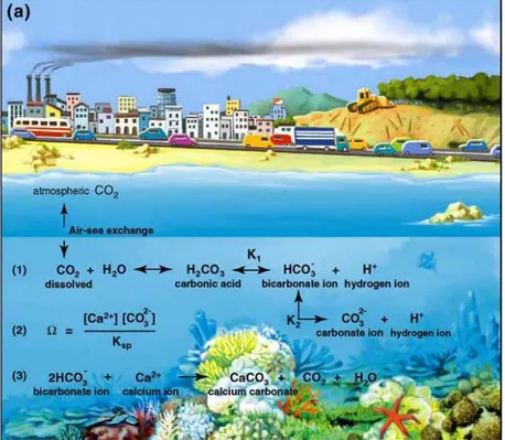
The ocean acidification is a phenomenon caused by the increase of carbon dioxide in the atmosphere. The increase of carbon dioxide in the atmosphere is mostly caused by human activities. In particular 50% of the CO2 in the atmosphere derives from oil extraction, while 30% is caused by deforestation.

There is a correlation between the increase of CO2 in the atmosphere and decrease in pH value in the oceans. In fact at the air-ocean interface there is a continuous exchange of carbon dioxide.

CO2 dissolves in seawater and participates in a series of chemical equilibrium reactions (Figure n.3) which result in increased concentrations of bicarbonate and hydrogen ions (protons) and therefore leads to a decrease in seawater pH (Figure n. 4). This also leads to an increase in the solubility of carbonate ions, with implications for marine organisms that need them as building blocks in the construction of their calcium carbonate skeletons or shells. Experimental studies have demonstrated that this change in seawater chemistry makes calcification more difficult for most of these organisms. Sea organisms can precipitate calcium carbonate in the form of calcite (e.g. coccolithophorids, foraminifera), aragonite (e.g. corals, pteropods), or high-magnesium calcite (e.g. crustose coralline algae). These crystal structures have different degrees of stability and solubility. Calcite is thermodynamically the most stable, followed by aragonite and finally by high-magnesium calcite, which is the least stable (most soluble in decreasing pH). The tendency for a structure to dissolve is strongly influenced by the saturation state of each particular mineral phase, which is related to the concentration of calcium and carbonate ions in the seawater (Pelejero et al. 2010 ).

Figure n.3 Chemical equilibrium reaction of CO2 dissolved in seawater : CO2 reacts with water giving rise to calcium carbonate

which is in acid-base balance with carbonate and carbonate ions which in turn react with calcium ions to produce calcium carbonate.

(Pelejero et al.2010)

Figure n. 4 The increase of carbon dioxide in water increase concentration

of bicarbonate and Hydrogen ion and then reduces pH value of seawater (Pelejero et al.2010)

Impact on marine invertebrates life

The reduction of calcium carbonate available in the water due to it is increased solubility, can reduce the ability of the invertebrate organisms with calcareous skeletons to produce these structures.

However this is only one of the affects caused by ocean acidification. In fact the responses of marine organisms are variable and depend on the type of process affected by acidification (dissolution and calcification rates, the growth rates, development and survival etc.).

There are mane different hypotheses to explain the variations seen in biological responses:

- Organisms that have a calcium carbonate skeleton will be more sensitive to ocean acidification in comparison with organisms without calcium carbonate skeletons;

- Organisms that have more soluble mineral forms of CaCO3 (aragonite) will be more sensitive than organisms with less soluble mineral forms (calcite); - Early states (embryos and larvae) will be more sensitive than adult stages; - mobile organisms with high metabolic rates may be are more able to

compensate for variations in chemistry of calcium carbonate in comparison with sessile organisms with a lower metabolic rates (Kroeker et al. 2010); - Autotrophs with a less efficient or absent carbon-concentrating-mechanisms

(CCMs) will be more responsive than organisms with a efficient CCMs (Rost & Riebesell 2004; Engel et al. 2005; Riebesell et al. 2000).

Calcification may be especially sensitive to variations in carbonate chemistry. The reduction in calcification rates or increase in dissolution rates of CaCO3 have been

measured in tropical corals (Kleypas et al. 1999; Marubini et al. 2003; Hoegh-Guldberg et al. 2007), planktonic organisms (Riebesell et al. 2000; Orr et al. 2005), bivalves (Michaelidis et al. 2005; Gazeau et al. 2007) and echinoderms (Kurihara & Shirayama 2004; Shirayama & Thornton 2005). The sensitivity and variation in carbonate chemistry depends on the calcifying organisms. In particular the sensitivity may be dependent on the mineral form of CaCO3 used by the organism. In fact, different mineral forms have a different solubility and susceptibility, these increase from low magnesium calcite to aragonite and high-magnesium calcite (Morse et al. 2006; Ries et al. 2009).

There is the possibility that some species may be able to change their calcification ratios to control the variation in calcium carbonate concentration, or others are able to control their calcification under differing ph conditions (Gutowska et al. 2008). Moreover some calcareous organisms such as corals and algae are in symbiosis with autotrophic such as algae and for this reason may be this calcareous organisms are able to compensate the ocean acidification through interaction between calcification and photosynthesis. Therefore photosynthesis may be able to reduce the negative effects caused by ocean acidification (Ries et al. 2009).

As regard the different stages; larvae and juveniles are typically more sensitive to environmental condition and can suffer extremely high mortality. Probably because in these stages they use a more soluble mineral form of CaCO3 than when they are adults (Pechenik 1987).

For example some echinoderms larvae (e.g. brittlestars) show a high mortality during larval stages when they are exposed to ocean acidification. However the analysis of the literatures reveals that echinoderms are surprisingly robust to OA and that

important differences in sensitivity to OA are observed between populations and species (Dupont et al. 2010).

Ocean acidification also can disrupt the acid-base status of extracellular body fluid (blood or haemolymph), but some organisms such as fishes, cephalopods and some crustaceans can control extracellular pH through active ion transport (Kroeker et al. 2010).

EFFECTS OF OA ON RESPIRATION AND REGENERATIVE CAPABILITIES OF Amphiura filiformis:

Echinoderms are often playing the role of keystone organisms in the marine ecosystem and they are also present in almost all of the marine ecosystems. They are usually use for toxicology experiments and were extensively used as model to study the effect of the ocean acidification (Dupont et al 2010). Echinoderm skeletons are made of high-magnesium calcite that is particularly susceptible to dissolution when there is a decrease of pH values (Shirayama and Thornton 2005).

The phylum Echinodermata is characterized by 5 classes, including the Ophiuroidea or brittlestars. Ophiuroidea have an exceptional regenerative capabilities.

The brittlestar A. filiformis is one of the dominant macrofaunal species on soft-bottoms in the north-east Atlantic at depths from about 15 m down to 100 m or more (O'Connor et all 1983, Kiinitzer et al.1992). This species is buried in the sediment with its disk at about 4 cm depth (Figure n. 5). One or 2 arms are stretched up above the sediment for feeding. A. filiformis can switch between suspension and deposit feeding depending on current speed and availability of food (Buchanan 1964). During the inactivity moment, the arm tips are kept at the sediment water interface. When the arms are extend in the water column, they are easy prey by visual predators commonly present in the same habitat, e.g. Limanda limanda and Nephrops norvegicus. In order to reduce predation A. filiformis has developed several adaptation (Wilkie, 1978; Bowmer and Keegan, 1983; Herring, 1995; Rosenberg and Selander, 2000; Rosenberg and Lundberg, 2004).

Nevertheless the adaptation is really common find that more than 84% A. filiformis individuals show evidence of regeneration following amputation or more than 80% of arms showing at least one scar (Sköld and Rosenberg, 1996).

Figure n. 5 A.filiformis

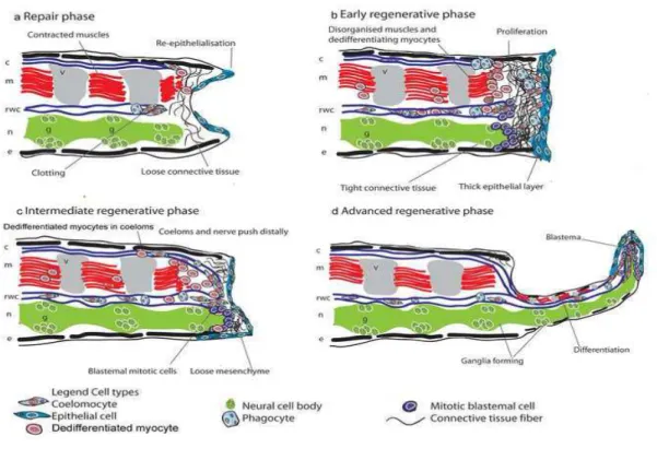
The regeneration process is characterized by different stages. At the beginning it is possible to individuate an epithelium that cover and protect the amputated part. After some days the amputated part is characterized by the presence of a blastema, which is constitute by undifferentiated cells. In the later regenerative phase it is possible recognize two distinct part: a distal part, characterized by undifferentiated cells, and a proximal part with segments fully formed, whit clearly developed ossicles, podia and spines. The anatomic analysis at the microscope (Figure n. 6) of a regenerating arm of A. filiformis, permit to describe the different stages that characterized the regeneration:

- 1 day after the amputation it is evident a thin epithelium that covers the damaged part and the distal injured ends of the main coelomic cavities and canals are already sealed off; coelomocytes (types of leukocytes that constitute the major immune defence system of annelida, mollusca and arthropoda) and phagocytes (white blood cells). It is also possible to individuate in the surface of the stump autotomy the

presence of the muscular remain (aboveral invertebral muscles) belonging to the segment involved in the autotomic process and detached by their distal skeletal insertions.

- 3 days after the amputation, it is evident a small blastema, consisting of a mesenchyme covered by an outer thick apparently pluristratified epithelium. The outgrowth of the main coelomic cavity appears to project into the regenerative blastema and it is associated with a sheath of fibrous mesenchymal matrix. Groups of free cells could frequently be detected inside the coelomic cavity. The aboral muscle of the stump bundles involved in autotomy, acquired a remarkable disorganized pattern, showing a number of dedifferentiating myocytes.

- 4-6 days after the amputation, the blastema is well developed and in this structure is filled by cells, presumptive undifferentiated coelomocytes and the fibrous matrix is poorly developed except in the proximal region. The radial nerve cord grow again, associated with the outgrowth of the previsceral coelom and the radial water canal. At the level of the stump aggregation of coelomocytes, phagocytes and dedifferentiating myocytes are frequently detectable inside the coelomic cavities. Especially In the distal region the muscles show a characteristic disarranged pattern. - 8-12 days after amputation, the proximal portion of the regenerating arm is dominated by the outgrowth of : radial nerve with is ganglionated structure, previsceral coelomic cavities and the radial water canal with new podia. While in the distal portion still present a typical undifferentiated blastema.

- 16-24 days after the amputation, the regenerating arms looking as a miniature arm. The proximal portion show a typical hystological pattern characterized by the prominent presence of the radial nerve cord, differentiated coelomic components and differentiated epineural sinus, vertebral ossicles with associated invertebral ligaments

and muscles, and superficial skeletal arm shields. The distal tip of the regenerate retained the features of an undifferentiated blastema (Biressi et all 2010).

Figure n. 6 Generalized scheme of Ophiuroid arm

Regeneration ( Biresi et al. 2010)

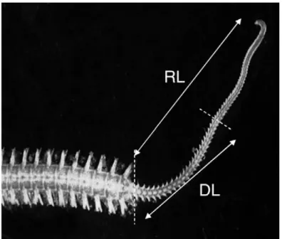
Dupont and Thorndyke (2006) analyzed the difference in the grow capability in the A filiformis. During their experiment they measured for each organism the diameter of the disk, the length of the arm lost (LL) and the regenerated length (RL). The regenerated length (RL) is the whole animal’s arm regenerated, while the differentiated length (DL) is the proximal part with completely formed segments, clearly developed ossicles, podia and spines.

In order to reduce the variability, between the regenerating arms of different organisms, they cut the arms at the same distant from the tip. In this way it was

possible to have a similar regeneration and differentiation rate. The results indicated that the length lost (LL) is a key fact that can explain the variability for regeneration and differentiations rate. Also the analysis evidenced a positive exponential relationship between length lost (LL) and regeneration rate (RR) (Figure n.7). In fact arms cut close to the disc regenerated faster in length than those cut close to the tip, although overall function recovery of the arm are lose (Dupont and Thorndyke 2006).

Figure n. 7 relationship between the length lost (LL) and the regeneration rate (RR).

The range was about 0.5 – 3.5 mm.week-1 ( Dupont and Thorndyke 2006).

Figure n. 8 RL regeneration length and DL differentiation length.

(From Dupont and Thorndyke 2006).

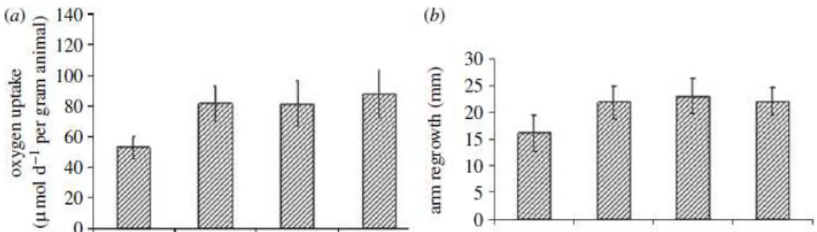
Impact of the ocean acidification on regenerative capability of A. filiformis was previously investigated by Wood et al. (2008). Their experiment was carried out using the ambient temperature and the individuals of A.filiformis were maintained in sediment cores without food and supplied with filtered seawater. Wood et al. (2008) exposed the individuals for 40 days to varying degrees of acidification ( pH 8, pH 7,7, pH 7,3 and pH 6,8), and monitored the regeneration and the respiration. The results show that ocean acidification increase the rate of calcification and metabolism, with a significant increase of the respiration (Figure n. 9). On the other hand, the muscles mass showed a reduction in mass decreasing pH value, and it was hypothesized that brittlestars use the muscles mass as an energy source under stressing conditions (Wood et al. 2008).

Considering these results and also the hypothesis that the species’ thermal window (which is the range of temperature within which it is possible to live for an organisms) will be reduced under low pH condition as suggest by O. Pörtner and P.

Farrell (2008). I tested the impact of short term exposure to low pH on A. filiformis. along the temperature range they experience through the year(6 to 18°C).

The thermal window is individuated between the lower and upper critical temperature. Every organisms have also an optimum of temperature, which correspond to the maximum performance for the organism (Figure n 10). Pörtner and Farrell (2008) supposed that the performance was influenced by the ocean acidification. In fact in their article they hypothesized that the increase of pCO2 was responsible of a reduction of the performance’s curve and then of the thermal window’s range and the optimum of temperature.

MATERIALS AND METHODS:

Figure n.9 results from Wood et al (2008) about respiration and regeneration of Amphiura

filiformis in different pH conditions (Wood et al.2008).

Figure n. 10. temperature effects on aquatic animals. Show the variation of the

MATERIALS AND METHODS

Experimental set-up

A. filiformis is an Echinoderm which lives in the sediment. The organisms were collected at 25 – 40 m depth, using a Petersen mud grab, near Kristineberg Marine Station, Sweden. Immediately after, the organisms were sampled form the sediment cores by gentle rising to avoid breaking arms and transferred to the experiment set-up in order to acclimate the organisms to the right temperature. The period of acclimation for the temperature was of 2 weeks, during which the temperature was changed of 1 degree a day. pH value was manipulated in the treatment using a computerised control system called AquaMedic, this instrument regulated the pH value by the addition of pure CO2 directly into the water to obtain a reduction of 0.04

pH units. The organisms were maintained in plastic tanks without sediment and with a continuous seawater flow, which allowed a continuous supply of food.

The experiment was carried out for a period of 4 weeks. The organisms were exposed to six different temperatures: 6°C, 10°C, 12 °C, 14°C, 16°C and 18°C and for each temperature two different pH values: one control pH 8,1 and one treatment pH 7,7, every combination was replicated 2 times replicates with 2 pseudo-replicates containing 50 non-regenerating A. filiformis each replicates. The amputation of the organisms has been induced on individuals that showed no evidence of recent regeneration. The organisms were anaesthetized using a solution of artificial water and 3,5 % w/w MgCl2. The arms were amputated using a scalpel blade across a natural inter-vertebral autotomy plane. The arms were cut a constant distances from

the tip to reduce the variability of the regeneration, how suggested by Dupont and Thorndyke (2006) in their article.

Effect of OA on respiration of Amphiura filiformis

I measured the respiration of 10 amputated organisms (chose random) for each combination of temperature and pH and for a period of four weeks.

The instrument used to measure the percentage of Oxygen breathed by the organisms, it was the 4-OXY-Micro. The machine was connected to 4 probes, which measured the percentage of oxygen and to a computer, which showed the values measured with the instrument. Before starting the measurements the probes were calibrated as suggested the manufactory manual (PreSens 4-OXY Micro, Germany). I filtered 2 L of seawater with a filter of 0,45 µm and we bubbled oxygen into this water for 24 hours in order to saturate the water with the oxygen. The bottle with the 2 l of water was placed in a bath to obtain the right temperature. Subsequently in the bath I put two bottles of 500 ml that I filled with the saturated filtered seawater. In one we bubbled oxygen and pure CO2 in order to obtain the right pH treatment that was cheeked through a pH meter. While in the control bottle we bubbled only oxygen. I used 14 vials for the control measurements and 14 for the treatment, we filled the vials with the control and treatment saturated FSW, respectively and in each vials I put one individual of A. filiformis, accepted in the first 4 vials of control where there was only saturated FSW and in the last 4 vials of treatment. The instrument permitted to measure the percentage of oxygen for 4 vials at time, for this reason in total we have done 7 battery of measure with 4 vials each. Once I finished the first battery of measurement, it was necessary to wait for a certain period of time

(respiration time) before starting with the second measurement. During this period of time the organisms consumed some oxygen breathing. The percentage of oxygen consumed depends on the temperature. The respiration rate degrees with decreasing temperature; in fact the organisms exposed to low temperature as 6°C breath slower than the organisms exposed at 18°C. The respiration time for each temperature was:

- for 14°C and 16°C: 2 hours; - for 10°C and 12 °C: 4 hours; - for 6°C: 6 hours;

- for 18°C: 1 hour and 30 minutes.

After this period of time it was possible to start with the second measurements, which permitted to individuate if there were differences between treatment and control. After the second measurements I weighed the organisms putting they a solution of artificial water and 3,5 % w/w MgCl2 at the same temperature of the experiment, in order to reduce the stress for the organism. I also measured at the microscope for each organisms the length of the regenerating arm and the diameter of the disc. The collected data of respiration and weight have permitted to calculate the respiration rate, which was measured using the ANOVA (simple ANOVA 1 replicate used for each combination of temperature) and was expressed in µmol O2 ind -1 h-1.

Effect of OA on regeneration of Amphiura filiformis

For a period of 4 weeks, after that the amputation regenerate length and the disk diameter, were measured by taking a pictures of the regenerating arms of 10 organisms in each pseudo-replicates for each combination of temperature and pH. I

took some pictures of the organisms using a graduated ocular in binocular microscope (0,1 mm accuracy), and later I calculate the regeneration length of the organisms. The regeneration length (RR, in mm week -1) was calculated as the slope of the significant simple linear regeneration between the regenerated length (RL in mm) and time in weeks how indicated in the article of Dupont and and Thorndyke (2006).While the difference in the regeneration rate between pH for each temperature was tested using ANCOVA and using time as the co-variable.

RESULTS

Regeneration

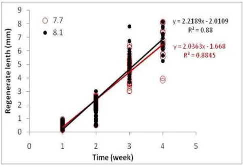
The regeneration length for each combination of temperature and pH have been calculated in order to evidence the possible differences between the control and the treatment. In order to calculate the regeneration rate for each combination of temperature and pH the regression coefficient between regeneration length and time was calculated. In the Figure n.11 for the temperature 14°C were plotted in order to calculate the regeneration rate, the data length collected in 4 weeks in both control and treatment and the linear regression with the respective straight line equation were calculate. Table n 1 show for each combination of temperature and pH the coefficients a and b of the straight line equation (size = a *time + b), the coefficient of determination (R2) and the test F. The coefficient of determination (R2) indicated how well the regression line approximates the real data points, in particularly in the experiment the values of R2 indicate that there is a good approximations of the data plot because the R2 values are near to the value 1, except for the control pH of the temperature 6°C. Table n 2 shows the regeneration rate for each temperature and in particular it is evident that there are not a significant differences in the regeneration rate between control and low pH for each temperature (p<0,005), except for the regeneration rate value of temperature 6°C, which was significantly slower at low pH. Figure n. 12 shows the curves of regeneration rate for control and treatment calculated for all the temperatures tested and the significant value (p < 0,005).

Figure n.11. for the temperature 14°C linear regression of the

control and the treatment for a experimental period of 4 weeks.

pH Temp. a± standard error b± standard error F p R2 7,7 6 0,069±0,005 - 0,076±0,014 184,50 <0,001 0,574 8,1 6 0,075±0,008 -0,068±0,022 81,11 <0,001 0,335 7,7 10 0,922±0,03 -1,00±0,06 968,95 <0,001 0,861 8,1 10 0,819±0,03 -0,829±0,082 723,64 <0,001 0,828 7,7 12 1,348±0,049 -1,350±0,121 765,50 <0,001 0,850 8,1 12 1,403±0,06 -1,36±0,150 549,73 <0,001 0,805 7,7 14 2,036±0,065 -1,668±0,161 965,37 <0,001 0,884 8,1 14 2,219±0,07 -2,012±0,172 1005,08 <0,001 0,880 7,7 16 2,501±0,092 -1,698±0,211 743,51 <0,001 0,858 8,1 16 2,494±0,126 -1,62±0,304 391,19 <0,001 0,748 7,7 18 2,072±0,121 -0,97±0,28 294,31 <0,001 0,710 8,1 18 2,281±0,106 -1,160±0,240 462,49 <0,001 0,795

Table 1. linear regression: show for each combination of temperature and ph:

Ancova Time pH Temp. F p F p F P 6 101,17 <0,001 200,59 <0,001 4,03 0,0455 10 830,11 <0,001 1656,91 <0,001 2,95 0,0867 12 6,36,12 <0,001 1269,42 <0,001 2,18 0,1409 14 972,11 <0,001 1943,68 <0,001 0,44 0,5099 16 494,73 <0,001 985,1 <0,001 0,18 0,6731 18 365,65 <0,001 726,46 <0,001 2,17 0,1423

0

0,5

1

1,5

2

2,5

3

0

5

10

15

20

Temperature (C)

R

e

g

e

n

e

ra

ti

o

n

r

a

te

(

m

m

.w

-1

)

_8,1

7,7

Poli. (8,1)

Poli. (7,7)

*

Table 2. ANCOVA analysis of co-variance show the

p-values and the F p-values

Figure n. 12. Regeneration Rate: show the regeneration rate

Respiration

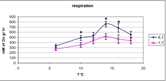
Table n. 3 shows the results for respiration rate calculated using the sample ANOVA. In particular is evident that the respiration rate was significantly reduced under low pH condition for the temperatures:10°C, 14°C and 16°C. While no significant differences were observed for the other temperatures. Figure n. 13 shows the curves of respiration, both controls and treatments.

respiration 0 100 200 300 400 500 600 700 800 900 0 5 10 15 20 T °C m M o f O x g r h r 8,1 7,7

*

*

_*

Table 3. analysis of variance. significant differences (p<0,001) in the

IMPACT OF OCEAN ACIDIFICATION ON Ostrea edulis LARVAE STAGES:

As regard the impact of the ocean acidification on bivalves larvae many studies have been carried out to verify whether or not ocean acidification has effects on larvae development (morphology) and larvae settlement (percentage of survival). Larvae development of several calcifiers is affected by elevations of seawater pCO2 (Kurihara 2008). The experiment of Kuihara (2008) has been demonstrated that larvae of Pacific oyster Crassostrea gigas and Mytilus galloprovincialis were strongly affected by high pCO2 conditions in his experiment. oyster eggs reared under 1000 µatm pCO2 (pH 7,8), showed malformations such as convex hinges, a characteristic that is usually used to identify abnormal development of veliger larvae. While when oysters eggs were reared under 2000 µatm pCO2 (pH 7,4) more than 70% of the larvae were completely non-shelled, or only partially shelled, and only 4% of CO2 treated embryos developed into normal ‘D-shaped’ veliger larvae by 48 h after fertilization, whereas in the controls about the 70% of embryos developed into the normal veliger stage. In comparison with larvae of oysters the larvae of the mussel, M. galloprovincialis were completely shelled in these treatments, although the size was about 20% smaller than that of larvae from the control and also showed morphological abnormalities such as convex hinges, protrusion of mantle and malformed shells. These results suggest that high pCO2 affected larva skeletons and the shape of the shells.

As regard the effect on larval settlement of juveniles, Mercenaria mercenaria the results of Kurihara (2008) showed that the shell dissolution rates and mortality were highly influenced by CaCO3-undersaturated conditions. It is also clear that the affects

of the ocean acidification are different between larval and adult stages; for example in oyster larvae, calcification in the treatment with 2000 µatm pCO2 (pH 7,4) is 50% less in comparison with the calcification of oyster adults in the same pH. This probably is due to the difference between the shells of adults and shells of larvae. In fact adults’ shells are composed of calcite, while in the larval shells the major form of CaCO3 is Aragonite. Aragonite is more soluble in comparison with calcite and for this reason larval stages are more affected by the variation in pH values (Kurihara 2008).

In the experiments of Talmage and Gobler (2009) the effect of OA on scallops Argopecten irradians and Eastern oysters Crassostrea virginica has been studies. A.irradians larvae were extremely sensitive to higher CO2 concentrations (≈152 Pa CO2) only 3 % ± 1 % and 2 % ± 0.5 % of A.irrafians larvae survived to metamorphosis at ≈ 62-Pa and 170-Pa CO2 levels, while 52 % survived in the ambient treatment (≈39 Pa CO2). Whit regard to the effects of high CO2 levels on development rates of A. irradians larvae: after 16 days only the 54 % and 76 % of scallop larvae had metamorphosed to the juvenile stage at 170 and 62 Pa CO2, whereas under control conditions (≈36 Pa CO2) the percentage of survivors was 100 %. At day 19, the lengths of A. irradians larvae grown under high CO2 were half the size of individuals grown under ambient CO2 conditions.

C. virginica larvae responded differently to the increase of CO2 in the seawater; here the rate of oyster larvae metamorphosis was significantly delayed by exposure to high values of CO2. In fact after two weeks, one third of the oyster larvae exposed to current CO2 levels had fully metamorphosed, while only 6 % ± 2 % and 3 % ± 1 % had done so at ≈ 66 and 152 Pa CO2 respectively. After 3 weeks metamorphosis in current condition of CO2 levels, had taken place in 89%, while at ≈ 66 and 152 Pa

CO2, the percentage of larvae to metamorphosis was 69 % ± 12 % and 58 % ± 12 % respectively. The effect of high CO2 levels (64 and 150 Pa) on lengths on C. virginica larvae, was that their length was significantly smaller than those grown at ambient CO2. However, there were no differences in survivorship between exposure to 35 and 66 Pa CO2 (61 % ± 16%), while the larvae exposed to the highest level of CO2 (≈152 Pa CO2) showed a significant reduction in survival percentage at 35 % ± 13 % (Talmage and Gobler 2009).

Considering the negative effect of OA on larvae stages and the economic importance of O. edulis I tested if a reduction in pH values of 0,4 units affects the growth, morphology and the survival of O. edulis larvae.

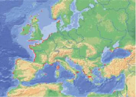
The European flat oyster, Ostrea edulis, is a native specie in Europe, but nowadays it is possible to find it in various other parts of the globe. Initially present in Norway, it has migrated to Morocco, North-East Atlantic and the Mediterranean. Natural populations are also observed in eastern North America, from Maine to Rhode Island, following intentional introductions in the 1940s and 1950s. The specie was also introduced in Canada for aquaculture purpose 30 years ago and some populations naturalised in Nova Scotia, New Brunswick and British Columbia. These stocks were imported from naturalised populations in Maine whose ancestors originated in the Netherlands(Figure n.14).

O. edulis is a mollusc typical of the intertidal zone and it is characterized by two valves: the lower (left) valve is convex and upper (right) valve is flat. It lives on firm ground in shallow coastal waters down to a depth of 20 m.

O. edulis is a Protandrous hermaphrodite, and in fact during the spawning season changes sex twice:

- then there is a transition from male to female; - then again transition from female to male.

Fertilization is in the mantle cavity and the number of eggs produced can reach a million and a half. After 8-10 days of incubation in the mantle cavity the larvae are released and they have a diameter of around 160 µm. The dispersive pelagic phase last approximately 2-4 weeks (depending on the temperature) after this period the larvae become adults (Lapègue et al. 2006).

The pelagic phase is characterized by different stages (Figure n.15):

- first stage of development immediately after the release from the adult is to veliger or D-shell or the straight hinge stage (147±5.0 x 126±7.2 µm): larvae remain at this stage for about 5 days during which they are translucent and move via the strong current produced by the ciliated velum;

- - second stage is to veliconcha or early Umbo (210±8.99 x 185±12.11 µm): after 5 days the larvae undergo a morphological change as the boss becomes slightly oval and the shell itself takes on an oval shape. The ability of the larva to move is reduced compared to the veliger stage; - third stage is Umbo: in this phase is easily distinguishable the “Umbo”(this is a thickening of the shell; 239±30.32 x 208±29.26 µm) and the ability to move is further reduced. This stage is usually reached about on the fourteenth day after release from the adult.

The last stage is to pediveliger: (average 254±33.37 x 233±33.83 µm) and this metamorphosis takes place around the seventeenth day. During this phase the foot and the eye spots become visible.

The larvae tend to stay deeper in the water column and move along the substrate with the help of the foot (Sefa Acarli and Aynur Lok 2009).

Figure n.14 Distribution of Ostrae edulis (Lapègue et al. 2006).

MATERIALS AND METHODS

In the first part of the experiment, in order to obtain the pH values in the treatment I used an air/CO2 mixing system. With this system it was possible to mix air (380 ppm of CO2) from the atmosphere and Carbon dioxide using a bottle of 590 ppm CO2. In this way it was possible to introduce a mixture of carbon dioxide and air with 970 ppm of CO2 in the filtered deep seawater and to obtain the value of pH predicted for the end of the 21st century. With the air/CO2 mixing system it was also possible to reproduce the natural fluctuation of the carbon dioxide in the seawater. The fluctuation of the carbon dioxide in the seawater depends on photosynthesis during the day and respiration during the night (Figure n.16). After 2 months of work (from April until the end of May) the results given by this machine were always the same; in fact there were never any difference in pH values between the bottle connected with air/CO2 system and the bottle with just air (Figure n17).

Since the gas mixing system failed, in the second phase of the experiment the system was changed and pure CO2 & Aqua-Medic systems were used to obtain treatment pH values. Moreover plastic bags with about 5 L of filtered deep seawater were used. Of those bags: 4 bags were for the treatment and were connected with Aqua-Medic systems and 4 for the control (≈ 8,1 pH) connected only with air to assure the circulation inside the bags. The Aqua-Medic system was connected with a bottle of pure Carbon dioxide and air from the atmosphere, the pH value in the bags was checked using a pH meter (one for each treatment bags). When the pH values changed, the valve delivering pure CO2 was opened by the Aqua-Medic system to stabilize the pH treatment value. This value was established connecting for one day a sample of filtered deep seawater with a bottle of carbon dioxide (970 ppm of CO2). In this way the pH value for the treatment was 7,78. The O. edulis larvae used for the first experiments were taken from Anders’s adult oysters culture at Tjärnö field station, whereas for the second and third experiments larvae from the oyster hatchery (Koster Island) were used. In each bag there were about 75 000 of larvae but in the

pH bottles CO2 Box-air

7,8 7,9 8 8,1 8,2 8,3 21/05/2010 17.25 22/05/210 7.30 22/05/210 11.00 22/05/210 15.40 22/05/210 19.30 23/05/2010 9.00 23/05/2010 13.00 23/05/2010 17.00 23/05/2010 21.00 24/05/2010 8.25 date ph Bottle air/CO2 Bottle air

Figure n.17 plot of the pH values in a bottle with air/co2 system and in a bottle with only

3th experiment they were only about 40 000 larvae because the production of larvae in hatchery was reduced.

The water in each bag was changed every 3rd day, and 3 samples of water were taken from each bag to count the survivors and to prepare slides in order to measure the length and width of 75 organisms.

Figure n 18 show the means of the length measured for 100 organisms. In particularly in the graph are plotted the means for the first 5 measurements, for the first 10, 15 and so on, for a total of 100 organisms. In this way it was possible determined how many larvae we needed to measure to get an accurate mean for the length and width. The graph show that there is a stabilization of the curve at the value 75th. For this reason in our experiments we measured the length and width of 75 organisms. length 176 178 180 182 184 186 mea n 5 mea n 15 mea n 25 mea n 35 mea n 45 mea n 55 mea n 65 mea n 75 mea n 85 mea n 95 m ic ro m e te rs length

Effects of OA on the percentage of survivors

Every third day I changed the water in the bags and I took three sample of a certain volume of seawater with a pipette for each control and treatment. I putted the seawater with the oysters larvae in three small Petri dish and I counted at the stereoscope, the number of the organisms that were alive. Later I anesthetized the organisms putting some drops of MgCl2 solution in the seawater and I counted the total number. I have done the same procedure for the 3 experiment and I calculated for each experiment the percentage of survivors.

Effects of OA on the growth and morphology

From the same sample takes to count the number of organisms alive I took a sample with the pipette and I prepared a slide for each control and treatment. I analyzed at the microscope the morphology of oysters larvae and I measured the length and the width for 75 organisms excepted for the first experiment, where I took the measurements only for 20 organisms.

During the analysis at the microscope I also took the picture for each slide of each experiment.

To verify if there were differences in the percentage of survivors between control and treatment I analyzed the data using the repeating measuring ANOVA. As regard the analysis of the survivors data the experimental design was not balances, in fact in the first experiment for the factor Time the level are 4 while in the experiments n.2 and n.3 the Time has 3 level because the organisms died faster than in the experiment n.1.

The experimental design for the survivor data in the experiment n.1 was: Factor 1: treatment 2 levels is orthogonal and is fixed;

Factor 2: is replicates 4 levels is nested within treat and is random; Factor 3: is time 4 levels is orthogonal and is random.

While for the experiment 2 and 3 was:

Factor 1: treatment 2 levels is orthogonal and is fixed;

Factor 2: is replicates 4 levels is nested within treat and is random; Factor 3: is time 3 levels is orthogonal and is random

As regard the analysis of the data about the measurements of the length. The experimental design was:

Factor 1: treatment 2 levels is orthogonal and is fixed;

Factor 2: is replicates 4 levels is nested within treat and is random; Factor 3: is time 3 levels is orthogonal and is random

In the repeating measuring ANOVA are important the Test of Within Subjects effects and Tests of Between-Subjects Effects; In a within-subjects design, each variable is tested under each condition. The alternative to a within-subjects design is a between-subjects design. In this case, each variable is tested under one condition only.

RESULTS

Percentage of survivors

The Table n. 4, 5 and 6 show the means values (± 1 Standard Deviation) of the survival in the control and treatments during the experimental period. Data and error from each experiment have been plotted in separate graphs. Similar trends have been observed in both control and treatment of each experiment, as show in the curves in Figure n. 18, 19 and 20. In particular in the graph n. 5 referring to the experiment run on the 7 July 2010 differences in the curves between control and treatment are evident. The t-test made on these data shows that there is not a significant difference between control and treatment (Table n 7).

Treatment Date Mean Surv SD Surv control 11/06/2010 100 Control 14/06/2010 97,2111754 0,958878 Control 17/06/2010 96,931767 0,121417 Control 20/06/2010 32,8687861 9,303957 Control 23/06/2010 4,77871565 0,963322 Treat 11/06/2010 100 Treat 14/06/2010 90,2384996 1,820209 Treat 17/06/2010 96,8476425 0,511429 Treat 20/06/2010 26,4530245 5,985484 Treat 23/06/2010 0,55671056 6,472971

Table n.4 experiment n.1mean of survivors and standard deviation

Treatment Date mean surv SD surv Control 07/01/2010 100 Control 07/04/2010 96,20218052 1,022411278 Control 07/07/2010 61,03939949 5,159934265 Control 07/10/2010 17,89330494 1,022411278 Treat 07/01/2010 100 Treat 07/04/2010 95,25137727 1,022411278 Treat 07/07/2010 76,47256334 6,931189563 Treat 07/10/2010 19,74811248 2,900007229

Table n.5 experiment n. 2mean of survivors and standard deviation

for the control and treatment

Treatment date mean surv SD surv Control 16/08/2010 100 Control 19/08/2010 97,05938037 1,058620097 Control 22/08/2010 56,10480399 6,867863633 Control 25/08/2010 11,35150324 3,912368945 Treat 16/08/2010 100 Treat 19/08/2010 96,18888362 1,601164424 Treat 22/08/2010 59,03627248 7,477946359 Treat 25/08/2010 10,17990525 2,018652225

Table n.6 experiment n.3 mean of survivors and standard deviation

ex. n1 mean surv

0

20

40

60

80

100

120

Figure n. 18 means of survivors for the experiment n1

ex. n2 mean surv

0 20 40 60 80 100 120 14/10/2009 22/01/2010 02/05/2010 10/08/2010 18/11/2010 date s u rv iv o rs control treatment

ex. n3 mean surv 0 20 40 60 80 100 120 14/08/201 0 16/08/201 0 18/08/201 0 20/08/201 0 22/08/201 0 24/08/201 0 26/08/201 0 date s u rv iv o rs Control Treatment

Figure n. 20 means of survivors for the experiment n3

t test comparing survivals of treatments vs controls (n=4)

P value (2-tailed, unpaired) = 0,426351

Table n.7 t-test

In order to individuate differences in the survival of O.edulis between controls and treatments, repeated measuring ANOVA was used to analyse the survival Independent measurement from the same replicate were collected at each time.

Tables n.8 shows the results of the test of Within Subjects effects and in particular the Type III Sum of Squares, which is used when the design is unbalanced. In fact in the first experiment survivors were counted 4 times while in the others two experiments larvae died faster and measurement were done only 3 times. Sphericity was tested using the ”Greenhouse-Geisser” test. Sphericity requires that the variances for each set of difference scores are equal. To assume the occurrence of sphericity

the results of Greenhouse-Geisser test would be positive (P > 0,05). In the experiments, values of Greenhouse-Geisser test were about 0,05 except for the interaction between time* treat*exp. In the table it is possible to note that the factor time is significant and also interaction between times*exp were significant (p < 0,001).

The results of the test in the effects between subject are showed in table 9. This table displays the labels of all the values for all the levels of the between-subjects factors. The test shows that p differences between experiments are significant

Test of Within-subjects Effects

Type III Sum of Squares df mean square F Sig measurements_times Greenhouse-Geisser 10,82 2 5,445 395,264 000 measurements_times*treat Greenhouse-Geisser 0,067 2 0,034 2,454 100 measurements_times*exp Greenhouse-Geisser 0,788 4 0,197 14,391 000 measurements_times* treat*exp Greenhouse-Geisser 0,023 4 0,006 0,42 0,793 Error (measurements_times) Greenhouse-Geisser 0,493 36 0,014

Tests of Between-Subjects Effects

Source

Type III Sum of

Squares Df Mean Square F Sig.

Intercept 66.530 1 66.530 2776.477 .000

treat .006 1 .006 .252 .622

exp .941 2 .471 19.644 .000

treat * exp .058 2 .029 1.207 .322

Error .431 18 .024

Table n.9 repeating measuring ANOVA survivors data, Test of Between-Subject Effects

Growth and morphology

In order to test morphological differences of the larvae of O.edulis between controls and treatments, for each experiment larval length were plotted against larval width and the linear regression was calculated. In particular for the experiment n.1 the length and the width for only 20 larvae were measured, and the Figure n 21 show that this sample size was not enough to analyse the relationship between the width and the length with the linear regression. Moreover the value of the coefficient of determination (R2) is low, showing that there is not a good approximations of the data plot. The others two graphs (Figure n. 22 and 23) show that the linear regressions between control and the treatment are almost overlapping. This can be interpreted as an absence of alteration between length and width since the larvae grow in length and width at the same time. Also the analysis at the microscope of all the larvae sampled, both in controls and treatments slides, did not show any

deformation in any of experiments, both in controls and the treatments (Figure n.24 and Figure n. 25).

To test differences in the growth between control and treatment, all the data about the length measurements collected during the three experiments. In particular in figure n. 26, 27 and 28 data on length were plotted to calculated the growth rate in terms of linear relationship between length and time respectively for the experiment 1, 2 and 3. In the figure n. 27 and 28it is evident that the linear regression between length and time of the larvae, measured in the control and in the treatment sites, are almost overlapping.

While in Figure n. 29 the data of the length measurements during the three experiments were plotted in order to individuate the general trends of the data, with the linear regression calculated for all the data. These data were analysed using ANCOVA. The analysis of co-variance is showed in Table n.10, which is a summary of the p values for the "treatment" effects. The colour red evidences the significant effects. There are no differences in the experiment 1, some significant differences in experiment 2 and 3 (most of the time showing a higher growth rate).

y = 0,6667x + 43,333 R2 = 0,2424 y = 0,7385x + 35,385 R2 = 0,8565 150 170 190 210 230 180 200 220 240 le ngth w id th treat.n2 20-06-10 control n2 20-06-10 Lineare (treat.n2 20-06-10) Lineare (control n2 20-06-10)

y = 0,7951x + 19,327 R2 = 0,8048 y = 0,6739x + 44,515 R2 = 0,8408 140 160 180 200 220 150 170 190 210 230 250 270 length w id th bag treat n2 10/07/10 bag control n2 10/07/10 Lineare (bag treat n2 10/07/10 )

Lineare (bag control n2 10/07/10 )

Figure n. 22 experiment n.2 length against width (data collected in the day 10-07-10)

y = 0,7216x + 38,903 R2 = 0,7274 y = 0,7393x + 34,846 R2 = 0,6406 150 170 190 210 230 250 270 290 180 200 220 240 260 280 300 320 length w id th treatment control Lineare (control) Lineare (treatment)

experiment 1 y = 1,3838x + 185,14 R2 = 0,1945 y = 1,9688x + 182,35 R2 = 0,1672 0 50 100 150 200 250 300 3 6 9 Time (d) L e n g th ( mm ) cont treat Lineare (cont) Lineare (treat)

Figure n. 25 picture of the slide for the treat.Exp.n1

(day4-07-10)

Figure n. 24 picture of the slide for the control Exp. n.1

(day4-07-10)

experiment 2

Figure n.27 linear relationship between length and

time respectively for all of the length data of the experiment 2

experiment 3

Figure n. 28 linear relationship between length and

time respectively for all of the length data of the experiment 3

y = 1,0285x + 0,8204 R2 = 0,5372 0 1 2 3 4 5 6 7 0 1 2 3 4 5 1 2 3 TOT Lineare (TOT)

Figure n. 29 trends of all the data for the three experiments.

experiment 1 2 3 REPLICATE 1 0,341 0,7966 0,0001 2 0,1173 0,449 0,9712 3 0,1729 0,0279 0,0041 4 0,8623 0,0005 0,0001 ALL REPLICATES 0,497 0,0306 0,00001

CONCLUSIONS

Effects of OA on regeneration and respiration in Amphiura filiformis

The results of the laboratory experiments that have been carried out to investigate the potential threats deriving to marine fauna deriving form lower pH values of marine waters shows that an exposure to decreased pH (7,7 vs 8,1 in the control) for four weeks does not have a significant impact on the regeneration rate of A. filiformis across a range of temperatures, with the exception of a slightly lower regeneration rate decrease at the lowest temperature (6°C). This result is contrasting with the result published by Wood et al (2008). In fact in their experiment they found an increase of the regeneration rate in regenerating A. filiforms exposed to a low pH (7,7 vs 8,0 in the control) for 40 days.

The respiration rate of the individuals exposed to lower pH is lower than the respiration rate of the individuals in control water for 3 of the 6 temperatures that have been tested (10,14 and 16 degrees Celsius) while no significant differences were observed for other temperatures (6,12 and 18 degrees Celsius). This is also contrasting with the results of Wood et al (2008) that have shown a significant increase of the respiration rate when individuals ere exposed to similar pH changes. The results of the experiments of this thesis on respiration rate and regeneration rate are in contrast with the results obtained by Wood et al (2008).

The differences results maybe are related to differences in the experimental conditions. In my experimenst the organisms were supplied with a continuous seawater flow, which also allowed a continuous supply of food, while Wood et al did not feed A. filiformis organisms during the experiment, which may have caused addition starvation stress to A. filiformis. In fact during regeneration more energy is

request to regenerate all the segments and if A. filiformis have less energy available they could try to conserve the few energy stored and for this reason reduce the regeneration. As regard the temperature Wood at al (2008) used only one temperature to test the effect of Ocean Acidification, while in the present study different temperatures have been used. Moreover to reduce the variability, between the regenerating arms of different organisms, in this study the arms were cut at the same distance from the tip, while Wood at al (2008) did not standardized the cut and we know from the experiment by Dupont and Thorndyke (2006) that this may cause a high variability of the regeneration and could generate problems during the analysis of the results.

The laboratory experiments show also that ocean acidification may cause a decrease of the respiration rate for the temperatures 10,14 and 16 degrees Celsius. Reduction of the respiration rate may be is caused by a phenomenon called metabolic depression. In fact the organisms exposed to a stressful conditions may save energies by reducing their activities and in our case A. filiformis chose to reduce the respiration in order to have enough energy to use for the regeneration. At the temperature of 6°C the metabolism is reduced, in fact the data show a lower respiration and regeneration reduced in comparison with the values of respiration and regeneration in the higher temperature. Probably for this reason it is more difficult to individuate a difference between control and treatment. A. filiformis plays the role of key species in many seafloor communities (Wood et al 2008), for example this species is responsible for up to 80% of all bioturbation in the sediment (Vopel et al 2003) and if there is a decrease in the number of the specimens present in the sediment this could cause important changes in the bottom bui-geo-chemical process. Considering the worst scenario predicted for the 2100 about the reduction of

the pH values of 0,4 units. It is possible hypothesize that some species can modulate their biological processes in response to the ocean acidification, and this is exactly what is emerging from this study for the regeneration in A. filiformis. The significant effect of the ocean acidification on the respiration, indicated that the metabolisms of A.philiformis could be affected by the variation of pH values and suggest to continue the researches in this field in order to establish criticality of the variation in the metabolism and if it can involve in a reduction of the population in the future scenarios.

Effects of OA on Ostrea edulis stages larvae

The analysis of the survival data shows that OA did not affect the survivor capacity of O. edulis larvae, but there is a significant effect of the time. In fact the number of the larvae that died in both controls and in the treatments was increasing in time. Furthermore it is also significant the interaction between time and experiment and there is a decrease of larvae that survive in the three experiments, compared to the time factor.

As regard the morphology of the larvae all the specimens that have been analysed at the microscope did not show differences in the morphology between control and treatment. The larval development at low pH is normal and follows the development of veliger larvae describe by Thomas R. Waller (1981). The linear regression between length and width of the larvae shows that there are not changes or alteration caused by sea water acidification.

These result about the effect of OA on O. edulis larvae stages are in contrast with the results of Kurihara (2008) about the effects of OA on Mytilus. galloprovincialis, Mercenaria mercenaria and Crassostrea gigas. Kurihara (2008) found that the larvae

shell dissolution rates and the percentage of survivors was highly influenced by the concentration of CaCO3 (Kurihara 2008). Response of O. edulis are also in contrast with the results on A. irradians obtained by Talmage and Gobler (2009).

The analysis of the larval lengths measured during the 3 experiment shows that there are some differences in the length growth between control and treatment in the in the experiment 1, some significant differences in experiment 2 and 3 and that most of the time growth is faster it is impossible to know if the growth rate is higher at low pH, or if the smaller larvae have a higher mortality in that treatment (in which case alteration of the growth rate would be an experimental artefact). In fact in general, the growth rate that have been found in the experiment seems to be very small for the species. This is may be due to the bad quality of the larvae, for the experiments n. 2 and experiment n. 3 the larvae were provided by the hatchery, but unfortunately in the hatchery adult oysters, (probably stressed) did not release or released larvae which appeared to be of poor quality, and the released larvae were also few in number, in fact in the third experiment only 40000 larvae have been used for each bags, while for the others two the number of larvae was 75000.

In conclusion OA is a relative new science and it is believed to be a major threat for near-future marine ecosystems, and that the most sensitive organisms will be calcifying organisms and the free-living larval stages produced by most benthic marine species. In order to verify the real effects of OA on marine ecosystem in these last years the scientific community has increase the number of studies about these field and the experiments were mainly focused on the effects of OA on a broad range of marine species, processes and systems. Many of these are investigating the sensitive early life-history stages that several major reviews have highlighted as