POLITECNICO DI MILANO
School of Industrial and Information Engineering
Master of Science in Energy Engineering
1D THERMO-FLUID DYNAMIC SIMULATION
OF A TURBOCHARGED HEAVY DUTY CI
ENGINE: PERFORMANCES AND EMISSIONS
Supervisor: Prof. Ing. Angelo Onorati
Tutor: Ing. Tarcisio Cerri
Master Thesis of:
Andrea Orsenigo, 836352
Ringraziamenti
Il primo ringraziamento desidero rivolgerlo al Professor Onorati e all’Ingegnere Cerri. Non è un grazie “accademico”, è un messaggio di gratitudine sincera, ma anche di stima per il vostro stile. Siete stati un esempio che cercherò di portare con me nel mondo del lavoro.
Grazie a mamma e papà per aver investito tanto su di me: spero che diventerò l’uomo che sperate. Scusate per i momenti di tensione in cui mi rendevo conto di essere intrattabile. Grazie a nonna e agli altri nonni in cielo, questo traguardo è anche per voi. Statemi sempre vicino e in particolare aiutate mamma e papà nel loro prossimo ruolo di nonni. Grazie a Paolo ed Elisa che ci regaleranno la gioia più grande, almeno per me che non ho mai avuto fratelli/cugini più piccoli. Samuele, ti voglio già tanto bene!
Grazie a voi Amici. Grazie a te, perché condividiamo il nome e abbiamo condiviso molti anni della nostra vita, da compagni di squadra prima, da compagni allenatori poi. Grazie a te, perché anche se entrambi parliamo poco, a noi non servono le parole per capirci. Grazie a te, perché il 9 luglio è sempre più vicino e vivremo un momento fantastico. Grazie a te, perché nel dubbio “ferie”. Grazie a te, perché il pallore è nobiliare, ma che ne sanno gli abbronzati. Grazie a te, perché la vista è importante, ma il buon cibo molto di più. Grazie a te, perché in sei anni e mezzo di Politecnico un tocco di classicismo è un bene prezioso. Grazie a te, perché non pagare mai il cinema (e non solo) è un’arte da imparare. Grazie a voi, perché anche se avete tre anni meno di me, il vostro modo di stare insieme è di esempio per molti. Grazie a te, perché “quando vuoi andare a sciare, ci sono”. Grazie a te, per ogni singolo secondo di vocale (e non solo) degli ultimi 4 anni. Grazie a te, perché la nostra amicizia “I Want It That Way”. Grazie a te, perché anche se ora sei a Bruzzangeles e chissà dove finirai, i momenti insieme non mancheranno. Grazie a te, perché più di tutti mi hai indicato la Via, quando ancora ero un cucciolo di uomo.
Grazie a voi, ragazzi, allenatori e dirigenti perché senza le ore sul campo e in riunione sarei una persona diversa.
Grazie a voi, compagni di liceo, perché lo sappiamo tutti, il Majo è “più di una scuola”. Grazie voi compagni dei miei quattro anni di triennale, perché tra un pranzo da campo e una partita a carte o al pc, il Poli può accompagnare solo. Grazie a voi compagni dei miei ultimi 2 anni e mezzo, perché alla fine è stato un po’ come ripartire da zero per me. Questi corridoi e quel tavolo che molti di noi si sono tramandati e si stanno tramandando, sono il segno visibile del legame tra noi.
And the best for last, dicono oltre-oceano. Grazie a TE PER TUTTO quello che sai e per tutto quello che sei.
Look at a stone cutter hammering away at his rock, perhaps a hundred times without as much as a crack showing in it. Yet at the hundred-and-first blow it will split in two, and I know it was not the last blow that did it, but all that had gone before.
i
Table of Contents
Introduction ... 1
1 Governing Equations and Numerical Methods ... 3
Introduction ... 3 1.1 Governing Equations ... 3 1.2 Numerical Methods ... 9 1.3 1.3.1 Method of Characteristics ... 9
1.3.2 Shock Capturing Schemes ... 17
1.3.3 Spurious Oscillations and Mitigation Techniques ... 21
1.3.4 Riemann Solvers: HLLC ... 23
2 Turbocharger as a Boundary Condition ... 27
The Boundary Problem... 27
2.1 2.1.1 Dimensionless Equations... 27
2.1.2 Riemann Variables at Boundaries ... 29
2.1.3 Starred Riemann Variables ... 30
Turbocharger ... 30 2.2 2.2.1 Turbine ... 31 2.2.2 Compressor ... 37 Turbocharger Matching ... 40 2.3 2.3.1 Instantaneous Matching ... 41
3 Modelling the Cursor11 in GasdynPre3 ... 45
Introduction ... 45
3.1 The Cursor 11 ... 45
3.2 The Building of the Model ... 48
3.3 3.3.1 Ducts ... 49 3.3.2 Junctions ... 51 3.3.3 Intercooler ... 52 3.3.4 Cylinders ... 54 EGR System... 60 3.4 3.4.1 EGR Valve ... 61 3.4.2 EGR Intercooler ... 62
ii
3.5.1 Turbine ... 62
3.5.2 Compressor ... 63
3.5.3 VGT Controller ... 64
General Setting in GasdynPre3 ... 65
3.6 4 Results and Validation ... 69
Introduction ... 69 4.1 Global Parameters ... 69 4.2 Local Parameters ... 80 4.3 Turbocharger Analysis ... 90 4.4 Conclusions ... 95 Bibliography ... 97
iii
List of Figures
Fig. 1.1 Control volume for variable area flow ... 4
Fig. 1.2 Position diagram (a) and state diagram (b) ... 13
Fig. 1.3 Homentropic characteristics ... 13
Fig. 1.4 Non-homentropic characteristics ... 15
Fig. 1.5 Computational stencil for two-step Lax-Wendroff scheme ... 20
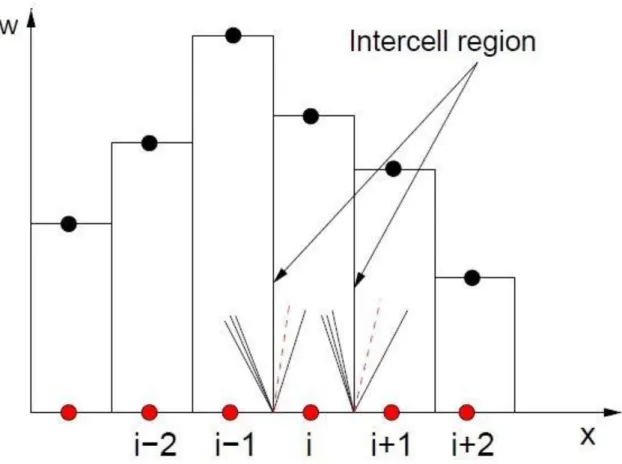
Fig. 1.6 Piecewise-constant data for Gudonov scheme ... 24
Fig. 1.7 Centered wave system generated by the Riemann problem located at the inter-cell region ... 25
Fig. 2.1 Isentropic processes depicted on an a-s diagram ... 27
Fig. 2.2 Enthalpy-entropy diagram for a turbine ... 32
Fig. 2.3 Mass flow characteristics for a turbine ... 33
Fig. 2.4 Turbine schematization ... 35
Fig. 2.5 Enthalpy-entropy diagram for a compressor ... 38
Fig. 2.6 Mass flow characteristics for a compressor ... 39
Fig. 2.7 Extended mass flow characteristics for a compressor ... 39
Fig. 2.8 Schematic diagram of turbocharger rotor ... 41
Fig. 3.1 The Cursor 11 engine on the market ... 46
Fig. 3.2 Technical data sheet Cursor 11 (353 kW) ... 47
Fig. 3.3 C11 power and torque curves ... 47
Fig. 3.4 Model of the Cursor11 implemented in GasdynPre3 ... 48
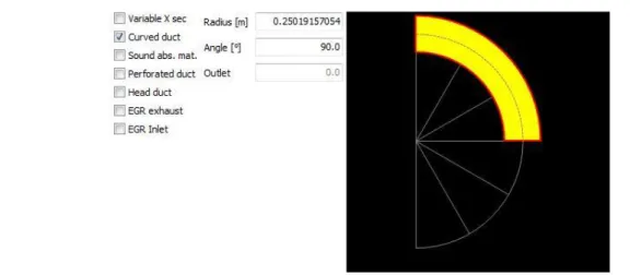
Fig. 3.5 GasdynPre3, duct options: curved duct ... 50
Fig. 3.6 GasdynPre3, duct options: output ... 51
Fig. 3.7 GasdynPre3, filter cartridge panel ... 53
Fig. 3.8 GasdynPre3, cylinders panel: geometry ... 54
Fig. 3.9 Classification of combustion models ... 55
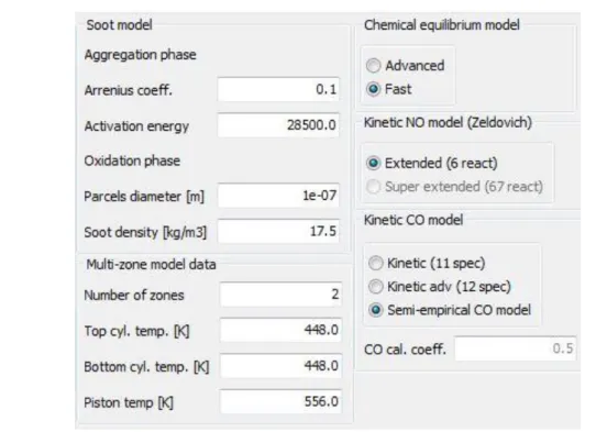
Fig. 3.10 GasdynPre3, emissions panel ... 58
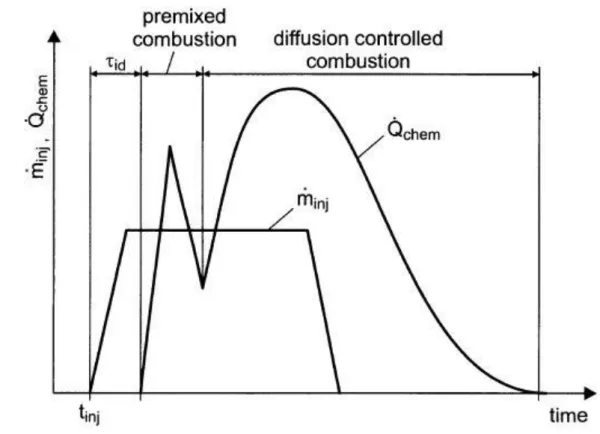
Fig. 3.11 Schematic representation of the combustion in a Diesel engine ... 60
Fig. 3.12 Short Route EGR ... 61
Fig. 3.13 Throttle body ... 61
Fig. 3.14 GasdynPre3, turbine maps (opening 100%) ... 63
Fig. 3.15 GasdynPre3, compressor maps ... 64
Fig. 3.16 Engine speed vs BMEP, provided by FPT ... 66
Fig. 3.17 GasdynPre3, engine speed range panel ... 67
Fig. 3.18 GasdynPre3, fluid type panel ... 68
Fig. 4.1 Comparison on break power ... 70
Fig. 4.2 Comparison on break torque ... 71
Fig. 4.3 Comparison on bmep ... 72
Fig. 4.4 Comparison on peak cylinder pressure ... 72
Fig. 4.5 Comparison on mechanical efficiency ... 73
Fig. 4.6 Comparison on bsfc ... 74
Fig. 4.7 Pilot injection imposed in Gasdyn ... 74
Fig. 4.8 Main injection imposed in Gasdyn ... 75
iv
Fig. 4.13 Comparison on p-V diagram, B100 ... 77
Fig. 4.14 Comparison on p-CA diagram, C100 ... 78
Fig. 4.15 Comparison on p-V diagram, C100 ... 78
Fig. 4.16 Comparison on concentration of NOx ... 79
Fig. 4.17 Comparison on produced soot ... 79
Fig. 4.18 Comparison on air mass flow rate ... 80
Fig. 4.19 Comparison on boost pressure ... 81
Fig. 4.20 Comparison on compressor inlet pressure ... 81
Fig. 4.21 Comparison on compressor inlet temperature ... 82
Fig. 4.22 Comparison on compressor outlet temperature ... 82
Fig. 4.23 Comparison on compressor pressure increase ... 83
Fig. 4.24 Comparison on compressor temperature increase ... 83
Fig. 4.25 Comparison on pressure before the intercooler ... 84
Fig. 4.26 Comparison on temperature before the intercooler ... 84
Fig. 4.27 Target values of the EGR percentage set in Gasdyn PID controller ... 85
Fig. 4.28 Comparison on EGR percentage ... 86
Fig. 4.29 Comparison on EGR mass flow rate ... 86
Fig. 4.30 Comparison on the temperature before the throttle valve ... 87
Fig. 4.31 Comparison on temperature after the EGR cooler ... 87
Fig. 4.32 Comparison on exhausts mass flow rate ... 88
Fig. 4.33 Comparison on pressure before the turbine ... 88
Fig. 4.34 Comparison on temperature before the turbine ... 89
Fig. 4.35 Comparison on pressure after the turbine ... 90
Fig. 4.36 Comparison on compressor efficiency ... 91
Fig. 4.37 Comparison on compressor ratio ... 91
Fig. 4.38 Comparison on turbocharger revolution speed ... 92
Fig. 4.39 Turbocharger routine output. Starting from down left and proceeding clockwise there are: turbocharger revolution speed, behaviour of boost pressure with respect to the target value, power balance and VGT opening percentage ... 93
Fig. 4.40 Operating points of compressor (upper part) and turbine (lower part) for a determined VGT aperture ... 94
v
List of Tables
Table 1 Woschni model constants ... 57 Table 2 Family of points simulated ... 66
ix
Abstract
This thesis deals with the validation of a six cylinders, turbocharged, heavy-duty compression ignition Diesel engine equipped with a short route Exhaust Gas Recirculation system (EGR) dedicated to the truck transportation. Validate an engine means compare the parameters predicted with a simulation tool with the results of an experimental campaign. This engine is built by Fiat Power Train (FPT) that provides the data necessary for the comparisons. In particular, twelve points at different load and engine speed are considered.
The 1D Computational Fluid Dynamic (CFD) model adopted in this work is GASDYN which is a research code developed by the Internal Combustion Engine (ICE) group of Politecnico di Milano. This software is coupled with a Graphical User Interface (GUI), that, in its last version, is called GASDYNPRE3. Through this interface the scheme of the engine is drawn in all its main components to create the input files necessary to GASDYN to perform the thermo-fluid dynamic simulations.
xi
Sommario
Questa tesi riguarda la validazione di un motore Diesel di grossa taglia, turbo-sovralimentato a sei cilindri, con un circuito per la ri-circolazione dei gas combusti, destinato ai mezzi pesanti. Validare un motore significa confrontare i risultati dei principali parametri operativi calcolati con uno strumento di simulazione con gli stessi dati derivati da una campagna sperimentale. Il motore studiato è costruito dalla Fiat Power Train (FPT) che ha fornito i dati sperimentali necessari per i confronti. In particolare sono stati studiati dodici punti differenti per carico e giri del motore.
Il modello monodimensionale di fluidodinamica computazionale utilizzato in questa tesi è il GASDYN: un codice di ricerca sviluppato dal gruppo motori a combustione interna del Politecnico di Milano. Questo software è accoppiato ad una interfaccia grafica che, nella sua ultima versione, si chiama GASDYNPRE3. Con questa interfaccia è possibile costruire il modello del motore con tutti i suoi componenti per fornire a GASDYN i parametri di input necessari per le simulazioni termo-fluidodinamiche.
1
Introduction
Nowadays the automotive industry is living times of important changes. On one hand, a more and more restrictive emission regulation is forcing the constructors to find new solutions or to refine the already existing strategies to cope with the new and always lower limits of pollutant emissions. On the other hand, the electric world is becoming an important factor. Several technologies have been developed in the last few years: hybrid vehicles and plug-in electric vehicles to cite the two most important.
Nevertheless, the traditional gasoline and Diesel engine are far from be considered the past. In particular, for the heavy-duty vehicles (like trucks and buses) the Diesel engines represent still the best solution. Indeed, the main requests of the heavy-duty sector are the lowest possible fuel consumption and the maximum durability. To satisfy these two aspects there is not a better engine than a heavy-duty turbocharged Diesel engine, like the one studied in this thesis.
To avoid the construction and the test of many prototypes with consequent high costs, the development of different Computational Fluid Dynamic (CFD) simulation tools is of primary importance. In particular, to speed up the engine design process, the one-dimensional (1D) CFD analysis is a good compromise. Indeed, before building a prototype or even before performing a more detailed CFD analysis which needs large computational time and/or an advanced computer, a one-dimensional CFD simulation tool represents the perfect first step in the study of the complex fluid-dynamic of an internal combustion engine.
For this reason, the Internal Combustion Engine (ICE) group of the Energy Department of Politecnico di Milano has developed a one-dimensional simulation tool able to perform a sufficiently detailed analysis of the main engine parameters. This tool is GASDYN and is the software which provided all the results reported in this thesis. It is able to study the wave motion in an internal combustion engine through the numerical methods implemented in it. The code is coupled with a graphical interface called GASDYNPRE3 in the last version available. With this interface, is possible to draw a scheme of an engine considering all the typical components encountered by the fluid moving in the ducts. Indeed, pipes, junctions, valves, cylinders, intercooler, compressor and turbines can all be modeled in GasdynPre3. Some of these components can be directly drawn because there is the equivalent one-dimensional component already implemented; others components have to be modeled modifying other elements to the purpose. An example used in this work is given by the intercooler. Actually, in GasdynPre3 there is not a dedicated element to model this heat exchanger and so has been used a filter modifying some parameters.
In this Master thesis a turbocharged heavy-duty Diesel engine equipped with a short route Exhaust Gas Re-circulation (EGR) system has been studied. Firstly, a complete scheme of the engine is drawn and detailed in GasdynPre3. Then, the results of the main engine parameters computed by Gasdyn are compared with the correspondent data provided by the constructor (Fiat Power Train).
In the first chapter, a review of the governing equations of the fluid motion in a duct is provided in the first part. Then, some numerical methods actually implemented in Gasdyn are presented. The first method presented is the Method of Characteristics which was the dominant method in the past and is the model for the most advanced numerical methods implemented in the simulation tool. In particular two second-order, space-centered, finite differences methods are detailed. Since these method are of second-order accuracy they
2
suffer the problem of spurious oscillations that will be explained. So, they are coupled with two possible flux limiting techniques. In addition to these second-order methods, in Gasdyn is implemented also the explicit, first-order, Gudonov type method (upwind) based on the HLLC Riemann solver.
In the second chapter, the turbocharger is described from the point of view of the numerical analysis. Indeed, the elements that are between two pipes represent the boundary conditions of the numerical methods. The turbocharger is the most complex boundary condition. In this chapter the strategy used in Gasdyn to model this component is presented, starting from the turbine and continuing with the compressor. The chapter is closed with the description of the turbo-matching: the achievement of the balance between the power produced by the turbine and that absorbed by the compressor.
The third chapter deals with the modelling of the engine in GasdynPre3. Firstly, the real engine is presented, specifying that is not exactly the same studied in this work. Indeed, the EGR system present in the prototype studied is absent in the engine actually on the market because FPT has developed a system able to reduce the pollutants without the EGR. The strategy used to model each component is explained in detail, specifying the source of the input data like geometry or the heat transfer properties of the material.
In the fourth chapter, the validation process is described. Starting from the main engine operating parameters, the results computed by Gasdyn are compared with the data provided by FPT. The work will end with the analysis of the main turbocharger parameters performed with a Matlab routine developed always by the ICE group.
3
1 Governing Equations and Numerical Methods
Introduction
1.1
Being volumetric machines, the internal combustion engines are characterized by unsteady flows both in the inlet and in the outlet section. To model properly this type of machine, mathematical models able to reproduce the wave motion of the flow are necessary.
In this first chapter the governing equations and the numerical methods implemented in Gasdyn, and thus used to develop this theses, are presented.
Starting from the governing equations describing the one-dimensional flow in a pipe, a list of hypothesis is presented. These hypothesis are useful to obtain a proper formulation to model the flows in the engines ducts.
In the second part of the chapter the numerical methods are presented. First, the Method of Characteristics is explained. This method dominated the field until the 1950s, when finite differences (or finite volumes) methods started to be developed. Then, Shock-Capturing methods and a particular form of Riemann solver implemented in Gasdyn are presented.
Governing Equations
1.2
The cyclic opening and closing of the engine valves produces important pressure and velocity variations in the fluid moving in the ducts and in the cylinders. These processes are strongly unsteady: temperature and entropy gradients are significant and the fluid shows heavily its compressibility and viscosity. The most complete mathematical description of the flow of the fluid are the Navier-Stokes equations in three dimensions, supplemented by empirical laws relating the dependence of viscosity and thermal conductivity to the other flow variables, and by thermodynamic state relationships. With current computing power these equations can be solved directly only for extremely simple flow cases. The complexity of this approach and the huge computational time necessary to run the simulations has brought to the development of one dimensional models. [1] [2]
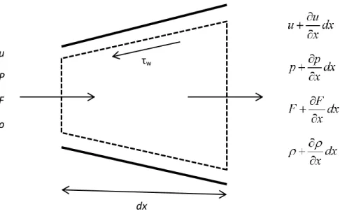
Considering Fig. 1.1, the continuity, momentum and energy equation are developed for the control volume depicted in dotted lines. The one dimensional study is based on a series of assumptions:
1. Unsteady flow;
2. Compressible fluid: it is adopted the perfect gas model with constant specific heat or the ideal gas model with specific heat dependent on composition and temperature;
3. One-dimensional flow: the fluid dynamic quantities (pressure p, fluid velocity u, density ρ) are considered constant in the cross section and function only of the curvilinear abscissa x, taken generally along the duct axis, and the time variable t. This assumption is valid because the length to diameter (L/D) ratios of the pipes are large enough for the flow to be fully developed turbulent flow; 4. Variable cross section: small variations of the section area, F;
4
6. Inviscid fluid: the gas is sufficiently “dilute” for the internal stresses to be ignored;
Assuming valid these hypothesis, the Eulerian approach is adopted.
Fig. 1.1 Control volume for variable area flow o Continuity Equation
The net rate of flow out of the control volume equals the rate of decrease in mass in the control volume:
u dF dx u dx F dx uF Fdx x x dx t (1.1)Considering only first-order small quantities and rearranging:
0 u u dF u t x x F dx (1.2)
u u dF 0 t x F dx (1.3) o Momentum EquationThe resultant of pressure forces and shear forces on the control surface equals the sum of the rate of change of momentum within the control volume and the net efflux of momentum out of the control surface.
u P F ρ τw dx
5 - The pressure forces on the control surface are equal to the sum of the forces on the end faces and the forces on the side walls; all forces are assumed positive in the x-direction:
p dF dF dF pF p dx F dx p dx pF dx p dx x dx dx x dx (1.4)The first two terms consider the pressure on the end sections while the third represents the effect of the pressure component along the x direction on the lateral surfaces of the control volume;
- The shear forces are due to the friction at the wall 2 2 w u Ddx f Ddx (1.5)
where D is the equivalent diameter (in case of variable or rectangular shape cross section) and the wall shear stress τw is related to the friction factor f by the
expression: 2 1 2 w f u (1.6)
- The rate of change of momentum in the control volume is
Fudx
t
(1.7)
- Considering only first order small quantities the net efflux of momentum from control surface is
2 2 2 u dF dx u dx F dx u F u F dx x x dx x (1.8)Hence the momentum equation is
2
2
2 dF u pF dx p dx f Ddx Fudx Fu dx x dx t x (1.9)Expanding, diving by F and changing sign gives 2 4 0 2 u u dF u p u u u u f u t x F dx x D x t x (1.10)
The term in the bracket is identically zero, from the continuity equation. Hence the momentum equation becomes
1 0 u u p u G t x x (1.11) where 2 4 2 u u G f u D (1.12)
6
o Energy Equation
The energy equation can be derived by applying the First Law of Thermodynamics to the control volume in the form
0 0 S E H Q W dx t x (1.13)
where E0 is the total stagnation internal energy of the control volume and H0 is the
total stagnation enthalpy. The first term in the right-hand side can be written in terms of the specific stagnation internal energy as
0
0 e Fdx E t (1.14) where e0 is defined as 0 2 1 2e e u . The second term on the right-hand side of the equation represents the net efflux of stagnation enthalpy across the control surface and is given by
0
0 h Fu H dx x (1.15)where h0 is the stagnation enthalpy of the fluid, which is related to the stagnation
internal energy by the equation 0 0
p h e
(1.16)
Radial heat transfer from the gas to the manifold wall, or viceversa, is easily incorporated into the energy equation. Using the convention that the heat transfer is positive into the control volume, if the heat transfer rate per unit time per unit mass of gas is denoted as q and the heat released per unit volume per unit time by possible chemical reactions in the exhaust manifold is denoted as qHR, then the total
heat transfer rate from/to the control volume is [3]
HR
Qq Fdx q Fdx (1.17) The work done by or on the system, W , is zero for gas flow in a pipe element of an S engine manifold. In terms of the above quantities the energy equation takes the form
0
0
HR e Fdx h Fu q Fdx q Fdx dx t x (1.18)To summarize, the governing equations for the one-dimensional flow of a compressible fluid in a pipe with area variation, wall friction, and heat transfer are a set of non-linear hyperbolic partial differential equations
7
0
0
0 1 0 HR u u dF u t x x F dx u u p u G t x x e Fdx h Fu q Fdx q Fdx dx t x (1.19)These equations contain the four unknows ρ, u, p, and e. A further relationship is required to solve the problem. The properties of the gas must be related by a state equation: for the gases in engine manifolds and cylinders the ideal gas state equation is usually sufficiently accurate. Moreover, if the fluid is considered to be a perfect gas the internal energy can be expressed as the product of specific heat capacity at constant volume and the temperature. These properties are summarized by these two equations:
p RT
(1.20)
v
ec T (1.21)
With these assumptions it is possible to re-write the energy equation substituting the internal energy e:
2
2 2 2 HR v v u p u q Fdx q Fdx Fdx c T uF c T dx t x (1.22)Rearranging this last equation and combining it with the continuity and momentum equation, the energy equation in non-conservation form is obtained:
2 1 qHR 0 p p u a u k q uG t x t x (1.23)Where a is the speed of sound, that for a perfect gas is a kRT and k is the ratio of specific heats at pressure and constant volume p
v
c k
c
Modern finite volume methods for solving the equations of compressible flow can be based on the conservative form derived below, but the more traditional Method of Characteristics is based on the non-conservative form of the equations:
2 0 1 0 1 HR 0 u u dF u t x x F dx u u p u G t x x q p p u a u k q uG t x t x (1.24)8
The equations can be expressed in a manner which conserves the properties of the fluid in pipes with varying cross-section area. In this way the conservative form is derived:
2 2 0 0 0 1 0 2 0 HR F uF t x u p F uF dF p u f D t x dx e F uh F q F q F t x (1.25)This formulation permits to describe the discontinuities in the flow. To write the conservative form it is necessary to identify the groups of variables conserved through the shocks and collect them in a common differential operator.
This set of equations can be re-written in symbolic vector form, useful for the application of the Shock-Capturing methods. If the cross-sectional area is retained in differential terms, the governing equations become:
,
0 F W W x t C W t x (1.26)Where the three vectors are:
1.
0 , F W x t uF e F vector of convective fluxes.
2.
2
0 uF F W u p F uh F vector in x-direction. 3.
0 0 0 HR dF C W p GF dx q q F vector of source terms
where the first part contains the pressure force source terms due to the section variation while the second part considers the effects of the friction and the heat exchanges.
As noted for the equations in non-conservative form, also in this case a state equation is required.
9
Numerical Methods
1.3
In general, it is not possible to obtain analytical solutions for the hyperbolic partial differential equations derived in the previous paragraph and numerical techniques have to be developed. Basically, it is necessary to discretize the governing equations to form a set of algebraic relationships which can then be solved on a computer.
The Method of Characteristics was the dominant numerical technique in the area of simulating the gas dynamics processes in engine manifolds. This method is exploited in Gasdyn to define the boundary conditions: the turbocharger case is shown in the next chapter. While this method is still extremely powerful in formulating boundary conditions it has been superseded in the pipes themselves by modern finite difference/volume schemes. Such techniques are based on the conservative form of the governing equations and provide discretizations which explicitly preserve the transport of mass, momentum and energy.
Shock Capturing schemes apply the same numerical algorithm throughout the flow field. In this work the methods implemented in Gasdyn are presented. In particular two second-order shock-capturing finite difference methods are described. Godunov shows that schemes with greater than first-order spatial accuracy generate spurious oscillations that can be mitigate through specific techniques.
The final part of the chapter is dedicated to the description of a first-order Riemann solver. Due to its good robustness coupled with a high calculation velocity, it is indicated when the number of simulations is important, as in this thesis.
1.3.1 Method of Characteristics
The Method of Characteristics was the first numerical technique used to solve the set of hyperbolic partial differential equations presented in the previous paragraph. The main ability of this method is the possibility to transform the system of partial differential equations in ordinary differential equations along particular lines, called characteristic lines.
This method presents three important limits. At first, it deals with the assumption of perfect gas. Then it uses a linear approximation to discretize the space-time domain to determine the physical quantities between different point of the mesh. In this way the solution is determined with a first order accuracy between two consecutive points. The last limit is its inability to convey true discontinuities at the correct speed.
As already stated the Method of Characteristics deals with the non-conservative form of the governing equations that is reported below:
2 0 1 0 1 HR 0 u u dF u t x x F dx u u p u G t x x q p p u a u k q uG t x t x (1.27)10
Considering these equations and manipulating them to highlight the following quantities (u+a), (u-a) and u, it is obtained this set of equations:
1 2 3 1 2 3 2 1 0 0 0 p p u u u a a u a t x t x p p u u u a a u a t x t x p p u a u t x t x (1.28) where
1 2 2 3 1 qHR k q uG ua dF F dx aG The first Δ term characterizes the heat transfer, it is irreversible and greater than zero in case of non-homentropic flow. The second term depends on the change of cross-sectional area along the pipe (reversible, homentropic). The last term describes the wall friction and, as the first, it’s irreversible and greater than zero in case of non-homentropic flow.
The expressions in the brackets are the ordinary differentials of the variables p, u and ρ calculated along the characteristic lines that in the plane (x,t) have the slope defined by the flow properties: dx u a dt (1.29) dx u a dt (1.30) dx u dt (1.31)
These equations are called direction equations. The characteristic speeds given by these equations represent the speed of propagation of signals through the fluid medium. In the case of the first two equations the disturbance is propagated at the local speed of sound relative to the fluid u+a (right-running wave) and u-a (left-running wave). Such a disturbance is called wave characteristics and causes changes in the fluid pressure, density, temperature and velocity. The third equation is called pathline characteristic and represents a disturbance propagating with the local fluid velocity u, which transports the bulk gas energy level and composition.
A characteristic line in the plane (x,t) divides the plane in two regions in which the fluid dynamic quantities differ for infinitesimal values, but their derivatives show finite differences.
Direction equations that define the characteristic lines permit to evaluate the equations (1.28) along these lines and the partial differential equations become ordinary differential equations and are called compatibility equations.
11 Along the characteristic lines, the resulting total differentials are:
dp p p u a dt t x (1.32)
du u u u a dt t x (1.33) dp p p u dt t x (1.34) d u dt t x (1.35)Substituting these differentials in the equations (1.28), the compatibility equations can be obtained: 1 2 3 1 2 3 2 1 0 0 0 dp du a dt dt dp du a dt dt dp d a dt dt (1.36) Or equivalently
1 2 3 1 2 3 2 1 1 1 0 1 1 0 0 dp du dt a a dp du dt a a dp a d dt (1.37)The first two equations relates the pressure and the velocity of the gas along the characteristics defined by the equations (1.29) and (1.30). Similarly the third relates the pressure and the density along the characteristics defined by equation (1.31).
Homentropic Flow
To simplify the discussion, initially the cross section is constant and the flow is considered homentropic: there is no heat transfer and or wall friction and the entropy level of the fluid remains constant. The homentropic approach can be a good approximation of the flow in the intake manifolds, where the energy and entropy levels of the gas do not vary greatly. With this hypothesis the equations become:
12 2 1 0 1 0 0 dp du a dp du a dp a d (1.38)
The Second Law of Thermodynamics states: dp Tds dh
(1.39)
For an isentropic process ds=0 and hence
dpdh (1.40)
The enthalpy of a perfect gas can be expressed as 2 1 1 p kRT a h c T k k (1.41)
which can be differentiated to give 2 1 a dh da k (1.42)
Substituting this equation in equation (1.40) and then in the first two equations of (1.38) gives: 1 0 2 1 0 2 k da du k da du (1.43)
This set can also be written as:
1 0 2 1 0 2 k d a u k d a u (1.44)
The terms in the brackets are called Riemann invariants in case of homentropic flow because they are constant along the wave:
1 1
2 2
k k
a u a
(1.45)
Writing that λ and β are constant in case of homentropic flow means that travelling from point 1 to point 2 along the wave it is 1 2
These equations can be represented in a graphical way with the correlated direction equations in two diagrams called position diagram and state diagram:
13 Fig. 1.2 Position diagram (a) and state diagram (b)
The gas velocity and the speed of sound can be obtained adding and subtracting each other equations (1.45) to give
2 a (1.46) 1 u k (1.47)
The physical significance of the above equations can be appreciated by considering the following figure where the direction equations are depicted in a regular orthogonal grid at intervals of Δx and Δt:
Fig. 1.3 Homentropic characteristics
The value of the mesh size used in a computation is determined by the user. The value of the time step, however, is subject to constraints imposed through stability considerations which arise from the criterion of Courant, Friedrichs and Lewy (CFL). This criterion
Δx Δt L R Tim e, t Distance, x n+1 n i-1 i i+1
14
requires that waves cannot travel more than one mesh length in one calculation time increment. This is expressed through this equation:
max in in 1 i t CFL u a x (1.48)The rightward propagating wave travelling at speed u+a sets off from point L at time level n and arrives at point i at time level n+1. Similarly the leftward travelling at speed u-a originu-ates u-at point R u-at time level n u-and u-arrives u-at point i u-at time level n+1. If the gu-as velocity is not zero the point L is not at same distance from the mesh point I as point R.
Due to what written above, for a rightward moving wave it can be stated
1 1 1 1 1 2 2 n n n n n n i L i i L L k k a u a u (1.49)
where the subscript denotes the spatial position and the superscript denotes the time level to which the variables refer.
Likewise, for a leftward moving wave
1 1 1 1 1 2 2 n n n n n n i R i i R R k k a u a u (1.50)
These two last equations define the values of the quantities a and u at mesh point i at the new time level n+1 starting from their value at the points L and R. The values at points L and R are obtained by linear interpolation of the values at [(i-1),n], [i,n] and [(i+1),n], thus producing first-order spatial accuracy.
A time marching procedure can be used in a computer simulation program where the values of the gas properties at the new time level are completely determined by the values at the previous time level at every point in a pipe that is surrounded by two other points.
At boundaries, the values of the gas properties in the pipe are available on only one side of the mesh point under consideration and a modified procedure must be adopted. Typical boundaries for which methods exist are: open ends, closed ends, inflow boundaries and valve boundaries. Benson describe how to cope with all these boundaries. The treatment of all these has one feature in common: the boundaries are all treated as if the flow is quasi-steady. This assumption implies that the physical size of the boundary can be neglected compared with the length of the pipe connected to it and that the equations of steady flow can be applied locally to this infinitesimally small region.
Non-Homentropic Flow
The general solution to flow in pipe systems takes into account variation in the entropy level of the gas. In order to transform the first two compatibility equations of (1.37) in the equivalent of the equations (1.43) the Second Law of Thermodynamics is rearranged
dp dh Tds
a a a
(1.51)
15
1 2 3 1 2 3 1 1 1 0 2 2 2 1 1 1 0 2 2 2 k k k T da du ds dt a a k k k T da du ds dt a a (1.52)This equation shows that the Riemann “invariants” are not constant in non-homentropic flow and in fact they are called Riemann variables. The variations of λ and β are given by the equation above as
1 2 3 1 1 2 2 k T k d ds dt a a (1.53)
1 2 3 1 1 2 2 k T k d ds dt a a (1.54)Since dλ and dβ are not equal to zero for non-homentropic flow the Riemann variables are modified as they traverse the flow field. In the following figure all the three direction equations are represented:
Fig. 1.4 Non-homentropic characteristics
The Riemann variables at mesh point i at time level n+1 are defined as 1 n n i L d L (1.55) 1 n n i R d R (1.56)
The Riemann variables at points L and R can be evaluated by linear interpolation between the surrounding mesh points, since the solution at the current time level n is known at each mesh point. Thus Ln and Rn are given by
1
n n L n n L i i i x x (1.57) Δx Δt L R Tim e, t Distance, x n+1 n i-1 i+1 S i16
1
n n R n n R i i i x x (1.58)Note that the value of xR x is negative if the positive x-direction is from left to right. In the following only the λ characteristic is considered, but the procedure is the same also for the β characteristic.
To calculate the gradient xL x is necessary to compute the quantity xL t which is given by n n L L L x u a t (1.59)
Substituting equation (1.46) and (1.47) in this equation gives
1 2 n n n n L L L L L x t k (1.60)
which can be written as
n n L L L x a b t (1.61)
where a and b are two constants dependent from the gas nature:
1
3
2 1 2 1 k k a b k k (1.62)Now, Ln can be expressed in the same way as Lnas
1
n n L n n L i i i x x (1.63)Substituting (1.57) and (1.63) in equation (1.61) and rearranging, the gradient xL x can be expressed in term of all quantities known at time level n:
1
1
n n i i L n n n n i i i i a b x x x a b t (1.64)The value of Ln can now be evaluated through equation (1.57). The other terms in equation (1.53) can be evaluated at point L with the same linear interpolation.
However, a different method is required to evaluate the change in entropy along the wave characteristics. This quantity can be obtained by using information available from the pathline characteristic shown in the figure above.
Starting from the pathline characteristic equation it can be demonstrated that the change in entropy level along the pathline can be expressed as
HR S q q uG ds dt T (1.65)
Thus the change in the entropy level along a pathline is due only to the heat transfer and pipe wall friction terms in the governing equations. The gas velocity at point S is given by
17 1 n n n S S S S x u t k (1.66)
and the terms on the numerator are given by linear interpolation as before
1
n n S n n S i i i x x (1.67)
1
n n S n n S i i i x x (1.68)Combining these two equations with equation (1.66) and rearranging it is obtained
1
1
1
n n S i i n n n n i i i i x x x k t (1.69)Finally the entropy level at point S can be obtained from
1
n n S n n S i i i x s s s s x (1.70)The quantities q, qHR, G and T can be calculated in the same way. Evaluating the
entropy change along the pathline with equation (1.65), the entropy level at the time level [i, n+1] can be calculated as
1
n n i S S
s s ds (1.71)
The change in entropy along the wave characteristic in equation (1.53) is given by 1
n n L i L
ds s s (1.72)
where s is given by linear interpolation at point L. Ln
Remember that the same procedure can be adopted also for the other Riemann variable expressed by equation (1.54).
1.3.2 Shock Capturing Schemes
Shock waves can occur in the exhaust manifold of high performance engine. As written in the presentation of the Method of Characteristic that method cannot deal with shock waves correctly since it is not based on the conservative form of the governing equations. The solution are numerical methods that can be applied to both smooth and discontinuous regions of the flow.
The governing equations are written in integral conservative form across a control volume. In this way they are conserved through the control volume, irrespective of the presence of discontinuities. Schemes based on this approach can therefore be expected to be valid for flows containing discontinuities because the integral form does not demand the existence of derivatives.
Through the divergence theorem the integral form of the governing equations (1.26) can be written as
18
,
0 x t F W W x t C W dxdt t x
(1.73)Omitting the source terms, C W
, and integrating, is obtained
1
1
1 2 1 2 0 1 2 1 2 n n n n n n n n i i i i i i i i t W W x F F t W W F F x (1.74)where the vector W and F are obtained through the mean value theorem as 1 1 2 1 2 1 2 1 1 n i n i x t i i x t W Wdx F Fdt x t
(1.75)The left-hand side of equation (1.74) represents the solution at the new time level n+1, and the first term on the right-hand side represents the solution at time level n.
In the following the two second-order accurate numerical methods actually implemented in Gasdyn are presented.
Lax-Wendroff Schemes
The Lax-Wendroff method is based on the Taylor expansion for the state vector W as
2 2 1 2 2! n n W W t W W t t t (1.76)Equation (1.26) with the source term equal to zero gives
W F t x (1.77) and 2 2 W F F t t x x t (1.78) but F F W F F F A t W t W x x (1.79)
where A is a 3x3 Jacobian matrix consisting by elements defined by
i ij j F a W (1.80) Hence 2 2 W F F A t x t x x (1.81)
19
2
1 3 2! n n F F t W W t A O t x x x (1.82) Or equivalently
2
1 2 3 2! n n W W t W W A t A O t x x x (1.83)Approximating the spatial differences with the central differences and considering the matrix A constant the final form of the Lax-Wendroff method is:
2 1 2 1 1 1 1 1 2 2 2 n n n n n n n i i i i i i i t t W W A W W A W W W x x (1.84)
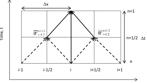
The previous derivation of the Lax-Wendroff equations required the evaluation of the Jacobian matrix. Richtmyer proposed an approach which removed the need to calculate this matrix, while retaining second-order accuracy, by solving the equations in a two-step approach.
In the first step, known the value of the vector F and W at time level n in the points i-1, i and i+i-1, the value 1 21 2
n i
W are calculated through a first order Taylor expansion:
1 2 1 1 2 1 1 2 2 n n n n n i i i i i t W W W F F x (1.85)
1 2 1 1 2 1 1 2 2 n n n n n i i i i i t W W W F F x (1.86)In the second step, the values of 1 21 2
n i
F are obtained using the values of
1 1
n i
W and the
value of the vector W at time level n+1 in point i
1 1 2 1 2 1 2 1 2 n n n n i i i i t W W F F x (1.87)20
Fig. 1.5 Computational stencil for two-step Lax-Wendroff scheme MacCormack Scheme
The MacCormack method is another second-order accurate scheme that uses alternate forward and backward spatial differences for the two steps in space. These steps are referred to a ‘predictor’ phase and to a ‘corrector’ phase respectively.
If in the first step forward differencing is used to obtain an intermediate value of W*
gives * 1 0 n n n i i i i W W F F t x (1.88)
The second step then uses backward spatial differencing while advancing over a time interval t 2 as
1 1 2 * 1 0 1 2 n n n i i i i W W F F t x (1.89) where 1 2 1
*
2 n n i i i W W W The method is used in the form
* 1 n n n i i i i t W W F F x (1.90)and the final solution is
1 * * * 1 1 2 n n i i i i i t W W W F F x (1.91)The stability of the scheme at discontinuities is influenced by the direction of the spatial differencing used in each of the steps. The “forward predictor/backward corrector” scheme given above is best suited to handling discontinuities which propagate from left to right,
n+1/2 Δx Δt Distance, x Tim e, t i-1 i i+1 n+1 n i-1/2 i+1/2
21 whereas a “backward predictor/forward corrector” scheme will be more suitable for discontinuities travelling in the opposite direction. In unsteady flow calculations (like the case of an engine) the propagation direction of discontinuities can change with time and is generally not known at any instant, hence it is usual to reverse the order of the spatial differences between each time step.
1.3.3 Spurious Oscillations and Mitigation Techniques
It is found that all the second-order space centred difference schemes generate spurious oscillations when severe gradients in the initial data, such as shock waves or contact surfaces, are encountered. In fact, it was shown by Gudonov that schemes with constant coefficients (linear schemes) giving greater than first-order spatial accuracy generate spurious oscillations at discontinuities. This is the so-called Gudonov’s theorem.
Some criterion is required to establish if schemes suffer or not from spurious oscillation. A very tested criterion is the total variation diminishing (TVD) principle. The total variation of solution w at the time n is defined by
1n n n
i i i
TV w
w w (1.92)If the total variation of the solution does not increase from one time step to the next then
n 1
nTV w TV w (1.93)
and the data are said to be total variation diminishing. A numerical scheme that generates data which satisfies this criterion will not produce spurious oscillations at discontinuities.
There are two classes of numerical methods for achieving the total variation diminishing condition with high-order accuracy:
1. Post-processing schemes: involve calculating the solution using a suitable numerical method and then modifying it to satisfy the TVD criteria.
2. Pre-processing schemes. Modify the data representation prior to updating the solution.
In Gasdyn two ways to mitigate the problem of spurious oscillations through post-processing schemes are implemented.
Flux Limiters: TVD
To explain the main idea of the flux limiters a simple model equation is taken as starting point. This is the so-called linear advection equation that is a first-order equation with which to test numerical schemes:
0 w w a t x (1.94)
It characterizes a propagation phenomena in the x-direction at velocity a. For this equation the one-step Lax-Wendroff method can be rewritten in the form
1 1/2 1/2 1 1 _ 2 n n n n i i i i w w CFLw CFL CFL w (1.95) where CFL a t x is the Courant, Friedrichs and Lewy criterion that must be less or