Benchmarking of event triggered control algorithms

(1)

POLITECNICO DI MILANO

SCHOOL OF INDUSTRIAL AND INFORMATION

ENGINEERING

Master of Science in Automation and Control Engineering

BENCHMARKING OF EVENT TRIGGERED

CONTROL ALGORITHMS

Supervisor:

Prof. Alberto LEVA

Graduation Thesis of:

Hikmet GULER, matricola 894019

(2)

(3)

iii

(4)

(5)

v

Acknowledgments

I would like to thank Prof. Alberto Leva, who has guided me and been a mentor to me during this project.

Also, I would like to thank my father, my mother, my brother and my sister for their support along with all my life. Furthermore, I thank my friends who are always on my side.

(6)

(7)

vii

List of Figures

Figure 1: General schema of a control system ... 17

Figure 2 Block diagram of the event-based control system ... 19

Figure 3: Send on Delta graph ... 22

Figure 4: Definition of relative dead-band ... 23

Figure 5: Integral sampling of energy ... 24

Figure 6: Simulation with send on delta method ... 25

Figure 7: Simulation with integral sampling of energy method ... 25

Figure 8: An example chart of hysteresis relay ... 26

Figure 9: Behavior of SSOD control system ... 26

Figure 10: PID class ... 28

Figure 11: PID struct data type ... 28

Figure 12: tf struct ... 28

Figure 13: Update functions ... 29

Figure 14: Revert functions ... 29

Figure 15: Calculation functions ... 29

Figure 16: Flow chart of OOP PID ... 30

Figure 17; Front panel and block diagram in LabVIEW environment ... 31

Figure 18: Calculation case ... 32

Figure 19; inside of the calculation subvi ... 33

Figure 20: Event generator vi’s front panel and block diagram ... 35

Figure 21: PID cluster ... 36

Figure 22: Transfer function cluster ... 36

Figure 23: Constant send on delta subvi’s block diagram ... 37

Figure 24: Relative send on delta subvi’s block diagram ... 37

Figure 25: Integral sampling subvi’s block diagram ... 38

Figure 26: Send on energy subvi’s block diagram ... 39

Figure 27: Symmetric send on energy subvi’s block diagram ... 40

Figure 28:Set point given in the C++ environment ... 42

Figure 29: Control signal in C++ environment ... 42

Figure 30: System output in C++ environment ... 43

Figure 31: Control signal in Labview environment ... 44

Figure 32: System output in Labview environment ... 45

(10)

x

Figure 34: Output of the 1st _{order system using constant dead-band method ... 47}

Figure 35: Output of the 1st _{order system using relative dead-band method... 47}

Figure 36: Output of the 1st _{order system using integral sampling method ... 48}

Figure 37: Output of the 1st _{order system using send-on-delta method ... 48}

Figure 38: Open-loop step response of the 2nd_{order system ... 50}

Figure 39: Output of the 2nd _{order system using constant dead-band method ... 51}

Figure 40: Output of the 2nd _{order system using relative dead-band method ... 51}

Figure 41: Output of the 2nd _{order system using integral sampling method ... 52}

Figure 42: Output of the 2nd _{order system using send-on-delta method ... 52}

Figure 43: Output of the 2nd _{order system using symmetric send-on-delta method ... 53}

Figure 44: Step responses for the triggering mechanisms for G1 ... 55

Figure 47: Step responses of the triggering mechanisms for G1 ... 58

Figure 48: Step responses of the triggering mechanisms for G2 ... 58

(11)

xi

List of Tables

Table 1: The results of the benchmarking the event triggering mechanisms with the given system above ... 49

Table 2: The results of the benchmarking the event triggering mechanisms with the given system above ... 53

Table 3: The results for the first variation of the system with multiple equal poles ... 56

Table 4: The results for the first variation of the system with multiple equal poles ... 56

Table 5: The results for the third variation of the system with multiple equal poles ... 57

Table 6: The results for the first variation of the fourth-order system ... 59

Table 7: The results for the second variation of the fourth-order system ... 60

(12)

(13)

xiii

Abstract

Nowadays, a consistent amount of sensing and actuating devices for control systems exploit wireless communication mechanisms and use accumulators as their primary energy source, bringing the battery lifecycle among the relevant aspects to be considered.

One possible technique to reduce battery consumption is making these devices execute their task – that is, transmitting samples of the process’ output or performing a control action – “only when necessary” and remaining in a low-power state for the remaining time. Event-based or event-triggered control techniques exploit this principle: in these control methods, differently from the “classical” ones, a new control action is computed and applied to the process only when its output varies from the setpoint for more than a given threshold. It is apparent, then, that the sensing device monitoring the process’ output has to transmit its measurement to the control system only when certain conditions are met. Additionally, these control techniques bring in advantages also in terms of actuator’s wear: as said before, the control action is applied to the process only when there is the necessity to steer the controlled variable back to its nominal state, keeping the actuator in its previous state otherwise.

This treatise firstly introduces event-based control and its background theory, complemented with some related topics both about event triggering mechanisms and PID control, to allow the reader to have a good overview of this technique. Then, general pieces of information about the used programing language and software are given to provide the necessary background for the subsequent chapters. Finally, the treatise presents the implementation of an event-based PID controller and a benchmarking of some event triggering mechanisms in various closed-loop systems, each of which composed of a specific PID controller and process structure.

(14)

(15)

xv

Sommario

Attualmente, una consistente quantità di dispositivi di misura e attuazione impiegati nei sistemi di controllo si basa meccanismi di comunicazione wireless e utilizza batterie come fonte di energia primaria accumulatori, il cui tempo di vita diventa un parametro da tenere in considerazione.

Una possibile tecnica per ridurre il consumo della batteria è fare in modo che tali dispositivi eseguano il loro compito – ovvero trasmettere campioni dell'uscita del processo o compiere un'azione di controllo - "solo quando necessario", rimanendo in uno stato di basso consumo per il resto del tempo. Le tecniche di controllo di tipo

event-based o event-triggered sfruttano questo principio: esse, diversamente da quelle

"classiche", calcolano una nuova azione di controllo solo quando l’uscita del processo varia rispetto al valore nominale per più di una certa soglia. È quindi evidente che il dispositivo di misura collegato all’uscita del processo deve trasmettere la sua misurazione al sistema di controllo solo in determinate condizioni. Inoltre, vengono apportati dei vantaggi anche in termini di usura dei sistemi di attuazione: anche in questo caso, l'azione di controllo viene calcolata e applicata al processo solo quando è necessario riportare la variabile controllata al suo stato nominale, mantenendo l'attuatore nel suo stato precedente in tutti gli altri casi.

In questa trattazione viene dapprima introdotto il controllo di tipo event-based e la sua teoria di base, integrata con alcuni argomenti correlati inerenti sia i meccanismi di generazione degli eventi che il controllo PID, in modo da consentire al lettore di avere una buona panoramica di questa tecnica. Quindi, vengono fornite informazioni generali sul linguaggio di programmazione e sul software utilizzato per dare al lettore tutte le conoscenze necessarie alla comprensione dei capitoli successivi. Infine, il resto della trattazione presenta l'implementazione di un regolatore PID event-based e l’analisi del comportamento di alcuni meccanismi di generazione degli eventi in diversi sistemi in anello chiuso, ognuno dei quali composto da un regolatore PID specifico e un processo avente una ben determinata struttura.

(16)

(17)

17

CHAPTER 1

1. Introduction

1.1. Event-Triggered Control

Nowadays, control systems are widespread, with a particular diffusion in electrical and mechanical industries.

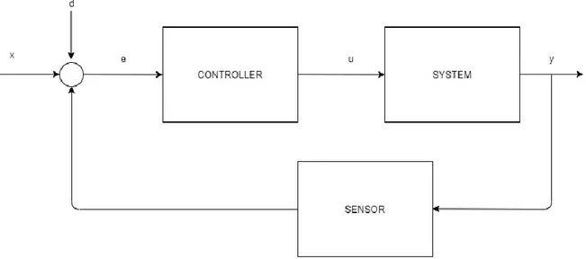
The main purpose of a control system is to supervise the behavior of a given plant or process – frequently referred to as “process” or “controlled system” – to make it meet some performance requirements, expressed in terms of settling time, maximum overshoot, maximum steady-state error, … In its general form, a control system is composed of an actuator, performing a control action on the process, a sensing unit measuring its output and a control algorithm to compute the actuator’s input basing on the measurements and the desired set-point.

Figure 1: General schema of a control system

• x: set-point value

• d: disturbance from the outside world

• u: calculated control signal (regulator’s output) • y: process’ output

(18)

18

The figure above presents the block diagram of a closed-loop system in its general form: the “system” block represents the transfer function of the controlled process, the “controller” one is in place of the controller’s transfer function – for example a PID controller. Finally, the “sensor” block represents the measurement process of the controlled system’s output.

Data transmission among the different blocks can take different forms. One of the most common methods is called periodic sampling transmission, which is employed in the fixed-rate control technique. Although based on strong theory and being a control method of simple realization, this technique may have some drawbacks. One of them is the data transmission efficiency: even when there is no necessity to measure the process’ output – i.e. when the process reached a steady-state condition - the sensor transmits its samples to the controller, occupying bandwidth unnecessarily. And, as mentioned before, this leads to premature exhaustion of the energy source in battery-powered systems. These problems can be in some way mitigated if different techniques, such as event-triggered control or aperiodic control, are used [3].

By using an event-based control technique, data exchange between sensor and controller can be limited: sensor samples are transmitted only when certain conditions are met or, in other words, “only when necessary”. An event-based control algorithm leads to numerous benefits, such as:

- reduced actuator wearing; - reduced battery consumption; - reduced computational load.

With respect to the “classical” control systems, event-based ones have one extra component, called event generator, and responsible for determining when new samples of the process’ output have to be sent to the controller. Then, the control structure comes in two forms, event-triggered control, and self-event-triggered control. The difference between those two structures is that event-triggered control is reactive and triggers event-based on the measurement of process’ output. On the other hand, in self-triggered control systems, events are generated based on a prediction of the signal evolution, according to its previous values [2].

(19)

19

The block diagram shown before, in the event-based control case, becomes the following [8]:

Figure 2 Block diagram of the event-based control system

In the figure above, the involved signals are: • w(th): control system set-point;

• u(th): control signal calculated from previous values of the process’ output and current

values of the set-point;

• u(t): continuous-time control action applied on the process by the actuator; • y(t): continuous-time process’ output;

• d(t): disturbances acting on the process;

• y(tk): samples of process’ output, according to the event-triggering mechanism.

The blocks in the above scheme are:

• Controller: here, an input for the actuator is calculated based on the actual process’ output - sampled according to the event generation rule - y(tk) and the set-point w(th).

• Actuator: here, the discrete-time control signal u(th) is converted to a continuous-time

control action u(t) applied to the process. • Plant: the controlled system.

• Sensor: in this block, the output of the system y(t) is sampled and its value is analyzed according to the event generation rule.

(20)

(21)

21

CHAPTER 2

2. Event Triggering Mechanisms

In this chapter, some event-triggered mechanisms will be analyzed. These are constant send on

delta, relative send on delta, integral sampling, send on energy and symmetric send on delta.

2.1. General Send on Delta rule

According to this rule, the event triggering law is:

𝑆(𝑡) = {1𝑖𝑓|𝑥𝑙𝑠− 𝑥(𝑡)| ≥ 𝛿

0𝑖𝑓|𝑥_𝑙𝑠− 𝑥(𝑡)| ≤ 𝛿 (2.1)

where:

• S(t): triggering function;

• x(t): the current value of the observed variable;

• xls: reference value, namely the one assumed by the observed variable the last time an

event was triggered;

• δ: event-triggering threshold, also referred to as “dead-band”.

The triggering rule is the following: if the absolute value of the difference between the reference value xls and the current value x(t) exceeds the threshold, the conditions to generate an event

(22)

22

In the following figure a graphical view of the rule behavior is provided [1]:

Figure 3: Send on Delta graph

There are many types of send on delta method, but in this project, constant dead-band send on delta method and relative send on delta method will be focused.

2.1.1. Constant Dead Band method

Here, the value for the dead band Δ is kept constant. Then, when the value recently sent is to exceed the dead band, the system changes the output.[4]

|𝑢_𝑙(𝑡)| ∈ {[0, |𝑢𝑙(𝑡′)| + ∆]𝑖𝑓|𝑢𝑙(𝑡′)| < ∆ [|𝑢𝑙(𝑡′)| ± ∆]𝑖𝑓|𝑢𝑙(𝑡′)| ≥ ∆

(2.2) The consistency between the sent value and the current value is guaranteed by this formula.

(23)

23

2.1.2. Relative Dead Band method

This method differs from the constant dead-band one by the way in which the dead band is computed. The dead band is given by the following equation:

∆_𝑢 𝑙(𝑡′)= 𝜖 ∗ |𝑢𝑙(𝑡 ′_)| _(2.3) Where: • ϵ: scale factor; • ul: control signal;

• Δ: dead band threshold.

In the practice, a minimum value for the dead band Δmin is given to prevent Δ having an

infinitesimally small value. This happens because, around the origin, the control signal ul tends

to become infinitesimally small [5].

𝛥 > 𝛥_𝑚𝑖𝑛 (2.4)

Figure 4: Definition of relative dead-band

In this case, the send function is: |𝑢𝑙(𝑡)| ∈ { [0, |𝑢𝑙(𝑡′)| + ∆𝑚𝑖𝑛]𝑖𝑓|𝑢𝑙(𝑡′)| < ∆𝑚𝑖𝑛 [|𝑢𝑙(𝑡′)| ± ∆𝑢𝑙(𝑡′)] 𝑖𝑓|𝑢𝑙(𝑡 ′_{)| ≥ ∆} 𝑚𝑖𝑛 (2.5)

2.2. Integral Sampling method

The send on delta algorithms might have some difficulties in detecting the presence of oscillations or a steady-state error if their value is smaller than the dead band. In these cases, the usage of the energy sampling error gives more accurate results [6].

(24)

24

In the integral sampling method, an event is generated when the time integral of the difference between the currently observed value and the previous one becomes greater than a given, and constant, threshold.

Figure 5: Integral sampling of energy

Where the equation used to compute the error is:

∫𝑡𝑖 (𝑥(𝑡) − 𝑥(𝑡_𝑖−1))𝑑𝑡

𝑡𝑖−1 = 𝜉 (2.6)

2.3. Send on Energy method

This method differs from the previous one by computing an area instead of an error. It also keeps the same benefits brought about by the integral sampling method with respect to the send

on delta ones.

∫𝑡𝑖 (𝑥(𝑡) − 𝑥(𝑡_𝑖−1))2𝑑𝑡 = 𝜉

(25)

25

The following figures, taken from [6], give a visual comparison between integral sampling and

send on energy methods against the send on delta ones:

Figure 6: Simulation with send on delta method

Figure 7: Simulation with integral sampling of energy method

It can be noticed that, when the steady-state error is smaller than the send on delta threshold, the control system cannot detect and correct the residual error, while the system using the

(26)

26

2.4. Symmetric Send on Delta method

Symmetric send on delta method (SSOD) belongs to the family of send on delta methods [7]. Here, the triggering mechanism is similar to the one of a relay with hysteresis. An example of which is represented in the following figure:

Figure 8: An example chart of hysteresis relay

While here the behavior of the SSOD method is presented:

Figure 9: Behavior of SSOD control system

The triggering function of this method is [9]:

(27)

27

CHAPTER 3

3. Implementation of Controller and Event

Triggering Algorithms

In this project, programming an object-oriented PID control has chosen as a starting point of the implementation. As a next milestone, the implementation of the PID controller with a similar approach used for previous PID controller implementation in the LabVIEW environment was decided. As a final step of this project, applying event-triggered control methods to a system with usage of the PID controller implemented is aimed. In related parts, some complementary information about the programing language, environment, and approach used in this project will be given.

3.1. Implementation of PID Controller in C++

Language with Object-Oriented Approach

3.1.1. C++ Programming Language and Object-Oriented

Programming Approach

C++ programming language is one of the most used programming languages. It was been developed as an extension of C programming language but on the other hand, it is designed to be more efficient and more flexible language but also able to provide high-level features for the programming world. One of those features is that it makes the usage of the classes and objects available.

Object-oriented programing is a programming paradigm used in different programming languages besides C++ and based on two fundamental concepts, which are objects and classes. Classes define specific data types, each of them having a given set of variables and methods acting on them. On the other hand, an object is an instance of classes.

(28)

28

3.1.2. Implementation of OOP PID Controller

This section presents the classes, methods, and objects used to describe an object-oriented PID controller implementation. The requirements for the implementation are:

- Get some parameters, essentially the set-point and ones for regulator tuning, from user input;

- Update the aforementioned parameters whenever requested by the user;

- Store the old set-point and tuning parameters to give the user the possibility to revert to the latest known situation whenever is necessary;

- Compute the values for the controlled variable according to the given set-point and tuning parameters.

The design of the algorithm can be summarized as follows:

To be able to get user input data and store them, the PID class contains some ad-hoc variables. The following figure shows the class definition and its properties:

Figure 10: PID class

Some other additional data types have been defined, also:

Figure 11: PID struct data type

(29)

29 The functions to update and revert parameters are:

Figure 13: Update functions

Figure 14: Revert functions

While the ones used to compute a new control action are:

Figure 15: Calculation functions

In the “isa_pid_struct” method, the tuning variables for the PID controller are computed starting from the parameters given by the user. Similarly to “isa_pid_struct”, the function “isa_tfz_struct” function updates its variables according to the given parameters. These methods are then used in the “calculate” one, where simulation is done.

The reader can find the full listing of the program in the appendix section at the end of this document.

(30)

30

Additionally, the flow chart of the implemented algorithm is presented here:

(31)

31

3.2. Implementation of The OOP PID in LabVIEW

Environment

3.2.1. LabVIEW Environment

LabVIEW is a graphical environment that allows users to create virtual systems and their user interfaces. The differences between software like LabVIEW and programming languages like C++ are illustrated in the following.

A graphical design environment, allows users to design a system through the use of system blocks or subfunctions without having to write code. Moreover, creating a user interface using a given programming language can be tricky and require many lines of code, while this is not true for graphical design software.

When LabVIEW is started, two different windows are presented to the user: one named “front panel” and one containing the block diagram and the overall design, also called “vi”. In the front panel, the user can place an input and/or output items like numeric input, valve, button, etc., while the block diagram is used to place the functional information describing the program’s behavior. To make the program modular, the project structure can be partitioned in different submodules. For example, in this project, instead of creating a PID controller and the transfer function into one vi, it was preferable to divide it into two submodules.

Here is reported an example of the front panel and the block diagram:

(32)

32

3.2.2. Implementation of OOP PID Controller

This part of the design followed an approach similar to the one described in the previous section. A structure called cluster in LabVIEW, very similar to the C++ structs is used to get and store the parameters given by the user. After giving the input to the system, the user should select an operation, like “update parameters”, “revert parameters”, “start the calculation”. According to the selected operation, the algorithm runs the related function. The complete structures of both the controller and the process are reported in the appendix section.

The following image shows the blocks associated with the “calculate” function:

(33)

33

In the calculation block, there are the sub-blocks responsible for the calculation of PID variables, like the control signal, and transfer function variables, like process’ output and generating the input signal.

(34)

(35)

35

CHAPTER 4

4. Implementation of Event Triggering

Algorithms

This chapter describes the LabVIEW implementation both of each of the triggering mechanisms discussed in chapter two and of the overall control loop.

4.1. Event Generator

This block is responsible for creating events used to update the measurement of the process output. The front panel and the block diagram of this vi are shown below:

Figure 20: Event generator vi’s front panel and block diagram

Through the front panel, the user can select the edge, rising or falling, in which an event is generated and specify the sampling period of the event generator. In the program, the triggering of an event is assigned to a Boolean value, also shown in the front panel as a led indicator.

4.2. PID Controller

In this block, the program receives the set-point and the tuning parameters from the user and computes the controller’s variables, including the control signal. A dedicated section in the control panel allows the user to set the tuning parameters and read the current regulator status. Additionally, the regulator’s control panel is equipped with an input box that allows setting the

(36)

36

sampling period, a button to give step-shaped set-point and another numeric input box to set its amplitude.

Figure 21: PID cluster

4.3. Transfer Function

This block represents the process’ transfer function. The user, through input boxes on the front panel, can specify the transfer function coefficients and choose the discretization method used to obtain its discrete-time representation.

Figure 22: Transfer function cluster

4.4. Sensor

This block is responsible for getting new samples of the process’ output whenever an event is triggered or to keep its output to the last sample acquired otherwise.

(37)

37

4.5. Triggering Mechanisms

4.5.1. Constant Send on Delta

According to the equation described in chapter two, this block updates its output whenever the current process’ output exceeds the dead band, keeping it unchanged otherwise.

Figure 23: Constant send on delta subvi’s block diagram

4.5.2. Relative Send on Delta

In this block, when the dead band is exceeded, the program takes a sample of the process’ output and verifies if it is in the dead band whose equation has been described in chapter two. If the difference between the signals exceeds the dead band, the output is updated and kept unchanged otherwise.

(38)

38

4.5.3. Integral Sampling on error

In this block the value of integral, described by equation (2.6), is compared with the given dead band: if its value exceeds the threshold, an event is generated and the integral is reset to zero. On the other hand, if the integral value lies inside the dead band, the program simply updates its value.

(39)

39

4.5.4. Energy Send on Delta

This method performs similarly to the previous one, except for the fact that the square of the error is used.

(40)

40

4.5.5. Symmetric Send on Delta

This block implements the symmetric send on delta algorithm, as described in chapter two.

(41)

41

CHAPTER 5

5. Simulations and Experiments

5.1. Simulation of PID Controller

This chapter firstly presents the results obtained with the control loop both developed in the C++ language and the LabVIEW environment. Then, the event triggering mechanisms described in the previous chapters are benchmarked using two different process structures. Finally, the PID controller will be tuned on each of the process structures and the behaviors of the closed-loop systems are given.

5.1.1 PID Controller implemented with C++ language

In this test the process had the following structure: 𝐺(𝑠) = 1

10𝑠+1 (5.1)

While the transfer function of the PID controller, in its general formulation, is: 𝐹(𝑠) = 𝐾_𝑝(1 + 1

𝑠𝑇𝑖+ 𝑠𝑇𝑑) (5.2)

with the following parametrisation: • Kp = 20;

• Ti = 5;

(42)

42

During the test, the set-point followed the shape shown below:

Figure 28:Set point given in the C++ environment

And, in the following figures, the graphs for both the control signal and the process output are reported:

(43)

43

(44)

44

5.1.2. PID Controller implemented in LabVIEW

environment

The PID controller and the process transfer function used were the same used in the C++ version, as long as the controller tuning and the set-point profile.

The following figures report the results, namely the values assumed by the control variable and by the process’ output:

(45)

45

Figure 32: System output in Labview environment

5.2. Simulation of Event Triggering Mechanisms

After having tested the correct behavior of the controller implementation in both their implementations, a validation of the event triggering mechanisms was performed.

The tests were carried out using two different process structures: a slow first-order system and a second-order system having an oscillatory output. The PID controller, then, was tuned on each of the process’ transfer functions.

5.2.1 Control of the first-order system

For this case, the process’ transfer function was assigned the following equation: 𝐺(𝑠) = 1

(46)

46

To which corresponds the following open-loop step response:

Figure 33: Open-loop of the 1st_{system step response}

The PID controller used in this case is: 𝐶(𝑠) = 𝐾𝑝(1 +

1

𝑠𝑇𝑖) (5.7)

with the following parametrisation: • Kp = 28.3;

• Ti = 0.143;

Then, all the event triggering mechanisms were tested using a value of 0.01 both for the dead band value and the sampling period. In the following graphs the responses of the closed-loop system with the different event triggering mechanisms are reported.

(47)

47

Figure 34: Output of the 1st _{order system using constant dead-band method}

(48)

48

Figure 36: Output of the 1st _{order system using integral sampling method}

(49)

49

The following table summarizes the results, reporting the settling time and the number of events generated, complemented with the ISE and IAE figures of merit:

Table 1: The results of the benchmarking the event triggering mechanisms with the given system above

ISE IAE Settling time(s) # of event

Constand dead-band 0.050 0.104 0.58 31 Relative dead-band 0.056 0.112 0.71 304 Integral sampling 0.080 0.142 0.62 19 Send on delta 0.119 0.207 0.89 11 Symmetric send on delta - - - -

It was also observed that the closed-loop system was not stable when events were generated using the symmetric send-on-delta rule. In conclusion, according to the results reported, the

(50)

50

5.2.2 Control of the second-order system

In this case, the process’s transfer function is: 𝐺(𝑠) = 𝑠+2

𝑠2_+0.2𝑠+1 (5.10) having the following open-loop step response:

Figure 38: Open-loop step response of the 2nd_{order system}

The PID controller used had the following equation: 𝐹(𝑠) = 𝐾_𝑝(1 + 1

𝑠𝑇𝑖+ 𝑠𝑇𝑑) (5.11) with this parametrization:

• Kp = 7.76;

• Ti = 7.13;

• Td = 0.002;

Also, in this case, a value of 0.01 both for the dead band value and the sampling period was used. The following graphs present the responses of the closed-loop system with the different event triggering mechanisms.

(51)

51

Figure 39: Output of the 2nd _{order system using constant dead-band method}

(52)

52

Figure 41: Output of the 2nd _{order system using integral sampling method}

(53)

53

Figure 43: Output of the 2nd _{order system using symmetric send-on-delta method}

As in the previous case, the results are summarized in the table below:

Table 2: The results of the benchmarking the event triggering mechanisms with the given system above ISE IAE Settling time(s) # of event Constand dead-band 1.3235 3.8442 24.2 65 Relative dead-band 1.2495 3.7672 26.1 160 Integral sampling 1.3794 3.8808 25.5 35 Send on delta 1.5031 4.5217 23.7 10 Symmetric send on delta 1.6370 4.1100 20.2 14

(54)

54

5.2.3. Benchmark Processes of Åström and Hägglund

Up to this point, commonly used transfer functions and PID controllers were used to test the event triggering methods. Besides them, other test cases are offered by K.J. Åström and T. Hägglund [12].

Before proceeding, a remark has to be done: PID regulator has four tuning parameters, whereas the majority of the processes have transfer functions with more than three parameters. In these situations, having a correctly tuned PID controller is very difficult [10]. To overcome this, the real process is approximated with a first-order plus dead time transfer function, whose parameters are computed using the method of areas starting from step response of the real process [11]. Then, once the FOPDT models were obtained, the parameters for the controller to be used with each process were computed using the internal model control technique.

5.2.3.1. Systems with multiple coincident poles

The general transfer function of these systems is: 𝐺(𝑠) = 1

(1+𝑠)𝑛 (5.15) where n=1,2,3…

In this project three transfer function structures were considered: 𝐺₁(𝑠) = 1 (𝑠+1) (5.16) 𝐺₂(𝑠) = 1 (1+𝑠)2 (5.17) 𝐺₃(𝑠) = 1 (1+𝑠)3 (5.18) After having obtained the equivalent FOPDT transfer functions, the event triggering mechanisms were benchmarked.

(55)

55

The step responses and the disturbance rejection performances of each event-triggering mechanisms for the first system are reported below:

Figure 44: Step responses for the triggering mechanisms for G1

Here are the results for the second process structure:

(56)

56 And here the ones for the third:

Figure 46: Step responses for the triggering mechanisms for G3

The following tables summarize the results above, reporting the settling time, the number of events triggered and the IAE and ISE figures of merit for each process structure and each triggering mechanism.

Table 3: The results for the first variation of the system with multiple equal poles

𝐺₁(𝑠) = 1 (𝑠 + 1) Constant deadband Relative deadband Integral Sampling SOD SSOD Settling time(s) 5.3 5.34 4.5 9.7 4.4

Number of transactions for settling 34 46 26 16 109

Disturbance rejection time(s) 3.2 3.2 5.5 4.6 3.3

Number of transactions for disturbance rej.

26 54 15 8 38

Integral absolute error 1.695 1.770 1.884 1.705 1.767

Integral square error 1.154 1.291 1.173 0.937 1.193

Table 4: The results for the first variation of the system with multiple equal poles

𝐺2(𝑠) = 1 (1 + 𝑠)2 Constant deadband Relative deadband Integral Sampling SOD SSOD Settling time(s) 11.9 11.7 12.8 13 47.5

(57)

57 Number of transactions for disturbance

rej.

19 65 10 8 22

Table 5: The results for the third variation of the system with multiple equal poles

𝐺₃(𝑠) = 1 (1 + 𝑠)3 Constant deadband Relative deadband Integral Sampling SOD SSOD Settling time(s) 17 15.9 17.2 26.7 37.6

Disturbance rejection time(s) 12.8 9.9 11.4 19.2 10

Number of transactions for disturbance rej.

14 75 11 8 22

5.2.3.2. Fourth-order systems

The general transfer function for this process is the following:

𝐺(𝑠) = 1

(𝑠+1)(𝛼𝑠+1)(𝛼2_𝑠+1)(𝛼3_𝑠+1) (5.19) where 𝛼 = 0.1,0.2 …

In this project, three different parametrizations will be used: 𝐺1(𝑠) = 1 (𝑠+1)(0.1𝑠+1)(0.12_𝑠+1)(0.13_𝑠+1) (5.20) 𝐺₂(𝑠) = 1 (𝑠+1)(0.2𝑠+1)(0.22_𝑠+1)(0.23_𝑠+1) (5.21) 𝐺3(𝑠) = 1 (𝑠+1)(0.3𝑠+1)(0.32_𝑠+1)(0.33_𝑠+1) (5.22)

After having obtained the equivalent FOPDT transfer functions, the event triggering mechanisms can be benchmarked.

(58)

58

The step responses and the disturbance rejection performances of each event-triggering mechanisms for the first system are reported below:

Figure 47: Step responses of the triggering mechanisms for G1

Here are the results for the second process structure:

(59)

59 And, finally, the ones for the third:

Figure 49: Step responses of the triggering mechanisms for G3

The following tables summarize the results above, reporting the settling time, the number of events triggered and the IAE and ISE figures of merit for each process structure and each triggering mechanism.

Table 6: The results for the first variation of the fourth-order system

𝐺1(𝑠) = 1 (𝑠 + 1)(𝑠 ∗ 0.11 _{+ 1)(𝑠 ∗ 0.1}2_{+ 1)(𝑠 ∗ 0.1}3_{+ 1)} Constan t deadban d Relative deadban d Integral Samplin g SO D SSO D Settling time(s) 6.7 6.3 7.4 9.6 95.5

Number of transactions for disturbance rej. 24 35 16 11 26

Integral absolute error 1.733 1.678 2.013 2.51 1

32.05

Integral square error 1.153 1.154 1.198 1.31

1

(60)

60

Table 7: The results for the second variation of the fourth-order system

𝐺2(𝑠) = 1 (𝑠 + 1)(𝑠 ∗ 0.21 _{+ 1)(𝑠 ∗ 0.2}2_{+ 1)(𝑠 ∗ 0.2}3_{+ 1)} Constan t deadban d Relative deadban d Integral Samplin g SO D SSO D Settling time(s) 7.6 7.9 9.9 9 84.9

1

15.03

Table 8: The results for the second variation of the fourth-order system

𝐺₃(𝑠) = 1 (𝑠 + 1)(𝑠 ∗ 0.31 _{+ 1)(𝑠 ∗ 0.3}2_{+ 1)(𝑠 ∗ 0.3}3_{+ 1)} Constan t deadban d Relative deadban d Integral Samplin g SO D SSO D Settling time(s) 5.4 5.4 6.3 7.5 40.4

Integral absolute error 2.271 2.207 2.374 2.52 2

14.17

5

(61)

61

CHAPTER 6

6. Conclusion

In this project, triggering mechanisms for event-based control were described. First, the theoretical information about those mechanisms such as constant dead-band algorithm, relative

dead-band algorithm, integral sampling algorithm, send-on-delta algorithms, and symmetric send-on-delta algorithm are given. Then, the design of object-oriented PID implementation in

the C++ language and LabVIEW environment was described also giving complementary information about the C++ language and LabVIEW environment.

Following the implementation of a PID controller in both the C++ and LabVIEW environment, one of the event triggering methods according to the theory given in the previous chapters was discussed. As a final step of this project, the implemented triggering algorithms were tested, analyzing and discussing the results obtained.

As a result of the tests, the constant dead-band triggering method can be considered the preferable method in general: even though other methods have smaller values of the number of events triggered, from the control point of view, this method is more efficient than the others.

(62)

(63)

63

CHAPTER 7

7. Appendix

Main function of the Object-Oriented C++ implementation:

#include <iostream> #include <utility> #include "pid_header.h" using namespace std;

extern pid_struct pid_params_struct; extern tf_struct tf_params_struct; extern pid_struct inactive_pid_params; extern tf_struct inactive_tf_params; extern pid_struct active_pid_params; extern tf_struct active_tf_params;

int main() {

pid dataPID1(20, 5, 0, 1, 1, 0, 5, -5, 0.25, 1, 10); // PID data structure

// pid dataPID1 (0,0,0,0,0,0,0,0,0,0,0);

dataPID1 = dataPID1.initialize_initial_pid_parameters(dataPID1);

bool condition = true; while (condition){

cout << " ---options---" << endl;

cout << "1- update pid parameters" << endl; cout << "2- update tf parameters" << endl; cout << "3- return old pid parameters" << endl; cout << "4- return old tf parameters" << endl; cout << "5- start calculation" << endl;

cout << "6- if you want to exit"<<endl;

cout << "enter the operation number that you want to do" << endl;

int option; cin >> option;

using namespace std;

extern pid_struct pid_params_struct; extern tf_struct tf_params_struct; extern pid_struct inactive_pid_params; extern tf_struct inactive_tf_params; extern pid_struct active_pid_params; extern tf_struct active_tf_params;

int main() {

pid dataPID1(20, 5, 0, 1, 1, 0, 5, -5, 0.25, 1, 10); // PID data structure

// pid dataPID1 (0,0,0,0,0,0,0,0,0,0,0);

(64)

64

bool condition = true; while (condition){

cout << " ---options---" << endl;

cout << "1- update pid parameters" << endl; cout << "2- update tf parameters" << endl; cout << "3- return old pid parameters" << endl; cout << "4- return old tf parameters" << endl; cout << "5- start calculation" << endl;

cout << "6- if you want to exit"<<endl;

cout << "enter the operation number that you want to do" << endl;

int option; cin >> option; switch (option) { case 1: dataPID1.change_pid_params(active_pid_params, inactive_pid_params); break; case 2: dataPID1.change_tf_params(active_tf_params, inactive_tf_params); break; case 3: dataPID1.return_old_pid(); break; case 4: dataPID1.return_old_tf(); break; case 5: dataPID1.calculate(active_pid_params, active_tf_params); break; case 6: condition = false; break; default:

cout<<"invalid input,try again"<<endl;

} } switch (option) { case 1: dataPID1.change_pid_params(active_pid_params, inactive_pid_params); break; case 2: dataPID1.change_tf_params(active_tf_params, inactive_tf_params); break; case 3: dataPID1.return_old_pid(); break; case 4: dataPID1.return_old_tf(); break; case 5: dataPID1.calculate(active_pid_params, active_tf_params); break; case 6: condition = false; break;

(65)

65

default:

cout<<"invalid input,try again"<<endl;

} } “PID” C++ class: #include <utility> #include <iostream> #include "pid_header.h" using namespace std; pid_struct pid_params_struct; pid_struct inactive_pid_params; pid_struct active_pid_params; tf_struct tf_params_struct; tf_struct inactive_tf_params; tf_struct active_tf_params;

pid::pid(float _K, float _Ti, float _Td, float _N, float _b, float _c, float

_CSmax, float _CSmin, float _Ts,float _mu,float _T) :K(_K),Ti(_Ti),

Td(_Td),N(_N),b(_b),c(_c),CSmax(_CSmax),CSmin(_CSmin),Ts(_Ts),mu(_mu),T(_T)

{

cout<<"pid class constructor has been called"<<endl;

cout<<" initial values has been set as SPo =0, PVo=0, CSo=0, Do=0"<<endl;

pid_params_struct.K_str = get_K(); pid_params_struct.Ti_str = get_Ti(); pid_params_struct.Td_str = get_Td(); pid_params_struct.N_str = get_N(); pid_params_struct.b_str = get_b(); pid_params_struct.c_str = get_c();

pid_params_struct.CSmax_str = get_Csmax(); pid_params_struct.CSmin_str = get_Csmin(); pid_params_struct.Ts_str = get_Ts(); pid_params_struct.SPo_str = 0; pid_params_struct.PVo_str = 0; pid_params_struct.CSo_str = 0; pid_params_struct.Do_str = 0; tf_params_struct.Ts_str = get_Ts(); tf_params_struct.T_str = get_T(); tf_params_struct.mu_str = get_mu();

cout<<"initial values defined as y = 0, uo = 0, xo = 0."<<endl; tf_params_struct.y_str = 0;

tf_params_struct.uo_str = 0; tf_params_struct.xo_str = 0;}

pid::~pid(){}

void pid::isa_pid_struct(pid_struct &pidparamsStruct) {

float DSP,DPV,DP,DI,D,DD,DCS; if(pidparamsStruct.TS_str==0){

(66)

66

DPV = pidparamsStruct.PV_str-pidparamsStruct.PVo_str;

DP = pidparamsStruct.K_str*(pidparamsStruct.b_str*DSP-DPV); DI =

pidparamsStruct.K_str*pidparamsStruct.Ts_str/pidparamsStruct.Ti_str*(pidparamsStru

ct.SP_str-pidparamsStruct.PV_str); D =

(pidparamsStruct.Td_str*pidparamsStruct.Do_str+pidparamsStruct.K_str*pidparamsStru

ct.N_str*pidparamsStruct.Td_str*(pidparamsStruct.c_str

*DSP-DPV))/(pidparamsStruct.Td_str+pidparamsStruct.N_str*pidparamsStruct.Ts_str);

DD = D-pidparamsStruct.Do_str; DCS = DP+DI+DD;

pidparamsStruct.CS_str = pidparamsStruct.CSo_str+DCS; }

else // Tracking mode {

pidparamsStruct.CS_str = pidparamsStruct.TR_str;

D = 0; // Arbitrary (common practice) assignment }

if (pidparamsStruct.CS_str>pidparamsStruct.CSmax_str) pidparamsStruct.CS_str =

pidparamsStruct.CSmax_str; // Antiwindup

if (pidparamsStruct.CS_str<pidparamsStruct.CSmin_str) pidparamsStruct.CS_str =

pidparamsStruct.CSmin_str;

pidparamsStruct.SPo_str = pidparamsStruct.SP_str; //

Store state

pidparamsStruct.PVo_str = pidparamsStruct.PV_str; //

variables for

pidparamsStruct.CSo_str = pidparamsStruct.CS_str; //

the next step

pidparamsStruct.Do_str = D;

pid_params_struct = pidparamsStruct;

}

void pid::isa_TFZ_struct(tf_struct &params_tf) {

float x; x =

(params_tf.T_str*(params_tf.xo_str+params_tf.uo_str))/(params_tf.T_str+params_tf.T

s_str);

params_tf.y_str =

params_tf.mu_str*params_tf.Ts_str/(params_tf.T_str+params_tf.Ts_str)*(x+params_tf.

u_str);

params_tf.xo_str = x;

params_tf.uo_str = params_tf.u_str;

tf_params_struct = params_tf;

}

void pid::calculate(pid_struct params_pid, tf_struct params_tf)

{ int nSteps; float Ts; float t; int k; nSteps = 801; Ts = params_pid.Ts_str; for (k=0;k<nSteps;k++) { t = k*Ts; params_pid.TS_str = stp(t-120)- stp(t-150);

(67)

67

params_pid.TR_str = 1;

params_pid.SP_str = ram(t-1) - ram(t-5) - 0.1 * ram(t - 50)+ 0.1 * ram(t -

80)+ stp(t - 100);

params_pid.PV_str = params_tf.y_str; isa_pid_struct(params_pid);

params_tf.u_str = params_pid.CS_str; isa_TFZ_struct(params_tf); cout << t << " = t *** " <<params_pid.SP_str << " = SP *** " << params_pid.PV_str << " = PV *** " << params_pid.CS_str << " = CS *** " << params_pid.TS_str << " = TS *** " << params_pid.TR_str << " = TR *** " << params_pid.CSo_str << " = CSo"<<endl; }

}

pid pid::initialize_initial_pid_parameters(pid null_pid) { cout<<"to initialize pid paramteres"<<endl;

cout << "enter new pid K" << endl; float K_int;cin>>K_int;

null_pid.set_K(K_int);

cout<<null_pid.get_K();

cout << "enter new Ti" << endl; float Ti_int; cin >>Ti_int;

null_pid.set_Ti(Ti_int);

cout << "enter new Td" << endl; float Td_int; cin >>Td_int;

null_pid.set_Td(Td_int);

cout << "enter new N" << endl; float N_int; cin >>N_int;

null_pid.set_N(N_int);

cout << "enter new b" << endl; float b_int; cin >>b_int;

null_pid.set_b(b_int);

cout << "enter new c" << endl; float c_int; cin >>c_int;

null_pid.set_c(c_int);;

cout << "enter new Csmax" << endl; float Csmax_int; cin >>Csmax_int;

null_pid.set_Csmax(Csmax_int);

cout << "enter new Csmin" << endl; float Csmin_int; cin >>Csmin_int;

null_pid.set_Csmin(Csmin_int);

cout << "enter new Ts" << endl; float Ts_int; cin >>Ts_int;

null_pid.set_Ts(Ts_int);

cout << "enter new tf mu" << endl; float mu_int;cin>>mu_int;

null_pid.set_mu(mu_int);

cout << "enter new tf T" << endl; float T_int;cin>>T_int;

null_pid.set_T(T_int);

pid dataPID1 = null_pid;

tf_params_struct.Ts_str = dataPID1.get_Ts();

tf_params_struct.T_str = dataPID1.get_T();

(68)

68

pid_params_struct.K_str = dataPID1.get_K();

pid_params_struct.Ti_str = dataPID1.get_Ti();

pid_params_struct.Td_str = dataPID1.get_Td();

pid_params_struct.N_str = dataPID1.get_N();

pid_params_struct.b_str = dataPID1.get_b();

pid_params_struct.c_str = dataPID1.get_c();

pid_params_struct.CSmax_str = dataPID1.get_Csmax();

pid_params_struct.CSmin_str = dataPID1.get_Csmin();

pid_params_struct.Ts_str = dataPID1.get_Ts(); inactive_pid_params = pid_params_struct; inactive_tf_params = tf_params_struct; active_pid_params = pid_params_struct; active_tf_params = tf_params_struct; return dataPID1; }

void pid::change_pid_params(pid_struct &active_params, pid_struct &inactive_params) {

char answer;

cout << "enter new pid K" << endl; cin >> inactive_params.K_str; cout << "enter new Ti" << endl; cin >> inactive_params.Ti_str; cout << "enter new Td" << endl; cin >> inactive_params.Td_str; cout << "enter new N" << endl; cin >> inactive_params.N_str; cout << "enter new b" << endl; cin >> inactive_params.b_str; cout << "enter new c" << endl; cin >> inactive_params.c_str;

cout << "enter new Csmax" << endl;; cin >> inactive_params.CSmax_str; cout << "enter new Csmin" << endl; cin >> inactive_params.CSmin_str; cout << "enter new Ts" << endl; cin >> inactive_params.Ts_str;

cout << "are you sure to change pid parameter (y/n)" << endl;

cin >> answer; if (answer == 'y') {

swap(active_params, inactive_params);

active_pid_params = active_params; inactive_pid_params = inactive_params;

cout << "K active = " << active_pid_params.K_str << " *** " << "Ti active = " << active_pid_params.Ti_str << " *** "

<< "Td active = " << active_pid_params.Td_str << " *** " << "N active = " << active_pid_params.N_str << " *** " << "b active = "

<< active_pid_params.b_str << " *** " << "c active = " <<

active_pid_params.c_str << " *** " << "Csmax active = "

<< active_pid_params.CSmax_str << " *** " << "Csmin active = " <<

active_pid_params.CSmin_str << " *** "

<< "Ts active = " << active_pid_params.Ts_str << endl;

cout << "K inactive = " << inactive_pid_params.K_str << " *** " << "Ti inactive = " << inactive_pid_params.Ti_str << " *** "

(69)

69

<< "Td inactive = " << inactive_pid_params.Td_str << " *** " <<

"N inactive = " << inactive_pid_params.N_str << " *** "

<< "b inactive = " << inactive_pid_params.b_str << " *** " << "c inactive = " << inactive_pid_params.c_str << " *** "

<< "Csmax inactive = " << inactive_pid_params.CSmax_str << " *** " << "Csmin inactive = " << inactive_pid_params.CSmin_str

<< " *** " << "Ts inactive = " << inactive_pid_params.Ts_str <<

endl;

cout<<active_tf_params.T_str<<" active ---"<<active_tf_params.mu_str<<endl;

cout<<inactive_tf_params.T_str<<" inactive ---"<<inactive_tf_params.mu_str<<endl;}

else if (answer == 'n') {cout << "operation is cancelled" << endl;}

else {cout << "invalid input" << endl; }

}

void pid::change_tf_params(tf_struct &active_params, tf_struct &inactive_params) {

cout<<"enter new mu"<<endl; cin>>inactive_tf_params.mu_str; cout<<"enter new T"<<endl; cin>>inactive_tf_params.T_str; char answer;

cout<<"are you sure to change pid parameter (y/n)"<<endl; cin>>answer; if (answer == 'y') { swap(active_params,inactive_params); set_mu(active_tf_params.mu_str); set_T(active_tf_params.T_str); }

else if(answer =='n') {cout<<"operation is cancelled"<<endl;}

else {cout<<"invalid input"<<endl;}

active_tf_params = active_params;

inactive_tf_params = inactive_params;

cout<<"mu active = "<<active_tf_params.mu_str<<" *** "<<"T active ="<<active_tf_params.T_str<<endl;

cout<<"mu inactive = "<<inactive_tf_params.mu_str<<" *** "<<"T inactive ="<<inactive_tf_params.T_str<<endl;

}

pid_struct pid::return_old_pid() {

swap(active_pid_params,inactive_pid_params);

cout << "K active = " << active_pid_params.K_str << " *** " << "Ti active = " << active_pid_params.Ti_str << " *** "

<< "Td active = " << active_pid_params.Td_str << " *** " << "N active = " << active_pid_params.N_str << " *** " << "b active = "

<< active_pid_params.b_str << " *** " << "c active = " <<

active_pid_params.c_str << " *** " << "Csmax active = "

<< active_pid_params.CSmax_str << " *** " << "Csmin active = " <<

(70)

70

<< "Ts active = " << active_pid_params.Ts_str << endl;

cout << "K inactive = " << inactive_pid_params.K_str << " *** " << "Ti inactive = " << inactive_pid_params.Ti_str << " *** "

<< "Td inactive = " << inactive_pid_params.Td_str << " *** " << "N inactive = " << inactive_pid_params.N_str << " *** "

<< "b inactive = " << inactive_pid_params.b_str << " *** " << "c inactive = " << inactive_pid_params.c_str << " *** "

<< "Csmax inactive = " << inactive_pid_params.CSmax_str << " *** " <<

"Csmin inactive = " << inactive_pid_params.CSmin_str

<< " *** " << "Ts inactive = " << inactive_pid_params.Ts_str << endl;

}

tf_struct pid::return_old_tf() {

swap(active_tf_params, inactive_tf_params);

cout<<"mu active = "<<active_tf_params.mu_str<<" *** "<<"T active ="<<active_tf_params.T_str<<endl;

cout<<"mu inactive = "<<inactive_tf_params.mu_str<<" *** "<<"T inactive ="<<inactive_tf_params.T_str<<endl;

}

float pid::stp(float t) { return t>=0?1:0; }

float pid::ram(float t) { return t*stp(t); }

//get functions for pid members float pid::get_K(){ return K;}

float pid::get_Ti(){ return Ti;}

float pid::get_Td(){ return Td;}

float pid::get_N(){ return N;}

float pid::get_b(){ return b;}

float pid::get_c(){ return c;}

float pid::get_Csmax(){ return CSmax;}

float pid::get_Csmin(){ return CSmin;}

float pid::get_Ts(){ return Ts;}

float pid::get_SP(){ return SP;}

float pid::get_SPo(){ return SPo;}

float pid::get_PV(){ return PV;}

float pid::get_PVo(){ return PVo;}

float pid::get_Do(){ return Do;}

float pid::get_CS(){ return CS;}

float pid::get_CSo(){ return CSo;}

float pid::get_TR(){ return TR;}

float pid::get_t(){ return t;}

float pid::get_k(){ return k;}

float pid::get_mu() { return mu;}

float pid::get_T() { return T;}

float pid::get_u() { return u;}

float pid::get_uo() { return uo;}

float pid::get_xo() { return xo;}

float pid::get_y() { return y;}

char pid::get_TS(){ return TS;}

void pid::set_K(float K_new) {

// pid_params_struct.K_str = K_new;

K = K_new;

(71)

71

}

void pid::set_Ti(float Ti_new) {

// pid_params_struct.Ti_str = Ti_new;

Ti = Ti_new;

cout<<"Ti is updated"<<endl;

}

void pid::set_Td(float Td_new) {

Td = Td_new;

cout<<"Td is updated"<<endl;

}

void pid::set_N(float N_new) {

// pid_params_struct.N_str = N_new;

N = N_new;

cout<<"N is updated"<<endl;

}

void pid::set_b(float b_new) {

// pid_params_struct.b_str = b_new;

b = b_new;

cout<<"b is updated"<<endl;

}

void pid::set_c(float c_new) {

// pid_params_struct.c_str = c_new;

c = c_new;

cout<<"c is updated"<<endl;

}

void pid::set_Csmax(float CSmax_new) {

// pid_params_struct.CSmax_str = CSmax_new; CSmax = CSmax_new;

cout<<"CSmax is updated"<<endl;

}

void pid::set_Csmin(float CSmin_new) {

// pid_params_struct.CSmin_str = CSmin_new; CSmin = CSmin_new;

cout<<"CSmin is updated"<<endl;

}

void pid::set_Ts(float Ts_new) {

// pid_params_struct.Ts_str = Ts_new;

Ts = Ts_new;

cout<<"Ts is updated"<<endl;

}

void pid::set_SP(float SP_new) {

// pid_params_struct.SP_str = SP_new;

SP=SP_new;}

void pid::set_SPo(float SPo_new) {

// pid_params_struct.SPo_str = SPo_new;

SPo=SPo_new;}

void pid::set_PV(float PV_new) {

(72)

72

PV=PV_new;}

void pid::set_PVo(float PVo_new) {

// pid_params_struct.PVo_str = PVo_new;

PVo=PVo_new;}

void pid::set_Do(float Do_new) {

// pid_params_struct.Do_str = Do_new;

Do=Do_new;}

void pid::set_CS(float CS_new) {

// pid_params_struct.CS_str = CS_new;

CS=CS_new;}

void pid::set_CSo(float CSo_new) {

// pid_params_struct.CSo_str = CSo;

CSo=CSo_new;}

void pid::set_TR(float TR_new) {

// pid_params_struct.TR_str = TR_new;

TR=TR_new;}

void pid::set_t(float t_new) {

// pid_params_struct.t_str = t_new;

t=t_new;}

void pid::set_k(float k_new) {

// pid_params_struct.k_str = k_new;

k=k_new;}

void pid::set_TS(char TS_new) {

// pid_params_struct.TS_str = TS_new;

TS=TS_new;}

void pid::set_mu(float mu_new) {

mu=mu_new;

cout<<"mu is updated"<<endl;

// tf_params_struct.mu_str = mu_new;

}

void pid::set_T(float T_new)

{ T=T_new;

cout<<"T is updated"<<endl; // tf_params_struct.T_str = T_new;

}

void pid::set_u(float u_new)

{ u = u_new;

cout<<"u is updated"<<endl; // tf_params_struct.u_str = u_new;

}

void pid::set_uo(float uo_new)

{ uo=uo_new;

cout<<"uo is updated"<<endl;

// tf_params_struct.uo_str = uo_new;

}

void pid::set_xo(float xo_new)

{ xo=xo_new;

cout<<"xoo is updated"<<endl; // tf_params_struct.xo_str = xo_new;

(73)

73

void pid::set_y(float y_new)

{ y=y_new;

cout<<"y is updated"<<endl; // tf_params_struct.y_str = y_new;

}

Header file of the “PID” class:

#ifndef UNTITLED_PID_H

#define UNTITLED_PID_H

#include <utility> #include <iostream> using namespace std;

//instead of using object parameters directly, its better to use structs parameters whose initialize directly from object parameters

struct pid_struct {

float K_str,Ti_str,Td_str,N_str,b_str,c_str,CSmax_str,CSmin_str,Ts_str; // parameters

float SP_str,SPo_str,PV_str,PVo_str,Do_str,CS_str,CSo_str,TR_str,t_str,k_str; //variables

char TS_str;

};

struct tf_struct {

float mu_str,T_str,Ts_str; // parameters float u_str,uo_str,y_str,xo_str; // variables

};

class pid{

private:

float K,Ti,Td,N,b,c,CSmax,CSmin,Ts; // parameters float SP,SPo,PV,PVo,Do,CS,CSo,TR,t,k; //variables char TS;

private:

float mu,T; // parameters float u,uo,y,xo; // variables public:

// constructor, the parameters of structs have been set. also few variables is set as zero as default.

pid(float _K, float _Ti, float _Td, float _N, float _b, float _c, float

_CSmax, float _CSmin, float _Ts,float _mu,float _T);

~pid();

// in calculation, isa_pid_struct and isa_TFZ_struct functions are used. It is a simulation of the process and control actions.

void calculate(pid_struct, tf_struct); void isa_pid_struct(pid_struct &); void isa_TFZ_struct(tf_struct &); //change the pid and tf parameters

void change_pid_params(pid_struct &active_params, pid_struct

Benchmarking of event triggered control algorithms

POLITECNICO DI MILANO

SCHOOL OF INDUSTRIAL AND INFORMATION

ENGINEERING

Master of Science in Automation and Control Engineering

BENCHMARKING OF EVENT TRIGGERED

CONTROL ALGORITHMS

Supervisor:

Prof. Alberto LEVA

Graduation Thesis of:

Hikmet GULER, matricola 894019

Acknowledgments

Contents

List of Figures

List of Tables

Abstract

Sommario

CHAPTER 1

1. Introduction

1.1. Event-Triggered Control

CHAPTER 2

2. Event Triggering Mechanisms

2.1. General Send on Delta rule

2.1.1. Constant Dead Band method

2.1.2. Relative Dead Band method

2.2. Integral Sampling method

2.3. Send on Energy method

2.4. Symmetric Send on Delta method

CHAPTER 3

3. Implementation of Controller and Event

Triggering Algorithms

3.1. Implementation of PID Controller in C++

Language with Object-Oriented Approach

3.1.1. C++ Programming Language and Object-Oriented

Programming Approach

3.1.2. Implementation of OOP PID Controller

3.2. Implementation of The OOP PID in LabVIEW

Environment

3.2.1. LabVIEW Environment

3.2.2. Implementation of OOP PID Controller

CHAPTER 4

4. Implementation of Event Triggering

Algorithms

4.1. Event Generator

4.2. PID Controller

4.3. Transfer Function

4.4. Sensor

4.5. Triggering Mechanisms

4.5.1. Constant Send on Delta

4.5.2. Relative Send on Delta

4.5.3. Integral Sampling on error

4.5.4. Energy Send on Delta

4.5.5. Symmetric Send on Delta

CHAPTER 5

5. Simulations and Experiments

5.1. Simulation of PID Controller

5.1.1 PID Controller implemented with C++ language

5.1.2. PID Controller implemented in LabVIEW

environment

5.2. Simulation of Event Triggering Mechanisms

5.2.1 Control of the first-order system

5.2.2 Control of the second-order system

5.2.3. Benchmark Processes of Åström and Hägglund

5.2.3.1. Systems with multiple coincident poles

5.2.3.2. Fourth-order systems

CHAPTER 6

6. Conclusion

CHAPTER 7

7. Appendix