partitions
with applications to mean field Bose gas
G. Benfatto, M. Cassandro, I. Merola, and E. PresuttiAbstract. In this paper we study the statistics of combinatorial partitions of the inte-gers, which arise when studying the occupation numbers of loops in the mean field Bose gas. We review the results of Lewis and collaborators [10] [2] and get some more precise estimates on the behavior at the critical point (fluctuations of the condensate component, finite volume corrections to the pressure). We then prove limit shape theorems for the loops occupation numbers. In particular we prove that in a certain range of the parame-ters, a finite fraction of the total mass is, in the limit, supported by infinitely long loops. We also show that this mass is equal to the mass of the condensed state where all particles have zero momentum.
—————————————————————
Keywords: Bose condensation, Mean field, Limit theorems, Combinatorial partitions.
1. Introduction
Statistics of combinatorial partitions arises in many areas of science as number theory, combinatorics, probability and statistical mechanics, as il-lustrated by Vershik in his 1996 paper on the subject, [14].
The problem is about decomposing a positive integer N ∈ N+ into a sum of positive integers, N = j1+· · ·+jk, k ∈ N+. Let (j1, . . . , jk) the sequence of
terms in the sum and consider two such sequences equivalent if they differ by a permutation. A partition of N is then the equivalence class of a sequence whose terms sum up to N. Following Vershik we describe partitions by
sequences n = {nj, j ∈ N+}, where nj is the number of elements equal to j
in a sequence representative of the partition, thus X
j
jnj = N. Statistics
enters once we assign a statistical weight to the partitions, the choice of the weights is determined by the particular applications we have in mind and the goal is to derive limit theorems and characterize the typical partitions when N is large.
As in [14] we will consider multiplicative weights, namely we will suppose that the statistical weight of n is
w(n) = ∞ Y j=1 w(j, nj), n = {nj, j ∈ N+} (1.1) where w(j, ·) : N+ → R+.
In the language of statistical mechanics, the assumption restricts the analysis to non interacting systems and we will relax it, to study mean field interactions as well. To make clear the connection with physics, it is convenient to generalize the above context by considering j as an element of some countable space J. For instance, a quantum gas of particles in a finite box with Bose-Einstein statistics, can be represented in terms of occupation numbers {nj, j ∈ J}, with J the momentum eigenvalues of a single particle,
(which are countably many because particles are in a finite box). In the free case, the equilibrium distribution of such occupation numbers is determined by multiplicative weights of the form (1.1), as it will be discussed in the next section.
Bose condensation is then the phenomenon for which a positive fraction of the total number of particles occupies the state with zero momentum, the fraction converging to a deterministic value in the thermodynamic limit. The other particles are distributed over the remaining momenta and their random distribution, suitably normalized, also converges to a determinis-tic curve, in the thermodynamic limit. The fraction with zero momentum,
thought of as a Dirac delta of positive mass added to the remaining distri-bution, is referred to as the mass of the condensed gas, while the remaining mass is that of the gas in its “normal state”. All that happens for suitable values of temperature and density, the theory is very well known and can be found in textbooks and review papers (see for instance [6], [15]). The extension to the mean field case is due to Lewis and collaborators (see for instance [10]).
Our model is the same free Bose gas discussed so far, but regarded in terms of “loops” which arise when enforcing the symmetry of the wave functions under particles permutations (Bose statistics). To make this paper self contained, in Appendix A, we derive the representation of the canonical partition function for a Bose gas in the loops language. Thus in our scheme
j ∈ N+ is the “loop length”, representing a cycle with j particles which describe the permutations among particles when imposing the symmetry of the wave function, see Ginibre [5] for a detailed analysis of the model also when inter-particles interactions are present.
Feynman conjectured, [4], that Bose condensation is related to the ap-pearance of long loops, namely a fraction of the total number of particles is concentrated on loops whose length diverges when Bose condensation oc-curs, and this fraction should be exactly the same as the condensed mass of the gas.
Results of this kind for the free gas, and also in the case when obstacles are present as well, have been proved by Kac and Luttinger [7], [8], Suto [13].
Purpose of our paper is to show that many properties of the free gas are easily and naturally expressed in terms of the loop representation, which in some instances could provide an alternative picture of the system with some advantages over the more usual momentum-occupation representation. We
will indeed prove very detailed estimates on the statistics of the loops, both in the free and in the mean field case.
In particular our large deviation estimates can be used to extend our analysis in the case the Kac potential with γ−1/L ∼ 1. An extension to a
more general class has been obtained in [9].
In Section 2 we present the model. In Section 3 we study the thermody-namics of the mean field Bose gas, showing that the phase diagram can be recovered by solving a variational problem in terms of a free energy func-tional. We also compute the finite volume corrections to the pressure. In Section 4 we analyze the statistics of the “long loops” whose length goes to infinity faster than L2, L being the size of the volume. In Section 5 we state large deviation theorems for the “short loops”. In Section 6, we prove that the mass density supported by the long loops is equal to the density of the condensed state, where all particles have zero momentum.
Proofs are given in the appendices.
2. The free and mean field Bose gas
We will consider the weights w(j, n) in (1.1) as dependent on the param-eters L > 0, β > 0, λ ∈ R and given by the expression
w(j, n) = 1 n! ³Lda(βj, L) j e βλj´n (2.1) a(βj, L) = X k∈Zd e−(kL)2/(2βj) (2πβj)d/2 (2.2)
The quantity Lda(βj, L) is the partition function at temperature βj of a
namely
Lda(βj, L) = X
k∈Zd
e−12βj(2πk/L)2 (2.3)
The elementary equality (2.3) is proved in Lemma A.2.
By the help of the weights (2.1), we construct three probability measures on NN
+, the canonical, the grand-canonical and the mean field measures. The canonical measure with N ∈ N+ particles is the probability
µN,L(n) = ZN,L−1 1Pjnj=Nw(n) (2.4)
the partition function ZN,L being the normalization factor and w(n) is given
by (1.1) with w(j, nj) as in (2.1) with λ = 0. We are not making explicit
the dependence on β, as it will be kept fixed throughout the sequel. As we will see in Appendix A, ZN,L is equal to the partition function of a Bose gas
in a cubic box of length L with periodic boundary conditions and inverse temperature β.
The grand canonical probability is
Pλ,L(n) = Ξ−1λ,Lw(n) (2.5) where Ξλ,L = exp n LdX j eβλja(βj, L) j o (2.6) and the definition is well posed if λ < 0. Indeed, the r.h.s. of (2.6) diverges for λ ≥ 0 because a(βj, L) ≥ 1/Ld, as follows from (2.3).
Finally, the mean field grand canonical probability is
Pλ,Lmf(n) = Ξmfλ,L−1e−β(Pjnj)2/(2Ld)w(n) (2.7)
(having put equal to 1 the interaction strength). Due to the presence of the interaction, which ensures convergence at infinity, the value of the chemical potential λ is now unrestricted.
To establish the connection of these measures with the Gibbs measures of the Bose gas in the momentum representation, we realize the above pro-cesses in the following way. Let α(βj, p, L) > 0, j ∈ N+, p ∈ Π, Π a countable set, be such that
Lda(βj, L) = X
p∈Π
α(βj, p, L) (2.8)
We then define new weights
w(j, p, n) = 1 n! ³α(βj, p, L) j e βλj´n (2.9) and call µ∗ N,L(n), Pλ,L∗ (n), P mf,∗ λ,L (n), n = {nj,p, j ∈ N+, p ∈ Π}, the measures
given as in (2.4)–(2.7) with the new weights w(j, p, n) of (2.9) and replacing X j jnj → X j,p jnj,p. Calling nj = X p∈Π nj,p, np = X j>0 jnj,p (2.10)
a simple combinatorial computation, which is omitted, shows that the laws of the variables nj under µ∗N,L, Pλ,L∗ and Pλ,Lmf,∗ are the same as those under
µN,L, Pλ,L and Pλ,Lmf.
We will see that some proofs become simpler using the representation (2.10) after a suitable choice of α(βj, p, L). To recover the momentum representation, we set Π = Zd and
α(βj, p, L) = e−βj2 ( 2πp
L )
2
(2.11) that satisfies (2.8) (cfr (2.3)). Moreover, the law under µ∗
N,L, Pλ,L∗ and P mf,∗ λ,L
of the variables np defined in (2.10) is the usual free Bose canonical and
grand-canonical and mean field laws of the momentum occupation numbers. Examining for simplicity only the free Bose grand-canonical measure, the
probability to have ν ∈ N particles of unitary mass with momentum p is e−βν[−λ+12( 2πp L ) 2 ] X n≥0 e−βn[−λ+12( 2πp L ) 2 ] (2.12) This is equal to P∗ λ,L({np = ν}), because, e−βν[−λ+12( 2πp L ) 2 ] = X {nj,p,j>0}: P jjnj,p=ν Y j>0 1 nj,p! ³e−βj[−λ+1 2( 2πp L ) 2 ] j ´nj,p (2.13) which follows from the combinatorial identity
1 = X {nj,j>0}: P jjnj=ν Y j>0 1 nj! ³1 j ´nj (2.14) In turns this identity could be proved by checking that
1 = 1 ν! dνf (x) dxν ¯ ¯ ¯ x=0, f (x) = X {nj,j>0} Y j>0 1 nj! ³xj j ´nj (2.15)
3. Thermodynamics of the mean field Bose gas
By replacing the factorials in w(n) with the leading terms of the Stirling formula, we obtain the following heuristics for the distribution of the loops occupation numbers at large L,
w(n)e−β(Pjjnj)2/(2Ld) ≈ e−βLdFλ(ρ), ρ = {jn
j/Ld, j > 0} (3.1)
where Fλ(ρ) : [0, +∞)N+ → R t {+∞}, is defined by the expression
Fλ(ρ) = 1 2 ³ X j ρj ´2 − λX j ρj − S(ρ) β (3.2)
S(ρ) = − ∞ X j=1 ρj j ¡ log ρj ρ∗ j − 1¢, ρ∗j = 1 (2πβ)d/2jd/2 (3.3)
Besides the above heuristic derivation, the functional Fλ(ρ) has an
im-portant role in the sequel. Indeed, as suggested by (3.1) and proved in this paper, in the thermodynamic limit L → ∞, the distribution concentrates on the minimizers of Fλ, thus reducing the computation of the “macroscopic
observables” to variational problems for the “limit functional” Fλ. In
par-ticular this applies to the thermodynamic potentials. Indeed, interpreting
Fλ(ρ) as the Gibbs thermodynamic potential and applying the
correspond-ing version of the second principle of thermodynamics, we have the followcorrespond-ing expression for the equilibrium thermodynamical pressure
π(λ) := − inf
ρ Fλ(ρ) (3.4)
The validity of such an interpretation is confirmed by equality with the mean field grand canonical pressure:
π(λ) = lim L→∞ 1 βLd ln Ξ mf λ,L (3.5)
According to thermodynamics, the free energy functional which corresponds to the Gibbs potential Fλ(ρ) is Fλ(ρ) + λ{
X
ρj}; we can then use the latter
to define the equilibrium thermodynamical free energy:
a(u) := inf
ρ:Pjρj=u
{Fλ(ρ) + λu} (3.6)
The validity of (3.6) follows from equality with the mean field canonical free energy, which can be written, if ZNmfL,L denotes the mean field canonical partition function: a(u) = − lim L→∞ NL/Ld→u 1 βLd ln Z mf NL,L (3.7)
and thermodynamic consistency follows from checking that a(u) is the Le-gendre transform of π(λ).
(3.4)–(3.7) show that the thermodynamics of the mean field Bose gas is the same thermodynamics of the free energy functional Fλ, which can be
quite explicitly computed. All that, including the proofs of (3.4)–(3.7), are reported in appendix G.
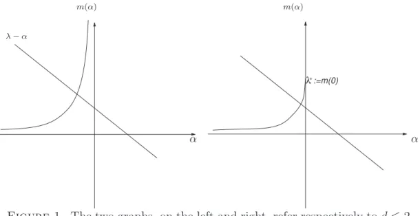
The thermodynamics of the Bose gas (in the free and in the mean field cases) is very well known and does not need to be discussed again here, but its features in terms of loops are not so familiar and, on the other hand, quite interesting and transparent. Recall first that in the free gas there is, in any dimension d ≥ 3, a Bose condensation characterized by the existence of a critical density u∗, so that the free energy
a0(u) := a(u) − u2
2 (3.8)
(i.e. the mean field free energy a(u) minus the mean field energy when the particles density is u) is constant past u∗:
a0(u) = a0(u∗) (3.9)
Such a property is indeed verified by a0(u) as defined by (3.8) with a(u) as in (3.6), which means, recalling (2.4) and (3.7), that, if u ≥ u∗ and [·]
denotes the integer part, lim L→∞ NLlim=[Ldu] N∗ L=[Ldu∗] 1 βLd ln{ ZNL,L ZN∗ L,L } = 0 (3.10)
(3.10) shows that the ratio ZNL,L/ZNL∗,L → 1 (in a very weak sense, indeed).
The closeness to equality before the limit is an indication of validity of the Bose condensation phenomenon in finite volumes. We have a result (proved in appendix B) which shows that the infinite volume description is very accurate:
Theorem 3.1. Let d ≥ 3 and
u∗ = X
j>0
ρ∗j (3.11)
Then, given any density u > u∗ and any two sequences, N
L and NL∗, such
that NL = [Ldu] and NL∗ = [Ldu∗], there is a constant c0, only dependent on
d, such that lim L→∞ ZNL,L ZN∗ L,L = c0 (3.12)
Moreover, there exists another dimension dependent constant c1, such that,
if λ > u∗, lim L→∞ Ξmfλ,Le−βλ2Ld2 Ξmfu∗,Le− β(u∗)2Ld 2 = c1 (3.13)
Let us now describe the condensation phenomenon in terms of loops, starting from the analysis of the functional Fλ(ρ). In any dimension d ≥ 3,
there is a critical chemical potential
λ∗ = X
j>0
ρ∗j = u∗ (3.14)
and, for λ > λ∗, the inf in (3.4) is not a minimum, but (cfr. appendix G) it
is obtained by any minimizing sequence ρ(n) = {ρ(n)
j , j > 0}, such that, for
any fixed j, lim n→∞ρ (n) j = ρ∗j (3.15) while: ρ(λ) := lim n→∞ X j>0 ρ(n)j = X j>0 ρ∗j + (λ − λ∗) = λ (3.16) (3.15)- (3.16) show that a fraction λ−λ∗ of the total mass ρ(λ) concentrates
the r.h.s. of (3.4) has a unique minimizer ρ(λ) = {ρj(λ), j > 0}, where
ρj(λ) = ρ∗jeβjλ0(λ) (3.17)
and λ0(λ) is strictly positive for λ < λ∗, and = 0 otherwise. Thus the total mass of the fluid is
ρ(λ) = X j>0 ρj(λ), if λ ≤ λ∗ X j>0 ρ∗j + (λ − λ∗), if λ ≥ λ∗ (3.18)
and no mass concentrates on infinite loops for λ ≤ λ∗. Note that, by (3.14),
ρ(λ∗) = λ∗.
The validity of the above interpretation follows from following theorem, which is a corollary of the large deviation estimates proved in Appendix E.
Theorem 3.2. For any λ, (3.19), (3.20) and (3.21) below hold.
lim L→∞ P mf λ,L ¡ |jnj Ld − ρj(λ)| > δ ¢ = 0 , ∀δ > 0 (3.19) lim L→∞ P mf λ,L ³ | X j≤J(L) {jnj Ld − ρj(λ)}| > δ ´ = 0 , , ∀δ > 0 (3.20)
independently of the choice of J(L), provided J(L) is an increasing function of L and J(L) ≤ L2. lim L→∞ P mf λ,L ³ |X j≥1 {jnj Ld − ρ(λ)}| > δ ´ = 0 , ∀δ > 0 (3.21)
While the statements relative to global quantities, like pressure, free energy and total number of particles are known in the literature, the results on the way the mass distributes among the different loops are new for the
mean field interaction; Suto, [13], has analogous results in the context of the canonical free measure.
But all this is not really in the focus of our study, which is rather aimed at relaxing the assumption of mean field, for instance considering Kac po-tentials, with the hope that the loops language may provide some simpli-fication. In this perspective it is important to derive sharp estimates on the deviations of the densities in (3.19), (3.20) and (3.21), which have been used in [9] to prove the occurrence of Bose condensation with Kac poten-tials in suitable scaling limits and to get non trivial estimates for the low momenta distribution in the condensed region for a class of long but finite range potential. Results and proofs can be found in Section 5 and Appendix B.
The rate functions of the large deviations of the above macroscopic quan-tities are faithfully described by the functional Fλ(ρ), whose suitably
con-strained minima give the correct large deviations rate functions. Thus, like in the case of the thermodynamical potentials, the analysis of the functional
Fλ(ρ) gives the right answer.
The functional Fλ(ρ) is instead inadequate for studying how the mass of
the condensed fluid (in the Bose condensation regime λ > λ∗) distributes
among the long loops. The issue is discussed in the next section.
4. Distribution of long loops
To study the Bose condensation phenomenon, we restrict to d ≥ 3 and to λ > λ∗. Then, see (3.18)–(3.21) and (3.14), the total mass (after the
fluid” and (λ − λ∗) of the condensed one. By (3.20), lim L→∞ P mf λ,L ³ | X j≤L2 jnj Ld − u ∗| > δ´ = 0 , ∀δ > 0 (4.1)
which shows that in finite volumes the mass of the normal fluid is essen-tially carried by loops with length ≤ L2, while the mass of the condensed concentrates on loops of length > L2:
lim L→∞ P mf λ,L ³ |X j>L2 jnj Ld − (λ − λ ∗)| > δ´ = 0 , ∀δ > 0 (4.2)
Actually most of the mass is on loops whose length is a fraction of the whole volume: lim L→∞ E mf λ,L ³ 1 Ld δLd X j>L2 jnj ´ = δ (4.3)
Furthermore the number ˜XL of loops larger than L2 goes like ln L and
becomes deterministic in the limit L → ∞ (i.e. ˜XL/ ln L → a > 0), while
the cardinality of the subset of loops larger than δLd, δ > 0, is finite and
has a non trivial (i.e. non deterministic) limit distribution.
We summarize this result in the following Theorem proved in Appendix F, where we use the following notation:
yδ,L ≡ 1 Ld X j≥δLd jnj , Xδ,L ≡ X j≥δLd nj , XL ≡ 1 log L X j≥L2 nj (4.4) jmax := max{j : nj > 0}
Theorem 4.1. Suppose that λ > λ∗ and 0 < δ < λ − λ∗, then
lim L→∞E mf λ,L ¡ yδ,L ¢ = λ − λ∗ − δ (4.5) lim L→∞{E mf λ,L ¡ yδ,L2 ¢− Eλ,Lmf¡yδ,L ¢2 } = 1 2δ 2 (4.6)
lim L→∞E mf λ,L ¡ Xδ,L ¢ = log λ − λ∗ δ , L→∞lim E mf λ,L ¡ XL ¢ = d − 2 (4.7) lim L→∞ np log L h Eλ,Lmf¡XL2¢− Eλ,Lmf¡XL ¢2 io = d − 2 (4.8) limL→∞ n Eλ,Lmf¡X2 δ,L ¢ − Eλ,Lmf¡Xδ,L ¢2o = = Dδ = log λ − λ∗ λ − λ∗ − δ µ 1 − logλ − λ ∗ δ ¶ + + Z λ−λ∗−δ δ dx x µ 1 − log λ − λ ∗ λ − λ∗ − x ¶ (4.9) Dδ log[(λ − λ∗)/δ] −−→δ→0 1 (4.10)
Furthermore, for any ξ ∈ (1/2, 1],
lim L→∞P mf λ,L µ jmax Ld > ξ(λ − λ ∗) ¶ = − ln ξ (4.11)
Suto, [13], has already a proof of (4.3) in the free canonical case, but he has not analyzed in detail the statistics of long loops.
5. Small and large deviations 5.1. Small deviations.
Theorem 5.1 (small fluctuations for N ). Let
σ2 := lim L→∞ 1 LdE mf λ,L ¡£ X j>0 j(nj − hnji) ¤2¢ , hnji := Eλ,Lmf(nj) (5.1)
Then, if λ0(λ) is defined as in Appendix G,
σ2 = " β + P 1{λ<λ∗} j ρ∗jjeλ0(λ)βj #−1 (5.2)
for any λ, if d = 3, 4, and for λ 6= λ∗, if d ≥ 5. Moreover, under the same
conditions on λ, the function =(v) := inf
ρ:Pρj=ρ(λ)+v
Fλ(ρ) − inf
ρ Fλ(ρ) (5.3)
with ρ(λ) given by (3.18), is twice differentiable in v = 0 and σ2 = µ β · d2=(v) dv2 ¸ v=0 ¶−1 (5.4)
Proof. The value of σ2 is calculated in Appendix C, Theorem C.2, in
the case λ ≥ λ∗; the case λ < λ∗ could be treated in a similar (simpler)
way. The relation with the free energy functional, equation (5.4), follows
from (I.6) of Appendix I. ¤
Remark: If d = 3 and λ 6= λ∗, equation (5.2) was already obtained by
[2], but the case λ = λ∗ seems new. To check that the expression given
in [2] coincides with (5.2) for λ 6= λ∗, it is sufficient to note that, since
ρ(λ) = λ − λ0(λ) and, in d = 3, ρ∗j = (2πβj)1 3/2 X j ρ∗jβjeλ0(λ)βj = β (2πβ)3/2 X j 1 j1/2e (λ−ρ(λ))βj ≡ β (2πβ)3/2 g1/2 ¡ λ − ρ(λ)¢ (5.5) where g1/2 ¡ µ) is defined in formulas 17-18 of [2].
We will also study deviations of other macroscopic quantities. In partic-ular we will consider the following sets:
V1 := Z+ V2 := {`} V3 := {J(L)} V4 := {1, 2, . . . , J(L)} (5.6) with J(L) as in Theorem 3.2, namely J(L) ∈ N+ is an increasing function of L, such that lim
L→∞J(L) = ∞ and limL→∞J(L)/L
For k = 1, .., 4, we then define A(k)L,δ(v) ≡ A(k)L,δ := ( n : 1 LdN (k) ∈ Ã X j∈Vk ρj(λ) + v − δ, X j∈Vk ρj(λ) + v + δ !) (5.7) A(k)L (v) ≡ A(k)L := ( ρ : X j∈Vk ρj = X j∈Vk ρj(λ) + v ) (5.8) with N(k) = X j∈Vk jnj (5.9) and ρj(λ) as in (3.17).
The small deviations for N(k), k 6= 1, N(k) as in (5.9), are discussed in Appendix D for λ > λ∗. The relation of the corresponding covariances with
the free energy functional goes along the same lines of Appendix I and we omit it.
5.2. Large deviations.
In this subsection we will express the rate functions of large deviations for the quantities (5.7), (5.8) in terms of variational problems for the limit functional with corresponding constraints.
Theorem 5.2. For any λ, if k = 1, and for any λ 6= λ∗, if k > 1,
lim δ→0 L→∞lim 1 βLd ln P mf λ,L ³ A(k)L,δ ´ − inf ρ∈A(k)L Fλ(ρ) + inf ρ Fλ(ρ) = 1 (5.10)
Proof. The proof of this Theorem in the case k = 4 and λ > λ∗ (the
most interesting case) follows from Theorem E.3 in Appendix E and Ap-pendix H. The other cases can be treated along the same lines. ¤
Remark: The case λ = λ∗ is more involved, if k > 1, so we did not
study it in detail, but we think that Theorem 5.2 is still valid.
Corollary 5.3 (large deviations for N(1) ≡ N).
lim δ→0L→∞lim ln P (A(1)L,δ) βLd = −¯t(ρ(λ) + v) + v2 2 + ρ(λ)v + π 0 λ0(λ+¯t) − π 0 λ0(λ) (5.11)
where λ0(λ) is defined in (G.5), πλ00 is the pressure of the free system with
chemical potential λ0 (cfr. equation (G.2)) and ¯t is the solution of the
equation ¯t = λ0(λ + ¯t) − λ0(λ) + v.
Remark: If λ > λ∗ and λ + v > λ∗, then ρ(λ) = λ, λ
0 = 0 and the expression on the r.h.s. of (5.11) becomes −v2
2 .
Corollary 5.4 (large fluctuations for N(2) and N(3)). If λ ≥ λ∗, −ρ∗` < v < λ − λ∗ and we define θ := v ρ∗ `, then lim δ→0L→∞lim 1 βLd ln P (A (2) L,δ) = − 1 β v ` £ (θ−1+ 1) ln (1 + θ) − 1¤ (5.12) while, if λ ≥ λ∗ and v > λ − λ∗, lim δ→0L→∞lim 1 βLd ln P (A (2) L,δ) (5.13) = −1 β v ` £ (θ−1+ 1) ln (1 + θ) − 1¤+ λ20 2 − λ0 + π 0 λ0 − π 0 0 where λ0 = λ0(λ − ρ∗` − v). If λ > λ∗ and v > 0: lim δ→0L→∞lim J(L) βLdln J(L)ln P (A (3) L,δ) = − vd 2 (5.14)
For λ > λ∗ and v < 0 we get:
lim δ→0L→∞lim 1 βLdln P (A (3) L,δ) = − c(v)d 2 (5.15)
Proof. By Theorem 5.2 and Appendix H lim δ→0L→∞lim 1 βLd ln P (A (2) L,δ) = −¯t(ρ`(λ) + v) + πλ,¯t− πλ (5.16)
where ¯t is the solution of the equation ρ`(λ)e¯tβ` = ρ`(λ) + v. The solution
does exist when v > −ρ`(λ) and is given by:
¯t = 1 β`ln µ ρ`(λ) + v ρ`(λ) ¶ (5.17) When λ > λ∗ and −ρ∗` < v < λ − λ∗, we see that ˜πλ,¯t− πλ = λ
2 2 + 1 β P j (ρ∗ j+v1j=`) j − λ 2 2 − β1 P j ρ∗ j j = β`v , so that, defining θ := ρv∗ `, lim δ→0L→∞lim 1 βLd ln P (A (2) L,δ) = − 1 β v ` £ (θ−1+ 1) ln (1 + θ) − 1¤ (5.18) while, if v > λ−λ∗, we get an extra term coming from the difference ˜π
λ,¯t−πλ.
(5.14) is a direct consequence of (5.12), obtained in the limit θ → ∞. ¤
Notice that, when λ > λ∗, in the limit L → ∞, the fluctuation of ρ ` has
the law of a free Poisson distribution with parameter ρ∗ `.
Corollary 5.5 (large deviations for N(4) ). For λ > λ∗; v > 0:
lim δ→0L→∞lim J(L) βLdln J(L)ln P (A (4) L,δ) = −v µ d 2 − 1 ¶ (5.19)
For v < 0 and all λ ≥ λ∗, we have instead,
lim sup L→∞ 1 Ld log P mf λ,L ³Xj(L) j=1 jnj ≤ [u∗ − |v|]Ld ´ ≤ −c(v) (5.20)
where c(v) > 0 and vanishes as v → 0 as c(v) ∼ v2 d ≥ 5 v2 | log |v|| d = 4 |v|3 d = 3 (5.21)
Proof. See Theorem E.3 and Appendix H ¤
6. Long loops and Bose condensation.
In this section we show that, in the mean field model, the excess density concentration ρ − ρ∗ on large loops implies the phenomenon of condensation
(i.e. a finite fraction of the number of particles occupies the state of zero momentum ).
The reduced density matrices (RDM) are the quantum analogue of cor-relation functions [1] [12] and the Fourier transform of the one point RDM, in the case of periodic boundary conditions with translational invariant po-tentials, gives (Onsager Penrose [11]) the average number of particles of momentum 2πp/L, p ∈ Zd: ˆ ρΛ(p) = Z Λ ρΛ(0, z)ei 2πp L z dz (6.1)
Using the language of loops, in the mean field case, where the interaction does not depend on the position of the particles, the one point RDM reads [5]: ρmfΛ (x, y) = X j0 Ξ−1λ,LX n w(n)e−β( P j j(nj +δj,j0 ))2 2Ld eλβj0 X k∈Zd e−(kL+(x−y))22βj0 (2πβj0)d/2 (6.2)
Theorem 6.1. For d ≥ 3 and any β, when λ is larger than λ∗ lim L→∞ ˆ ρmfΛ (0) Ld = λ − λ ∗ (6.3)
Proof From (6.1) and (6.2) we get that: ˆ ρmfΛ (0) = Z Λ ρmfΛ (0, z) dz = X j0 Ξ−1λ,LX n w(n)e−β( P j j(nj +δj,j0 ))2 2Ld eλβ P jj(nj+δj,j0) = Eλ,Lmf à X j jnj Lda(βj, L) ! (6.4) The Theorem is proved using (4.5) and (cfr. (D.62))
0 < a(βj, L) − ρj ≤ Cρje−L
2/(2βj)
¤
Appendix A
In this appendix we recall the relation between the usual definition of the canonical partition function for a free Bose gas and its representation in the loops language given in (2.4).
The canonical partition function for a system of N identical bosons is
ZN = Tr e−βHN
where HN is the Hamiltonian operator and the trace involves only
Theorem A.1. Let HN = − N
X
i=1
∆i be the hamiltonian of N free Bosons
in a cubic box of size L with periodic boundary conditions, then ZN,L = X ν:|ν|=N e−βPp(2πpL ) 2 νp = X n:Pjnj=N Y j 1 nj! P pe−βj( 2πp L ) 2 j nj (A.1)
Proof. The Bosons states in the momentum representation can be
writ-ten as |ν >= |νp , p ∈ Zd >, νp being the number of Bosons with
momen-tum equal to k = 2πpL−1. The energy in such a state is equal to Pp²pνp,
²p =
¡
2πpL−1¢2, hence the first equality in (A.1).
To prove the second one, let λ < 0 and define:
Z(λ) := X
N
eβλN X
ν:|ν|=N
e−βPp²pνp (A.2)
that can be rewritten as:
Z(λ) = exp ( −X p ln(1 − e−β(²p−λ)) ) = exp ( X j à X p e−β(²p−λ)j j !) = X M 1 M ! " X j à X p e−β(²p−λ)j j !#M = X n Y j " X p e−β(²p−λ)j j #nj 1 nj! (A.3) = X N eβλN X n:Pjjnj=N Y j "P pe−βj²p j #nj 1 nj!
Since Z(λ) is analytic in λ for Re λ < 0, (A.1) follows.
An alternative proof working in the configuration representation can be obtained as follows. ZN,L = 1 N! X π Z dr1. . . drNhrπ1. . . rπN|e −βHN|r 1. . . rNi
where Pπ is the sum over all permutations of (1, 2, . . . , N ). Since any permutation breaks up into cycles (loops), we have
ZN = 1 N ! X n1,n2,... c(n1, n2, . . . ) Y j Znj where a) c(n1, n2, . . . ) = N! Y j 1 jnj 1
nj! is the number of ways of having n1 loops
of length 1, n2 of length 2, etc.
b) the sum is over all combinations of permutations s.t. Pjnj = N
c) Z(j) = X
p
e−βj²p, where −²
p are the eigenvalues of the Laplace
oper-ator ∆.
In the case of a free Bose gas in a cubic box of size L with periodic boundary conditions ZN,L = X n:Pjnj=N Y j 1 nj! P pe−βj( 2πp L ) 2 j nj
thus deriving again the last equality in (A.1).
Finally, to justify equation (2.3), we prove the following lemma.
Lemma A.2. For any L and α > 0
Ld X k∈Zd e−(kL)2/(2α) (2πα)d/2 = X k∈Zd e−12α(2πk/L)2 (A.4)
Proof. Equation (A.4) follows from the identities e−(kL)2/(2α) = 1 (2π)d/2 Z Rd e−x2/2+iLkx/√αdx (A.5) and 1 (2π)d X k∈Zd eivk = X k∈Zd δ(v − 2πk) (A.6) ¤ Appendix B
The canonical partition function (A.1) of the free Bose gas can be written as ZN,L = X {nk}
1
P nk=N e −βPknkEk = N X M =0 ˜ ZM,L (B.1) ˜ ZM,L = X {nk,k6=0}1
P k6=0nk=M e −βPk6=0nkEk (B.2)where the momentum k takes values in the set {2πn/L, n ∈ Zd}, n
k ∈ Z
and Ek = k2/2.
In this appendix we study the tail properties of the probability distribu-tion on N with density
PL(M ) = ˜ ZM,L QL , QL = ∞ X M =0 ˜ ZM,L (B.3)
and mean value
< M >L= X k6=0 1 eβEk − 1 ≡ L dλ∗ L (B.4)
We remark that this probability distribution is the canonical distribution of the total number of particles with k 6= 0 for a free Bose gas. These results
will be used in the sequel to prove small and large deviation both in the free and mean field case.
We want to study the asymptotic properties of the probability measure PL
as L → ∞. To begin with, note that, if d ≥ 3, limL→∞λ∗L does exist and
λ∗ = lim L→∞λ ∗ L = Z Rd dk (2π)d 1 eβEk − 1 (B.5) Let us define cL = Ld−2(λ∗ − λ∗L) (B.6)
Lemma B.1. For any d ≥ 3, cL has a limit as L → ∞ and
c∗ ≡ lim L→∞cL = Z ∞ 0 dt 1 −X n6=0 e−n2/(2βt) (2πβt)d/2 (B.7)
Proof. (3.2) and (B.4) imply that
Ldλ∗L = X k6=0 ∞ X j=1 e−βjEk = ∞ X j=1 £ Lda(βj, L) − 1¤ (B.8) while (B.5) implies that
Ldλ∗ = Ld ∞ X j=1 1 (2πβj)d/2 (B.9)
hence, by using the definition of a(t, L) in (3.2), we get
cL = 1 L2 ∞ X j=1 1 − X n6=0 e−n2/(2βtj) (2πβtj)d/2 , tj = j L2 (B.10)
The lemma follows from this expression, easily implying the convergence of the sum over j ≤ L2, and the identity, following from (3.2) (with L = 1),
1 −X n6=0 e−n2/(2t) (2πt)d/2 = 1 (2πt)d/2 − X n6=0 e−2π2tn2 (B.11)
which implies immediately the convergence of the sum over j ≥ L2. ¤ Let us now define
yL = M − L dλ∗ L hL , hL = L2 d = 3 L2√log L d = 4 Ld/2 d ≥ 5 (B.12) An important role in this appendix has the following Theorem
Theorem B.2. If M is a random variable with probability (B.3), the
distribution function of the random variable yL converges, as L → ∞,
to the distribution function of a random variable y on R with mean 0 and smooth density ρ(y) strictly positive, whose Laplace transform F (σ) =
R
dyρ(y) exp(−σy), σ ∈ C, is given, if d = 3 and <σ > −2π2β, by
F (σ) = exp X n6=0 G µ σ 2π2βn2 ¶ , G(u) = u − log(1 + u) (B.13) while, if d ≥ 4 and <σ ∈ R, F (σ) = e12c0σ2 , c0 = ( 1 2π2β2 d = 4 1 (2πβ)d/2 P∞ j=1j1−d/2 d ≥ 5 (B.14)
Moreover, there exists a constant C, independent of L and M, such that
(1 + yL2)hLPL(M) ≤ C (B.15)
and, given any y ∈ R, if we choose M = ML∗ so that yL∗ = (ML∗ − Ldλ∗
L)/hL −−−→L→∞ y, then
hLPL(ML∗) −−−→L→∞ ρ(y) (B.16)
Proof. To begin with, we shall prove that the Laplace transform of
yL, FL(σ) =
P∞
M =0PL(M) exp[−σ(M − Ldλ∗L)/hL], is well defined and
σ0 = −∞, if d ≥ 4; this implies in particular that the characteristic func-tion fL(t) = FL(−it), t ∈ R, is convergent for any t. By analyzing the
decaying properties in t of fL(t), we shall also prove the bound (B.15),
im-plying that the distribution function of yL is convergent and that its limit is
the distribution function of a probability measure on R; in fact, by a simple application of dominated convergence Theorem,
X 0≤M ≤hLy+Ldλ∗L PL(M ) = 1 hL X 0≤M ≤hLy+Ldλ∗L hLPL(M ) −−−→L→∞ Z y −∞ ρ(z)dz (B.17) Note that this result follows from the convergence of fL(t) to f (t), without
using the bound (B.15), since PL(M ) is a probability measure [3]. We
are stressing here the role of (B.15) only because we shall generalize in the following the previous argument to some cases where PL(M) is not a
probability measure, even if P∞M =0PL(M) = 1.
Finally, by analyzing the properties of the limiting measure Laplace transform, we shall prove that this measure has a smooth and strictly pos-itive density.
By a straightforward calculation, one can see that log FL(σ) = L dλ∗ L hL σ −X k6=0 log1 − e−βEk−σ/hL 1 − e−βEk = = X k6=0 · σ hL 1 eβEk − 1 − log µ 1 + 1 − e −σ/hL eβEk − 1 ¶¸ = (B.18) = X k6=0 1 eβEk − 1 · σ hL − (1 − e −σ/hL) ¸ +X n6=0 G µ 1 − e−σ/hL e2π2βn2/L2 − 1 
where G(u) = u − log(1 + u).
Let us consider first the case d = 3. Then hL = L2, so that FL(σ) is well
defined for <σ > σ0 ≡ −2π2β; hence we shall fix σ so that this condition is satisfied. Then the first term in the third line of (B.18) goes to 0 as L → ∞,
since it is bounded by CL−1, where C (here and in the following) denotes a
suitable positive constant, depending on σ but independent of L. Note that
un,L ≡ 1 − e −σ/hL e2π2βn2/L2 − 1 −−−→L→∞ u ∗ n ≡ σ 2π2βn2 (B.19)
and that |un,L|, |u∗n| ≤ Cn−2 and |un,L − u∗n| ≤ C/L2. On the other hand,
<un,L and <u∗n are larger of some constant u0 > −1, for any n; since G0(u) =
u/(1 + u), it immediately follows that
|G(un,L) − G(u∗n)| ≤ C|un,L − u∗n|n−2 ≤ Cn−7/2|un,L − u∗n|1/4 ≤
≤ C|n|−7/2L−1/2 (B.20)
It follows that log FL(σ) and FL(σ) are convergent for L → ∞ and that, if
F (σ) = limL→∞FL(σ), Π(σ) ≡ log F (σ) = X n6=0 G µ σ 2π2βn2 ¶ (B.21) It is not hard to show that Π(σ) is differentiable and that
Π0(σ) = X n6=0 σ 2π2βn2(σ + 2π2βn2) (B.22) implying that, if x ∈ R, lim x→+∞Π 0(x) = +∞ , lim x→σ+0 Π0(x) = −∞ (B.23)
Let us now call P (dy) the probability measure such that
F (σ) = eΠ(σ) = Z
P (dy) e−σy (B.24) The property (B.23) easily implies that the support of P (dx) is the full real line. Moreover, the characteristic function f (t) of P (dx) is given by the equation f (t) = eΠ(−it) = Y n6=0 e−itan−2 1 − itan−2 , a = (2π 2β)−1 (B.25)
By using the bound log(1 + x) ≥ 2x/3, valid for 0 ≤ x ≤ 1/2, we get, if |t| ≥ 1, |f (t)| ≤ Y n6=0 (1 + t2a2|n|−4)−1/2 ≤ ≤ Y |n|≤(√2a|t|)1/2 (3/2)−1/2 Y |n|>(√2a|t|)1/2 e−t2a2|n|−4/3 ≤ e−C|t|3/2 (B.26) This bound and the support properties of P (dy) imply that P (dy) = ρ(y)dy, with ρ(y) a strictly positive smooth function on R.
In order to complete the proof of the Theorem in the case d = 3, we still have to prove the strong convergence property (B.16), together with the uni-form bound (B.15) on hLPL(M ). Note that the definition of characteristic
function implies that
hLPL(M) = 1 2π Z +πhL −πhL dt e−ityLf L(t) (B.27)
By using (B.18), we see that
fL(t) = FL(−it) =
Y
n6=0
evn,L
1 + un,L (B.28)
where un,L is given by (B.19) with σ = −it and
vn,L = −it L2(e2π2βn2/L2 − 1) (B.29) It follows that |fL(t)| ≤ Q
n6=0|1+un,L|−1. Moreover, by using (B.19), we see
that, if |t| ≤ πL2/2 and |n|2 ≤ |t|, |1 + u n,L| ≥ 1 + δ, with a suitable δ > 0. Hence, if |t| ≤ πL2/2, |f L(t)| ≤ Q 0<|n|≤|t|1/2(1 + δ)−1 ≤ exp(−C|t|−3/2). If
πL2/2 ≤ |t| ≤ πL2, the same result is obtained, by observing that in this case, if |n| ≤ L, |1+un,L| ≥ 1+1/(e2π
2β
−1), so that |fL(t)| ≤ exp(−CL3) ≤
exp(−C|t|−3/2). Hence, we can show that, uniformly in L,
which implies, together with (B.27), that hLPL(M) ≤ C, with C
inde-pendent of L and M . Moreover, by the dominated Lebesgue convergence Theorem, we get, for any y ∈ R,
yL −−−→L→∞ y ⇒ hLPL(M ) −−−→L→∞ 1
2π
Z +∞
−∞
eityf (t) = ρ(y) (B.31) In order to complete the proof of (B.15), we use the identity
(−iyL)2hLPL(M) = 1 2π Z +πhL −πhL e−ityLf00 L(t) (B.32)
Since fL00(t) = fL(t)[Π0L(−it)2 + Π00L(−it)], where ΠL(−it) = log FL(−it),
and, as one can check easily by proceeding as in the analysis given before of log FL(σ), uniformly in L,
|Π0L(−it)| ≤ C|t| , |ΠL(−it)| ≤ C (B.33)
the bound (B.15) immediately follows from the bound (B.30). Let us now suppose that d = 4. Then hL = L2
√
log L, so that, given any
x < 0, FL(σ) is well defined for <σ > x, if L > exp(−x/(2π2β). Moreover,
as in the case d = 3, the first term in the third line of (B.18) goes to 0 as
L → ∞, since it is bounded by C(log L)−1/2.
If we define un,L as in (B.19), |un,L| ≤ C(n2
√
log L)−1, with C only
depending on σ if L is large enough. Hence, if ˜G(u) = u − log(1 + u) − u2/2, ¯ ¯ ¯ ¯ ¯ ¯ X n6=0 ˜ G(un,L) ¯ ¯ ¯ ¯ ¯ ¯ ≤ C (log L)3/2 X n6=0 1 |n|6 −−−→L→∞ 0 (B.34)
Note also that L−4P
|n|≥L[exp(an2/L2) − 1]−2 is bounded for L → ∞, for
any a > 0, and that 1 log L X 0<|n|≤L · 1 (an2)2 − 1 L4(ean2/L2 − 1)2 ¸ ≤ C L2log L X 0<|n|≤L 1 |n|4 −−−→L→∞ 0 (B.35) so that (log L)−1L−4P
n6=0[exp(an2/L2) − 1]−2 is convergent for L → ∞ and
c0 = lim L→∞ 1 log L X n6=0 1 L4(ean2/L2 − 1)2 = limL→∞ 1 log L X 0<|n|≤L 1 a2|n|4 = = 1 a2 L→∞lim 1 log L Z 1≤|x|≤L d4x |x|4 = 2π2 a2 (B.36)
Bu using (B.18) and (B.36) with a = 2π2β, it is now easy to prove that
log FL(σ) is convergent for L → ∞ and that
Π(σ) = lim L→∞log FL(σ) = (B.37) = 1 2σ 2 lim L→∞ 1 L4log L X n6=0 1 (e2π2βn2/L2 − 1)2 = 1 2 2 (2πβ)2σ 2
It follows immediately, if we define P (dy) as in the case d = 3, that P (dy) is a Gaussian probability measure with density ρ(y) = (2πc0)−1/2exp[−y2/(2c0)], with c0 = 2/(2πβ)2. The proof of (B.15) and (B.16) in the case d = 3 can be easily extended to this case; we omit the details.
Let us finally consider the case d ≥ 5. Then hL = Ld/2 and we can
proceed as in the previous case, the only relevant difference being that now Π(σ) gets a contribution also from the first term in the third line of (B.18).
We find that Π(σ) = 12c0σ2, with c0 = lim L→∞ 1 Ld X n6=0 · 1 e2π2βn2/L2 − 1 + 1 (e2π2βn2/L2 − 1)2 ¸ = (B.38) Z ddk (2π)d e−βEk (1 − e−βEk)2 = X j1,j2≥0 Z ddk (2π)de −βEk(j1+j2+1) = X j≥1 j (2πβj)d/2
The proof of (B.15) and (B.16) in the case d = 3 can be easily extended also to this case, so completing the proof of the Theorem. ¤
Appendix C. Proof of Theorem 3.1
Note that the mean field grand canonical partition function can be writ-ten as Ξmfλ,L = e12βλ2Ld ∞ X N =0 e−β2Ld(LdN−λ) 2 ZN,L (C.1) and that PL(M ≤ N ) = PL µ yL ≤ L d hL(λ − λ ∗) + Ld/2 hL xN + L2 hLcL ¶ (C.2) xN = Ld/2(N Ld − λ)
Let us now define Γλ,L ≡ Ξmfλ,L e12βλ2LdQLLd/2 = 1 Ld/2 ∞ X N =0 e−β2Ld(LdN −λ) 2 PL(M ≤ N ) (C.3)
Lemma C.1. If λ ≥ λ∗, the quantity Γ
λ,L has a limit as L → ∞. If
λ > λ∗, we have, for any d ≥ 3,
lim L→∞Γλ,L = r 2π β (C.4) while, if λ = λ∗, we have 0 < lim L→∞Γλ,L = q 2π β Rc∗ −∞dyρ(y) d = 3 q π 2β d = 4 R+∞ −∞ dxe−βx 2/2Rx −∞dyρ(y) d ≥ 5 (C.5)
where ρ(y) is the density probability defined in Theorem B.2.
Moreover, if NL = [uLd] ([·] denotes the integer part), u > λ∗, and
NL∗ = [λ∗Ld], then lim L→∞ ZNL,L ZN∗ L,L = ( 1/P (y ≤ c∗) d = 3 2 d ≥ 4 (C.6) Proof. By theorem B.2, PL(yL ≤ ¯y) −−−→L→∞ Ry¯
0 dyρ(y), for any fixed ¯
y, ρ(y) being a strictly positive function depending on the dimension d.
Hence, by using (C.2) and Lemma B.1, we can easily show that, if λ > λ∗ and xN −−−→L→∞ x, PL(M ≤ N) −−−→L→∞ 1 , ∀x (C.7) while, if λ = λ∗ and x N −−−→L→∞ x, PL(M ≤ N) −−−→L→∞ P (y ≤ c∗) d = 3 P (y ≤ 0) = 1/2 d = 4 P (y ≤ x) d ≥ 5 (C.8)
Then (C.4) and (C.5) follow from (C.3) and a simple application of the dominated Lebesgue convergence theorem. The proof of (C.6) is a simple
consequence of (C.2), (C.8) and the equation, valid if NL = [uLd], u > λ∗, and NL∗ = [λ∗Ld], lim L→∞ ZNL,L ZN∗ L,L = lim L→∞ PL(M ≤ NL) PL(M ≤ NL∗) = lim L→∞ PL(yL ≤ L d hL(u − λ ∗)) PL(yL ≤ cLL2/hL) (C.9) ¤ By similar arguments, one can prove the following Theorem (see also [2] for the case λ > λ∗).
Theorem C.2. If λ > λ∗, the distribution of the random variable x N
converges, as L → ∞, to a Gaussian distribution with density exp(−βx2/2); the same result is true if λ = λ∗ and d = 3, 4. However, if d > 4, the
limiting distribution is still well defined, but it is not Gaussian anymore; it is proportional to e−βx2/2Rx
−∞dyρ(y), ρ(y) being the density probability
defined in Theorem B.2.
Appendix D. Distribution of “short loops”
In this appendix we will restrict to d ≥ 3 and λ ≥ λ∗ and study the
distribution of the variables
yA,L = P j∈Ajnj − LdρA,L hA,L , ρA,L = X j∈A ρj,L (D.1)
where A is a finite subset of N+, LDρj,L is the mean value of jnj with respect
to the mean field measure and hA,L is a suitable scaling factor. The main
results are stated in Theorems D.4 and D.5 below, the main ingredient in the proofs is the reduction to the analysis of the probability distribution
We start by deriving the following expression for ρj,L: ρj,L = a(βj, L) αj,L (D.2) where αj,L = 1 Γλ,L 1 Ld/2 X N ≥0 e−βx2N/2P L(M ≤ N − j) (D.3) with xN as in (C.2). Proof of (D.2) - Let w0(j, n j) be as in (2.1) with λ = 0, then: ρj∗,L = e βλ2 2 Ld Ξmfλ,L X N e−βx2N2 X n:Pjjnj=N Y j w0(j, nj) j∗n j∗ Ld = e βλ2 2 Ld Ξmfλ,L a(βj ∗, L)X N e−βx22NZN −j∗,L (D.4) By (B.1) and (B.3) we get: ρj∗,L = e βλ2 2 Ld Ξmfλ,L a(βj ∗, L)Q L X N e−βx2N2 PL(M < N − j∗) (D.5) hence (D.2) follows by (C.3). ¤
Lemma D.1. For any λ ≥ λ∗, there is a constant C, independent of L
and j, such that, if hL is defined as in (B.12),
0 < 1 − αj,L ≤ C j hL (D.6) Moreover, if λ = λ∗, lim L→∞ hL j (1 − αj,L) = ρ(c∗) Rc∗ −∞dyρ(y) d = 3 2ρ(0) d = 4 R+∞ −∞ dxe−βx2/2ρ(x) R+∞ −∞ dxe−βx2/2 Rx −∞dyρ(y) d ≥ 5 (D.7)
Proof. Note that 1 − αj,L = 1 Γλ,L 1 Ld/2 X N ≥0 e−βx2N/2P L(N − j < M ≤ N) (D.8)
By using the claim in Lemma C.1 that hLPL(M) is bounded uniformly in
L and M , we get PL(N − j < M ≤ N) = 1 hL N X M =N −j+1 hLPL(M ) ≤ C j hL (D.9)
which immediately implies (D.6), by using Lemma C.1. On the other hand, if λ = λ∗ and M = N − r, r ≥ 1, the corresponding y
L variable is equal, see
(C.2), to (Ld/2x N + L2cL− r)/hL, so that, by using (B.16), hLPL(M = N − r) −−−→L→∞ ρ(c∗) d = 3 ρ(0) d = 4 ρ(x) d ≥ 5 (D.10)
(D.7) then follows from Lemma C.1 and dominated convergence Theorem. ¤ If λ > λ∗, h
LPL(M = N −r) goes to 0 as L → ∞, so we expect the bound
(D.6) can be improved. This is especially true if j is taken as a diverging function of L; in particular, if j > (λ − λ∗)Ld, it is easy to see that α
j,L → 0
as L → ∞. In order to get good bounds in all these cases, we shall use the following large deviation bound for the probability measure PL(M ).
Lemma D.2. Let 0 < u1 < u2; then there exist ¯L(u1), such that the
probabilities
SL+(u1, u2) ≡ PL(Ldλ∗L+ Ldu1 ≤ M ≤ Ldλ∗L+ Ldu2) (D.11)
satisfy, for L ≥ ¯L(u1), the following bounds. e−a1u2Ld−2(1+δL) ≤ S+ L(u1, u2) ≤ e−a1u1L d−2(1−δ L) , ∀u 1 > 0 (D.13) e−f (u2)(Ld/hL)2(1+δL) ≤ S− L(u1, u2) ≤ e−f (u1)(L d/h L)2(1−δL) , u 2 < λ∗ (D.14)
where δL is a function which goes to 0 as L → ∞, a1 is a positive constant,
depending on d, and f (u) is a positive function of order u2 for u → 0 (equal indeed to a2u2 for d = 2, 3).
Proof. By (C.2), we can write
SL+(u1, u2) = Z u2Ld/h L u1Ld/hL PL(dy) = eΠL(t) Z u2Ld/h L u1Ld/hL etyPt,L(dy) (D.15)
where ΠL(t) = log FL(t), FL(t) is the Laplace transform of PL(dy) given by
(B.18), t is any real number such that FL(t) is well defined and Pt,L(dy) is
the probability measure
Pt,L(dy) = e −tyP
L(dy)
FL(t)
(D.16) By looking at (B.18), we see that FL(t) is defined for t > t∗L, where t∗L is the
value of t such that the argument un,L of the function G(u) = u − log(1 + u)
is equal to −1 if |n| = 1, that is t∗
L = −ahL/L2. We choose t so that
−Π0L(t) = Z dy y Pt,L(dy) = vL d hL , v = u1 + u2 2 (D.17)
By using (B.18), this condition can be written 1 hL X n6=0 (e−t/hL − 1)ean2/L2 (ean2/L2 − e−t/hL)(ean2/L2 − 1) = v Ld hL , a = 2π 2β (D.18)
By proceeding as in the proof of Theorem B.2, it is easy to see that the sum in the l.h.s. is bounded by C|t|, if we extract from it the terms with
|n| = 1; hence we get cL− d t h2 L 1 a/L2 + t/h L L2 a (1 + δ1,L) = v Ld hL (D.19)
with δ1,L → 0 and cL → c as L → ∞. It follows that
tL
d
hL
= −aLd−2(1 + δ2,L) (D.20)
with δ2,L → 0 as L → ∞. It is easy to see that, for such a value of t, ΠL(t)
diverges as C log L for d = 3, 4 and as Ld−4 for d ≥ 5, so that we can write
SL+(u1, u2) = e−avL d−2(1+δ L) Z u2Ld/h L u1Ld/hL et(y−vLd/hL)P t,L(dy) (D.21)
with δL → 0 as L → ∞. The upper bound in (D.13) easily follows from
this equation. In order to prove the lower bound we have also to show that Z u2Ld/h
L
u1Ld/hL
Pt,L(dy) ≥ 1 − δL (D.22)
with δL → 0. This result can be deduced as the other ones from the
proper-ties of the Laplace transform of the measure Pt,L(dy); we omit the details.
Let us now consider the upper bound of (D.14). We proceed as before, by writing SL−(u1, u2) = eΠL(t)−tΠ 0 L(t) Z −u1Ld/h L −u2Ld/hL et(y+u1Ld/hL)P t,L(dy) ≤ ≤ eΠL(t)−tΠ0L(t) (D.23)
where t is chosen so that Π0
L(t) = u1Ld/hL. It is easy to see that Π0L(t) is
a monotone function and that limt→∞Π0L(t) = λ∗LLd/hL, so that t is well
defined for L large enough, if u1 < λ∗. It turns out that limL→∞t(hL/Ld) =
for some cd > 0). Moreover ΠL(t) − tΠ0L(t) = − Z t 0 ds Z s 0
duΠ00L(u) , C/2 < Π00L(u) ≤ C (D.24) and one can prove that limL→∞Π00l(u) = Cd > 0, uniformly for 0 ≤ u ≤ t;
this allows us to get the upper bound in (D.14). The lower bound is obtained in a similar way, by choosing t so that Π0
L(t) = u2Ld/hL and by proving
that R−u1Ld/hL
−u2Ld/hL Pt,L(dy) → 1/2 for L → ∞. ¤
We can now prove the following bounds on the factors αj,L.
Lemma D.3. Given d ≥ 3, λ > λ∗ and a sequence jL such that
lim
L→∞jL/L
d = γ < (λ − λ∗) (D.25)
there exists ¯L such that, if L ≥ ¯L and j ≤ jL,
1 − αj,L ≤ Ce−a3(λ−λ
∗−γ)Ld−2
(D.26)
where C and a3 are constants independent of L and of j.
Moreover, if λ ≥ λ∗ and γ > λ − λ∗, there exist C, a4 and ¯L such that,
if L ≥ ¯L and j ≥ jL,
αj,L ≤ Ce−a4[γ−[λ−λ
∗)]Ld−1
(D.27)
Proof. Note that
PL(N − j < M ≤ N ) ≤ ≤ PL µ yL ≥ (λ − λ∗)Ld+ c LL2 + xNLd/2 − j hL ¶ (D.28) Hence, if j ≤ jL, with jL/Ld → γ as L → ∞, and |xN| ≤ L(d−1)/2, so that
|xN|Ld/2/hL ≤ L−1/2Ld/hL, PL(N − j < M ≤ N) ≤ PL µ yL ≥ (λ − λ∗ − γ − δ L)Ld hL ¶ (D.29)
with δL → 0 as L → ∞. On the other hand 1 Ld/2 ∞ X N =0 e−β2x2N
1
|xN|≥L(d−1)/2 ≤ Ce −β4Ld−1 (D.30) The bound (D.26) then easily follows from (D.8) and Lemma D.2 since the upper bound in (D.13) is independent of the u2 value (equal to +∞ in this case).The bound (D.27) is proved in a similar way, by using the upper bound in (D.14) and the remark that Ld−1 ≤ (Ld/h
L)2. ¤
We have now all the technical ingredients to study the Laplace transform
FA,L(σ) of the probability distribution of the random variables yA,L defined
in (D.1). We have FA,L(σ) = e σLdρA,LhA,L Γλ,L 1 Ld/2 X N ≥0 e−βx2N/2 1 QL X {nj≥0,j≥1}
1
P jnj=N · · Y j /∈A w(j, nj) Y j∈A w(j, nj)e−σ jnj hA,L (D.31)By using (2.14) and the identity
w(j, n)e−σhA,Ljnj = (D.32) = X {n0,n00≥0}
1
n0+n00=n 1 n0! "Lda(βj, L)e−σhA,Lj − 1
j #n0 1 n00! µ 1 j ¶n00 we see that FA,L(σ) = GA,L(σ) 1 Γλ,L 1 Ld/2 X N ≥0 e−βx2N/2P A,L,σ(M ≤ N ) (D.33)
where PA,L,σ(M) = Q−1A,L,σ X {nj≥0,j≥1}
1
P jnj=M · · Y j /∈A ˜ w(j, nj) Y j∈A ˜ w(j, nj, σ) (D.34) QA,L,σ = X {nj≥0,j≥1} Y j /∈A ˜ w(j, nj) Y j∈A ˜ w(j, nj, σ) (D.35) ˜ w(j, n, σ) = 1 n! "Lda(βj, L)e−σhA,Lj − 1
j #n (D.36) GA,L(σ) = eσ LdρA,L hA,L QA,L,σ QL (D.37) Note that PA,L,σ(M ) in general is not a probability distribution for any value
of σ (this is clear only for σ real and negative). Moreover, in all the choices of the set A we shall consider, PA,L,σ(M ) is absolutely summable over M
and its sum is equal to 1 (which is formally true by definition). Hence, we can consider it as a finite complex measure on R (with support on a lattice set) and we shall study its convergence, as L → ∞, to a measure with smooth density.
A few simple calculations show that log QA,L,σ =
X
j∈A
Lda(βj, L)e−σhA,Lj − 1
j + X j /∈A Lda(βj, L) − 1 j (D.38) so that log GA,L(σ) = σL dρ A,L hA,L +X j∈A Lda(βj, L) j ³ e−σhA,Lj − 1 ´ = = σ rA,L∗ +X j∈A Lda(βj, L) j µ e−σhA,Lj − 1 + σ j hA,L ¶ (D.39)
where rA,L∗ = L d hA,L X j∈A a(βj, L)(αj,L− 1) (D.40)
It will also useful to consider the random variable
yA,L,σ =
M − M∗ A,L,σ
hL
(D.41) where M is a random variable with measure PA,L,σ(M) and hL is defined as
in (B.12).
The mean value of M is given by
MA,L,σ∗ ≡ ∞ X M =0 MPA,L,σ(M ) = X j∈A ³
Lda(βj, L)e−σhA,Lj − 1
´
+ X
j /∈A
¡
Lda(βj, L) − 1¢ (D.42)
By using (B.8) and (B.4), we see that
MA,L,σ∗ = Ldλ∗L+ LdX j∈A a(βj, L) ³ e−σhA,Lj − 1 ´ (D.43) so that PA,L,σ(M ≤ N ) = (D.44) PA,L,σ µ yA,L,σ ≤ L d(λ − λ∗) + Ld/2x N + L2cL hL + y ∗ A,L,σ ¶ yA,L,σ∗ = L d hL X j∈A a(βj, L) ³ 1 − e−σhA,Lj ´ (D.45) As in the proof of Theorem B.2, the limiting distribution of yA,L,σ will be
have log HA,L,σ(w) = ∞ X j=1 Lda(βj, L) − 1 j µ e−whLj − 1 + w j hL ¶ + + log RA,L,σ(w) (D.46) log RA,L,σ(w) = X j∈A Lda(βj, L) j ³ e−σhA,Lj − 1 ´ µ e−whLj − 1 + w j hL ¶ (D.47) If we define fA,L,σ(t) = HA,L,σ(−it), we have also
hLPA,L,σ(M ) = 1 2π Z +πhL −πhL e−ityA,L,σf A,L,σ(t) (D.48)
Moreover, if σ = 0, the function HA,L,σ(w) has to coincide (as one could
check by using the identity (A.4) and some easy algebra) with the function
FL(w) defined in (B.18). It follows that
log HA,L,σ(w) = log FL(w) + log RA,L,σ(w)
fA,L,σ(t) = fL(t)RA,L,σ(−it) (D.49)
We shall consider some special cases for the set A. First of all, we consider the simplest one, that is the case where A contains only one element; we prove the following Theorem.
Theorem D.4. If A = {j} and hA,L = Ld/2, then, if d ≥ 3 and λ ≥ λ∗,
ρ{j},L −−−→L→∞ ρj ≡ (2πβj)−d/2 (D.50)
Moreover, if d ≥ 3 and λ > λ∗ or d = 3, 4 and λ = λ∗, the probability
distribution of yA,L converges, as L → ∞, to a Gaussian distribution with