Activity and rotation of the X-ray emitting Kepler stars

2020-12-03T17:15:44Z

Acceptance in OA@INAF

Activity and rotation of the X-ray emitting Kepler stars

Title

Pizzocaro, D.; STELZER, BEATE; PORETTI, Ennio; Raetz, S.; MICELA,

Giuseppina; et al.

Authors

10.1051/0004-6361/201731674

DOI

http://hdl.handle.net/20.500.12386/28670

Handle

ASTRONOMY & ASTROPHYSICS

Journal

628

Number

arXiv:1906.05587v2 [astro-ph.SR] 16 Jun 2019

Astronomy & Astrophysicsmanuscript no. keplerBS2 © ESO 2019

June 18, 2019

Activity and rotation of the X-ray emitting Kepler stars

D. Pizzocaro1

2, B. Stelzer3

4, E. Poretti5, S. Raetz3, G. Micela4, A. Belfiore1, M. Marelli1, D. Salvetti1, A. De

Luca1

6

1 _{INAF-Istituto di Astrofisica Spaziale e Fisica Cosmica Milano, via E. Bassini 15, 20133 Milano, Italy}

e-mail: D. Pizzocaro, daniele.pizzocaro@gmail.com

2 _{Universit degli Studi dell’Insubria, Via Ravasi 2, 21100 Varese, Italy}

3 _{Institut f¨ur Astronomie & Astrophysik, Eberhard-Karls-Universit¨at T¨ubingen, Sand 1, 72076 T¨ubingen, Germany} 4 _{INAF - Osservatorio Astronomico di Palermo, Piazza del Parlamento 1, 90134 Palermo, Italy}

5 _{INAF - Osservatorio Astronomico di Brera, via E. Bianchi 46, 23807 Merate (LC), Italy} 6 _{INFN - Istituto Nazionale di Fisica Nucleare, Sezione di Pavia, via A. Bassi 6, 27100 Pavia, Italy}

Received<XX-XX-2015> / Accepted <XX-XX-2015>

ABSTRACT

The relation between magnetic activity and rotation in late-type stars provides fundamental information on stellar dynamos and angular momentum evolution. Rotation/activity studies found in the literature suffer from inhomogeneity in the measure of activity indexes and rotation periods. We overcome this limitation with a study of the X-ray emitting late-type main-sequence stars observed by XMM-Newton and Kepler . We measure rotation periods from photometric variability in Kepler light curves. As activity indicators, we adopt the X-ray luminosity, the number frequency of white-light flares, the amplitude of the rotational photometric modulation, and the standard deviation in the Kepler light curves. The search for X-ray flares in the light curves provided by the EXTraS (Exploring the X-ray Transient and variable Sky) FP-7 project allows us to identify simultaneous X-ray and white-light flares. A careful selection of the X-ray sources in the Kepler field yields 102 main-sequence stars with spectral types from A to M. We find rotation periods for 74X-ray emitting main-sequence stars, 22 of which without period reported in the previous literature. In the X-ray activity/rotation relation, we see evidence for the traditional distinction of a saturated and a correlated part, the latter presenting a continuous decrease in activity towards slower rotators. For the optical activity indicators the transition is abrupt and located at a period of ∼ 10 d but it can be probed only marginally with this sample which is biased towards fast rotators due to the X-ray selection. We observe 7 bona-fideX-ray flares with evidence for a white-light counterpart in simultaneous Kepler data. We derive an X-ray flare frequency of ∼ 0.15 d−1, consistent with the optical flare frequency obtained from the much longer Kepler time-series.

Key words. stars: main sequence, rotation, activity, coronae, flares; X-rays

1. Introduction

Main sequence stars are characterized by radiative emission pro-cesses, such as high-energy (UV and X-ray) emission, flares and enhanced optical line emission (CaII, Hα), collectively referred to as ‘magnetic activity’, as they are ascribed to processes in-volving magnetic fields in the stellar corona, chromosphere and photosphere. Magnetic activity is allegedly the result of internal magnetic dynamos, arising from the combination of stellar dif-ferential rotation and convection in the sub-photospheric layers. The understanding of stellar magnetic activity is of capital importance, since it is a fundamental diagnostics for the struc-ture and dynamics of stellar magnetic fields, and gives crucial information on the dynamo mechanism responsible for their ex-istence. Beside this, the high-energy emission associated with magnetic activity has a fundamental role in the evolution of the circumstellar environment and on the composition and habitabil-ity of planets.

As stated above, rotation is one of the key ingredients of stel-lar dynamos. In a feedback mechanism, the coupling of the ro-tation itself with the magnetic field determines the spin evolu-tion of stars. This is true both in the pre-main sequence phase, in which the angular momentum of the accretion disk is

trans-Send offprint requests to:

ferred to the central forming star through the magnetic field, and in the main-sequence phase, because of the momentum loss due to magnetized winds ejected by the star. Exploring the relation between the stellar magnetic activity and the star’s rotation rate is thus an efficient way to gather information on stellar dynamos. The connection between stellar rotation and magnetic ac-tivity has been studied in many works, since the seminal pa-pers by Wilson (1966) and Kraft (1967). A fundamental con-tribution was given in the work by Skumanich (1972), the first to interpret the activity-rotation relation as a consequence of a dynamo mechanism. Since then, many authors (e.g., Walter & Bowyer 1981, Dobson & Radick 1989, Micela et al. 1985, Pizzolato et al. 2003) have focused on the relation be-tween the stellar rotation and specific chromospheric and coro-nal activity indicators. From these works, a bimodal distribution emerged for the rotation-activity relation: for rotation periods longer than a few days (depending on the spectral type of the star, or the equivalent parameters of stellar mass or colour), the activity decreases with the rotation period; for shorter periods, a saturation regime is reached, in which the activity level is in-dependent of the rotation period. Since rotation is an ingredient of the dynamo mechanism, a correlation between rotation and activity is intuitively reasonable. The origin of the saturation, in-stead, has not been ascertained. It may be due to a change in

the behaviour of the dynamo, or due to limits to the coronal emission because the stars run out of the available surface to accomodate more active regions (O’dell et al. 1995) or because the high rotation rate causes centrifugal stripping of the stellar corona (Jardine & Unruh 1999).

X-ray emission is a very good proxy for stellar activity: The X-ray activity of a star is the result of magnetic reconnection in the stellar corona, an abrupt change in the configuration of the magnetic field determining the release of non-potential energy stored in the magnetic field lines. Rotation-activity studies found in the literature typically refer to collections of X-ray data ob-tained from various instruments, and rotation periods measured with different techniques, combining ground-based photometric measurments with v sin i spectroscopic techniques. The limi-tations due to the use of inhomogeneous data sets can now be overcome by combining rotation periods from the Kepler opti-cal light curves to X-ray data obtained with XMM-Newton which has observed∼ 1500 objects in the Kepler field of view.

In the present work we study the relation between the ro-tational properties and the magnetic activity of the X-ray emit-ting main-sequence field stars observed with the Kepler mission comparing various indicators for activity (X-ray and UV activ-ity, white-light flaring rate, flare amplitude, Kepler light curve amplitude and standard deviation) and rotation (rotation period and Rossby number; Noyes et al. 1984).

The sample selection is described in Sect. 2. The procedure used to evaluate the physical parameters of all stars in the sam-ple is described in Section 3. In Section 4 we describe the tech-niques used to determine the rotation period and photometric activity diagnostics. In Section 5, several indicators of stellar ac-tivity are analysed: the X-ray luminosity, the ultraviolet excess in the Spectral Energy Distribution (SED), the white-light and X-ray flaring activity. The results are discussed in Sect. 6 and conclusions are presented in Sect. 7.

2. Sample selection

A proper sample selection is crucial in order to obtain a reliable picture of the activity-rotation relation. Many rotation-activity studies have been performed on inhomogeneous samples of stars for which X-ray data had been collected from a set of various databases and using a combination of spectroscopic and photo-metric techniques for rotation measurements.

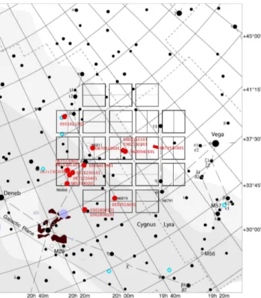
We aim to the highest homogeneity in the determination of the rotation period and in the characterization of the activity indicators, first of all the X-ray activity. To this end, we focus in this work on X-ray emitting stars detected by XMM-Newton with light curves from Kepler. We perform a positional match between the 3XMM-DR5 catalogue (Rosen et al. 2015) and the KeplerInput Catalogue (KIC, Brown et al. 2011), and then re-move non-stellar objects and objects with uncertain photometry. The 3XMM-DR5 catalogue includes data from 16 XMM-Newton pointings within the field of view (FoV) of the Kepler mission (see Table 1). Their sky position is shown in Fig. 1. The KeplerFoV covers∼ 105 square degrees; the 16 XMM-Newton observations which fall inside this FoV cover only∼ 2% of that area.

The KIC positional error (∼ 0.1′′_{) is negligible with respect}

to the error in the 3XMM-DR5 position (.4′′_{at3 σ). We select}

all the 3XMM-DR5 unique1sources that have a positional match (columns SC RA, SC DEC in 3XMM-DR5) with one or more

1 _{The 3XMM-DR5 Catalogue contains a row for each X-ray}

detec-tion. For a certain “unique” source (the astrophysical object), many

de-Fig. 1: The field of view (FoV) of the Kepler mission is respresented by the solid black squares. It is centered at RA=19 22 40.0 , DEC=+44 30 00.0 , between the Cygnus and the Lyra constellation. The FoVs of the sixteen 3XMM-DR5 ob-servations we analysed (Table 1) are reported as red circles; the red numbers represent the 3XMM-DR5 unique observation ID (OBS ID). The FoVs of some XMM-Newton observations are totally or partially overlapping.

KIC objects within a radius given by three times their 3XMM-DR5 individual (1 σ) positional error (column SC POSERR). We calculate the average probability of a chance association be-tween a 3DR5 source and a KIC source in each XMM-Newton field as P = 1 − eπµr2

, where µ is the numerical density of KIC sources in the field and has a typical value of 10−4_{sources/arcsec}2_{, andr is three times the average position}

error of the 3XMM-DR5 source. We obtain an average probabil-ity of chance association of∼ 0.8 %. This translates to ∼ 0.14 chance associations per XMM-Newton field, i.e. ∼ 2 spurious matches in the whole sample.

We select only the objects with a detection significance in 3XMM-DR5 (column DET ML) greater than6 (probability of a spurious detection< 0.025) in at least one EPIC instrument in the energy band8 (0.2 − 12.0 keV), removing the others from the sample (4 objects removed). We reject the 21 sources that are classified as “extended” in 3XMM-DR5 (flag EP EXTENT> 6). The resulting sample consists of145 matches. There are no mul-tiple associations, that is associations between a KIC object and two or more 3XMM-DR5 objects, or viceversa.

Within this sample, we aim to identify genuine stars, re-moving (1) galaxies and (2) stars that possibly suffer confu-sion (stars which are not resolved by Kepler) and contamina-tections (referred to different observations) of that object may be avail-able.

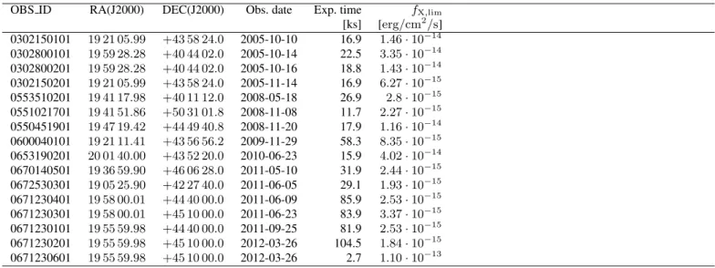
Table 1: XMM-Newton observations from the 3XMM-DR5 Catalogue in the Kepler FoV. Next to observation ID (col. 1), pointing center (cols. 2 and 3), observing date (cols. 4) and exposure time (col. 5), the flux sensitivity limit is given (col. 6) calculated as described in Sect. 2.2.

OBS ID RA(J2000) DEC(J2000) Obs. date Exp. time fX,lim

[ks] [erg/cm2_/s] 0302150101 19 21 05.99 +43 58 24.0 2005-10-10 16.9 1.46 · 10−14 0302800101 19 59 28.28 +40 44 02.0 2005-10-14 22.5 3.35 · 10−14 0302800201 19 59 28.28 +40 44 02.0 2005-10-16 18.8 1.43 · 10−14 0302150201 19 21 05.99 +43 58 24.0 2005-11-14 16.9 6.27 · 10−15 0553510201 19 41 17.98 +40 11 12.0 2008-05-18 26.9 2.8 · 10−15 0551021701 19 41 51.86 +50 31 01.8 2008-11-08 11.7 2.27 · 10−15 0550451901 19 47 19.42 +44 49 40.8 2008-11-20 17.9 1.16 · 10−14 0600040101 19 21 11.41 +43 56 56.2 2009-11-29 58.3 8.35 · 10−15 0653190201 20 01 40.00 +43 52 20.0 2010-06-23 15.9 4_{.02 · 10}−14 0670140501 19 36 59.90 +46 06 28.0 2011-05-10 31.9 2.44 · 10−15 0672530301 19 05 25.90 +42 27 40.0 2011-06-05 29.1 1.93 · 10−15 0671230401 19 58 00.01 +44 40 00.0 2011-06-09 85.9 2.53 · 10−15 0671230301 19 58 00.01 +45 10 00.0 2011-06-23 83.9 3_{.37 · 10}−15 0671230101 19 55 59.98 +44 40 00.0 2011-09-25 81.9 2_{.53 · 10}−15 0671230201 19 55 59.98 +45 10 00.0 2012-03-26 104.5 1_{.84 · 10}−15 0671230601 19 55 59.98 +45 10 00.0 2012-03-26 2.7 1_{.10 · 10}−13

tion from nearby bright sources. To this end, for each KIC ob-ject with a 3XMM-DR5 match, we search for a classification in the SIMBAD database2_{(Wenger et al. 2000) and we inspect the}

optical and infrared images, when available, using the Aladin service (Bonnarel et al. 2000; Boch & Fernique 2014). The fit of the Spectral Energy Distribution (SED) with a model for the stellar photospheric emission is also useful to identify galaxies in the sample (objects whose SED cannot be fit by a stellar model). Moreover, it allows us to determine the value of the stellar fun-damental parameters. The methods to remove non-stellar coun-terparts to the X-ray sources are explained in more detail in the following.

2.1. Spectral energy distribution (SED) 2.1.1. Multi-wavelength photometry

We extract the IR (2MASS J, H, K), optical (SLOAN g, r, i, z, Johnson U , B, V , Kepler Kp) and UV (GALEXF U V ,

N U V ) photometry for all stars of our sample from the KIC (Brown et al. 2011). Many sources lack photometry in one or more of these bands. We exclude from the sample the KIC jects for which no 2MASS IR photometry is available (2 ob-jects), since the wavelength range covered by 2MASS is crucial in order to perform a reliable spectral classification.

The visual inspection of the optical images via the Aladin server indicates that some stars suffer contamination from brighter objects located nearby. In such cases, even if they are recognised as distinct objects in the KIC, the photometry of the fainter one is expected to be significantly contaminated by the brighter one. Other stars suffer confusion between unresolved objects, i.e. they are not resolved in the KIC survey, but can be recognised as two objects through visual inspection of the opti-cal image. When the object is resolved in the UCAC-4 Catalogue (Zacharias et al. 2012), we replace the KIC photometry for these confused objects with the photometry provided by UCAC-4 for the brightest one. If no UCAC-4 photometry is available, we re-move the object from our sample (2 objects).

2 _{http://simbad.u-strasbg.fr/simbad/}

According to Pinsonneault et al. (2012), the SLOAN bands photometry reported in the KIC presents a significant systematic error, as observed comparing the KIC photometry in the bands g, r, i, z with the photometry reported in the Sloan Digital Sky Survey (SDSS-DR8) in the same bands, available for∼ 10% of the full KIC. Pinsonneault et al. (2012) give semi-empirical formulas to correct these systematics (their Eqs. 1, 2, 3, 4). We apply these corrections to the KIC SLOAN bands photometry of all the stars of our sample. The photometry for all the stars in our sample is reported in Table 6.

2.1.2. SED fitting

After the SEDs have been compiled, we fit them with photo-spheric BT-Settl models (Allard et al. 2012) within the Virtual Observatory SED Analyser(VOSA, Bayo et al. 2008). The pa-rameters of the BT-Settl models are:AV,log g, [F e/H] and Teff.

Due to parameter degeneracy it is not possible to determine all of them from the SED fit. Therefore we adopt for each star forAV,

log g and [F e/H] values taken from the literature (see Sect. 3), leavingTeffas the only free parameter. We thus obtain, for each

object, a best fitTeff under the hypothesis of a stellar model. As

the uncertainty on the effective temperature we assume the typ-ical dispersion of the five best fit values obtained in VOSA for each object (±200 K).

From the shape of their SED, combined with the visual in-spection of the Aladin images, sixteen objects are recognised as galaxies, and we remove them from our sample.

The whole sample selection procedure eventually results in a sample of125 3XMM-DR5 unique sources with a reliable stellar counterpart in Kepler, with a SED that is well-fitted by a stellar photosphere model.

2.2. X-ray flux limit

The sample of stars used in the present work has been selected based on the X-ray emission observed by XMM-Newton and as such is biased towards X-ray active stars. A fundamental step in order to understand the results presented in this work is,

there-fore, to provide an evaluation of the X-ray flux limit of the sam-ple. To this end, we first produce the EPIC PN3_{sensitivity map}

for each XMM-Newton observation of Table 1, for the energy range 0.2 − 2.0 keV using the task esensmap of the XMM-NewtonScience Analysis Software (SAS). The sensitivity map provides in each point of the FoV the limiting count rate needed to have a3 σ detection of a point source. We measure the limit-ing count rate in the centre of the FoV. We convert these num-bers into flux sensitivity limits (fX,lim) using WebPIMMS4

as-suming an APEC model with plasma temperature0.86 keV (see Sect. 5.1.2), abundance 0.2 in solar units and the galactic hy-drogen column density provided by Kalberla et al. (2005). The resulting numbers forfX,lim are reported in the last column of

Table 1. These values give an idea of the lower limit for the X-ray flux in these observations (median is∼ 6·10−15_erg/cm2_/s),

al-though we caution that the sensitivity varies strongly (up to about one order of magnitude) from the centre to the outer region of the FoV.

3. Fundamental stellar parameters

For 119 stars out of 125 we found literature values for effective temperature (Teff), visual absorption (AV) surface

gravity (log g), and metallicity ([Fe/H]) (in Huber et al. 2014 and Frasca et al. 2016). Huber et al. (2014) present a com-pilation of literature values for atmospheric properties (Teff,

log g and [Fe/H]) derived from different observational tech-niques (photometry, spectroscopy, asteroseismology, and ex-oplanet transits), which were then homogeneously fitted to a grid of isochrones from the Dartmouth Stellar Evolution Program (DSEP; Dotter et al. 2008), for a set of ∼ 200, 000 stars observed by the Kepler mission in Quarters 1 − 16. Frasca et al. (2016) present a systematic spectroscopic study of ∼ 50, 000 Kepler stars performed using the LAMOST tele-scope (Zhao et al. 2012). We compared the parameters obtained by Huber et al. (2014) and Frasca et al. (2016) for our sample, in particular the effective temperatures, and we found that they agree very well within the error bars. When available, however, we prefer the values obtained from Frasca et al. (2016) through the spectroscopic analysis, since in that work the stellar parame-ters have been evaluated using the same method for all the stars in their sample, while Huber et al. (2014) present a collection of values obtained in several works using different techniques.

Six stars in the sample do not have Teff reported in

Huber et al. (2014) or Frasca et al. (2016). For these6 stars we adopt asTeff the effective temperature of the best fit of the

indi-vidual SED with a model of the stellar photosphere, as described in Sect. 2.1. These stars are flagged with the ‘VOSA’ flag in col-umn12 of Table 7. Two out of these 6 stars have values for AV,

[Fe/H] and log g in Huber et al. (2014) or Frasca et al. (2016), and we use them in the SED fit. For the others, we adopt the median values of the distribution of AV in our sample (0.38),

[Fe/H]_⊙ (0.0) and log g (4.0). Similarly, for the additional 15 stars that have no literature value forAVwe adopt the median of

0.38 mag. The adopted values for the spectral parameters of all 125 stars are listed in Table 7.

In order to validate our SED fitting procedure we compare the obtainedTeff with the ones from the above-mentioned

lit-3

The EPIC (European Photon Imaging Camera) consists of three CCD detectors, two MOS and one PN, located at the focus of the three grazing incidence multi-mirror X-ray telescopes which constitute the main instrument onboard XMM-Newton .

4 _{http://heasarc.gsfc.nasa.gov/cgi-bin/Tools/w3pimms/w3pimms.pl} 3000 4000 5000 6000 7000 8000 05 10 15 20 25 30 Nu mb er 3000 4000 5000 6000 7000 8000 Teff, literature (K) 3000 4000 5000 6000 7000 8000 Tef f, VO SA (K )

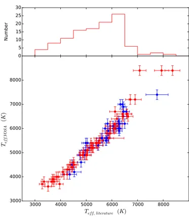
Fig. 2: In the upper panel, the distribution of the Teff of the

119 stars in our sample with Teff taken from the literature

(Huber et al. 2014; Frasca et al. 2016). In the lower panel, the comparison between theTeff drawn from the literature and the

ones obtained with the SED fitting is reported for the same sam-ple of stars. The colours represent the original work in which theTeffwas derived. Blue: Frasca et al. (2016); red: Huber et al.

(2014).

erature sources. The distribution ofTeff and the comparison

be-tween theTeffobtained from the SED fitting and the values in the

literature are reported in Fig. 2. Within the error bars, the agree-ment is for most stars very good, but the error bars of the values obtained by SED fitting are typically larger than the error bars in Huber et al. (2014) and especially in Frasca et al. (2016). This justifies our decision to adopt, when available, the literature val-ues forTeff. Given the effective temperature, we assign a

spec-tral type to each star according to Table 5 in Pecaut & Mamajek (2013). These values are given in Table 7.

3.1. Distance, mass and bolometric luminosity

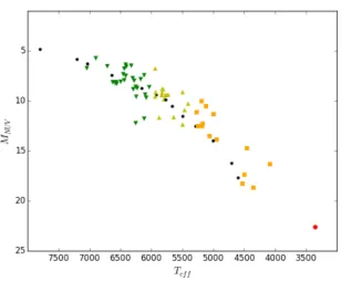
Fig. 3 shows our stellar sample together with the DSEP isochrones on thelog g vs log Teff plane. For each star, we

es-timate absolute J band magnitude, mass (M ) and bolometric luminosity (Lbol) by projecting its position and the related

un-certainties onto the isochrones (along the vertical axis) in Fig. 3. For this task we make use of DSEP isochrones in the range of 1.0 to 9.5 Gyr and for each star, we select the set of isochrones corresponding to the[Fe/H] value closest to the observed value. There are a few stars the position of which on thelog g vs log Teff

Fig. 3: log g − log Teff space with the set of isochrones from

DSEP and the stars of our sample (black circles) overplotted. Each stack of isochrones (lines in different grey-shades) corre-sponds to a given value of [F e/H] (−2.0, −1.5, −1.0, −0.5, 0.0, 0.2, 0.3, 0.5 from dark to pale).

DSEP isochrones. We mark them with a flag (‘DSEP outlier’) in Table 7.

Inverting the parallaxes provided in the Gaia-DR2 (Gaia Collaboration et al. 2018) we obtain the distances to our targets. While the overall quality of the Gaia-DR2 data is excellent, the mission is too complex to achieve optimal calibrations with less than two years of observations. As a result the Gaia-DR2 still contains many spurious astrometric solutions (Arenou et al. 2018). To remove putative problematic solutions we cleaned our dataset using the filters defined by Lindegren et al. (2018, appendix C, equations C-1 and C-2). Furthermore we used additional quality indicators of the solu-tions (astrometric excess noise> 0, astrometric gof al > 5) to discard other potential outliers. Two stars of our sample have no Gaia parallax while the solutions for further60 stars might not be reliable and were filtered out. For these 62 targets we derive the photometric distance from the comparison between the absolute magnitude and the observed J band magnitude. Comparison of the photometric and astrometric distances for the whole sample shows overall good agreement. For5 targets with reliable Gaia distances we found the J band distances to have lower uncertainties. In these cases we decided to adopt the J band distances. To summarize, throughout this work we use the Gaia distances for58 stars and the photometric J band distance for the remaining stars. Distance, mass and bolometric luminosity are reported for all125 stars in Table 7.

We classify the stars in our sample as main-sequence stars or giant stars according to theirlog g. In the log g vs log Teffspace,

the stars in our sample can be separated into two groups, cor-responding to the dwarf branch and to the giant branch, respec-tively (see Fig. 3). On this basis, we consider as main-sequence stars all the stars with log g ≥ 3.5, and as giants all the stars with log g < 3.5. With this criterion we find 19 giant stars. The four stars withoutlog g value in the literature can not be as-signed to these groups, and we eliminate them from the sample. These stars have a flag (*) in column12 of Table 7. This work is focused on main-sequence stars. Therefore, in the following, if not differently declared, we consider only the sample of the102

0 5 10 15 20 25 1 1.5 2 2.5 3 3.5 4

ALL

F

G

K

M

Fig. 4: Distribution of the adopted distances for the individual spectral types (from top to bottom: M, K, G, F) and for the whole sample of the main-sequence stars (bottom panel).

main-sequence stars. The distribution of their adopted distances is plotted in Fig. 4.

4. Analysis of Kepler light curves

The brightness modulation in the optical light curve due to the presence of inequally distributed spots on the rotating stellar surface enables the measurement of the stellar rotation period. Rotation periods, together with several photometric activity di-agnostics, are extracted from the Kepler light curves follow-ing the procedure described by Stelzer et al. (2016). The meth-ods developed therein for the analysis of M dwarf K2 mission lightcurves can readily be applied to the data from the main Keplermission, and we briefly resume the steps in Sect. 4.1.

To obtain a clean sample of stars for the rotation-activity study, periods originating from mechanisms different from the rotational brightness modulation due to starspots must be identi-fied and removed. In particular, our sample covers a broad range ofTeff in the Hertzsprung-Russell diagram, including the

inter-section of the main-sequence with the classical instability strip, where stellar pulsations are expected. Therefore, the light curves of some stars deserved a more detailed study in order to ascer-tain if pulsation (but also binarity) could be the real cause of the observed variability. We perform this study by means of the

Fourier decomposition (Poretti 1994) and the iterative analysis of the whole frequency spectrum (Van´ıˇcek 1971), described in Sect. 4.2.

4.1. Search for rotational periodicity

Briefly, the analysis consists of the following steps, imple-mented in an iterative procedure, which is described in detail by Stelzer et al. (2016): (1) period search with standard time-series analysis techniques (autocorrelation function [ACF] and Lomb-Scargle [LS] periodogram), (2) boxcar smoothing of the lightcurve and subsequent subtraction of the smoothed from the observed lightcurve, effectively removing the rotational modu-lation, (3) identification of ‘outlier’ data points in the ‘flattened’ lightcurve obtained from step (2) throughσ-clipping. The ‘out-liers’ comprise both instrumental artefacts and flares. The latter ones are identified by imposing three criteria: (i) a threshold (3σ) for the significance of the flare data points above the ‘flattened’ curve, (ii) criterion (i) applies to at least two consecutive such data points, and (iii) the maximum bin of the flare has at least a factor two higher flux than the last bin defining the flare. For a detailed description of the procedure used in each step of the analysis chain see Stelzer et al. (2016).

After the removal of the ‘outliers’ we repeat the period search, but in practice the applied methods are so robust that the cleaning of the lightcurves does not alter the result. What does change after the cleaning is the amplitude of the rotation cy-cle, when measured between maximum and minimum flux bin. However, as we describe below in Sect. 4.4, the preferred char-acterization of the spot cycle amplitude involves diagnostics that are little affected by the small fraction of ‘outlier’ data points. We perform this analysis for each Kepler observing Quarter in-dependently. This allows us to cross-check the results by com-paring the periods obtained from different Quarters, as explained in Sect. 4.3.

The determination of the rotation period for a given star proceeds in the following way. We use the routines A CORRELATE and SCARGLE in the IDL environment5_to

generate the ACF and LS periodogram. We work independently on the ACF and LS periodogram series. For each Kepler observ-ing Quarter, we inspect visually the ACF and LS periodogram generated by our procedure, and search for a signal of periodic variability (a sharp peak at a certain frequency, possibly followed by the related harmonics). If absent, we reject the Quarter from the analysis. In the ACF periodogram, we visually choose the highest peak of the series, which corresponds to the period of the modulation; this is generally the first one, or the second one if the light curve shows a double-humped pattern (as described below). In the LS periodogram, we likewise choose the highest peak.

For the majority of stars, the dominating periods derived with both techniques (ACF and LS) are consistent with each other. Deviations regard lightcurves with a double-humped shape. In this case, the light curve shows a double peak in at least some of the Kepler observing Quarters, while in others a single peak pattern may be observed. We interpret these features as the sig-nature of two groups of spots at a roughly antipodal position on the photosphere of the star, one of which may occasionally disappear. In this case, the ACF periodogram shows generally a first peak (corresponding to half the period) that has a lower am-plitude with respect to the second one, and this pattern repeats for the peaks corresponding to integer multiples of the first-peak

5 _{IDL is a product of the Exelis Visual Information Solutions, Inc}

period and of the second-peak period, respectively. In the Lomb-Scargle periodogram, the peak corresponding to the shorter pe-riod often has a larger amplitude than the longer-pepe-riod peak. The interpretation of these patterns as the effect of two groups of spots on the photosphere allows us to interpret the longer pe-riod of the two, corresponding to the double of the other, as the true rotation period of the star.

We obtain for each starNQperiods, whereNQis the number

of Quarters in which the star shows a periodic signal. This num-ber varies individually for the stars of our sample, independently for the ACF and the LS method. We adopt as the star’s period the median value of the periods obtained with the ACF method from the individual quarters.

4.2. Non-rotational periodicity

For some of the stars in our sample periodic variability is iden-tified that can not be explained with a simple spot pattern. In such cases the Fourier decomposition and the evaluation of the whole frequency spectra were very helpful. The frequency spec-tra of the genuine spotted stars are characterized by the harmon-ics of the rotational period and by low-frequency peaks due to the activity and rotational cycle-to-cycle period variations due to the shift in the spots’ latitude and to stellar differential rotation, and by some rotational cycle-to-cycle variation in the shape and amplitude of the lightcurve due to the variation of the area and shape of starspots. Other kinds of periodicity present different patterns.

We perform a dedicated anlysis of the light curves of the stars which do not show a clear variability pattern in order to classify their non-rotational variability. We find one multiperi-odic star showing the high-frequency pulsational regime ofδ Sct stars and three multiperiodic stars showing the low-frequency regime ofγ Dor stars. In the light curves of 2 stars the ampli-tudes of the even Fourier harmonics are much larger than those of the odd ones, as necessary to fit both the sharp minima and the large maxima shown by contact binaries. For3 stars it remains ambiguous if the variability is due to star spots or due to orbital motion in a contact binary; another2 stars display non-periodic variability that we could not classify. Finally,5 stars are likely rotational variables but displaying more than one period possibly indicating a binary composed of two spotted stars or a complex pattern with uncertain period. These16 stars are removed from the sample considered for the rotation-activity relation. A sum-mary of the number of main-sequence stars in each variability class for spectral type is given in Table 2.

4.3. Final sample of spotted stars

From the analysis described above, we can derive a rotation pe-riod for 74 stars in our sample, i.e. these stars are inhomoge-neously spotted. For the subsequent analysis, we also compute the Rossby number, defined asR0 = Prot/τconv, i.e. the ratio

between the rotation period and the convective turnover time. The convective turnover time is the characteristic time of cir-culation within a convective cell in the stellar sub-photosphere, and not directly observable. We calculate it from Teff using

Eq. 36 in Cranmer & Saar (2011), which is valid in the range 3300 K . Teff . 7000 K. All but two of the stars in our sample

are within this range ofTeff. The rotation periods and Rossby

numbers for all “spotted” stars are listed in Table 8. Our subse-quent photometric variability analysis is limited to this sample.

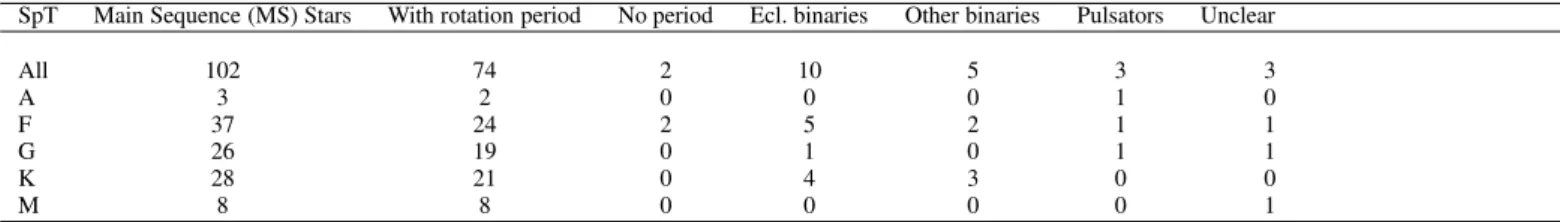
Table 2: Classification of the main-sequence stars in our sample according to the type of variability observed in the Kepler light curves.

SpT Main Sequence (MS) Stars With rotation period No period Ecl. binaries Other binaries Pulsators Unclear

All 102 74 2 10 5 3 3 A 3 2 0 0 0 1 0 F 37 24 2 5 2 1 1 G 26 19 0 1 0 1 1 K 28 21 0 4 3 0 0 M 8 8 0 0 0 0 1

4.4. Photometric activity diagnostics

From the analysis of the Kepler light curves we also obtain var-ious diagnostics for the stellar photospheric activity: the light curve amplitude and the standard deviation of the light curve.

The light curve amplitude is the photometric difference between the maximum and the minimum of the rotationally-modulated light curve, determined (in a light curve cleaned from flares) by the contrast between spotted and unspotted photo-sphere, combined with the inhomogeneous distribution of spots which causes the spot coverage of the observed stellar hemi-sphere to vary during the rotation. Analogous to Stelzer et al. (2016) and for consistency with the previous literature we de-cided to define the spot cycle amplitude as the range between the5th and 95th percentile of the observed flux values in a sin-gle rotation cycle (Rvar, see Basri et al. 2013), and we adopt

the modified definition ofRvar introduced by McQuillan et al.

(2013),Rper, which is the mean of the Rvar values measured

individually on all observed rotation cycles, expressed in per-cent. Cutting the upper- and lower-most5 % of the data points is another way of removing the ‘outliers’, such that no difference between theRvar values obtained from the original light curve

with the5th and 95th percentile and from the cleaned lightcurve is expected. We have verified this by comparing theRvarvalues

extracted from the light curves ‘cleaned’ from flares and outliers and theRvarvalues obtained from the original light curves.

The second activity diagnostic extracted from Kepler light curves that we use to characterize the variability during the spot cycle is the standard deviation of the whole light curve (Sph),

and the average of the standard deviations computed for time intervals k · Prot, withk integer, first defined by Mathur et al.

(2014b). Mathur et al. (2014b) have shown for a sample of22 stars that roughly after five rotation cycles the full range of flux variation is reached. Therefore, we computeSphandhSph,k=5i

for the stars in our sample. The standard deviation of the light curve was used as a proxy of magnetic activity also by He et al. (2015), in a study on the activity of two solar-like Kepler stars.

Finally, we have computed the standard deviation of the ‘flat-tened’ light curves (Sflat), measured on the light curves cleaned

from flares and outliers, and from which the rotational cycle has been removed (see description at the beginning of this Section). Stelzer et al. (2016) have established this parameter as an indi-cator for low-level unresolved astrophysical variability such as small unresolved flares and/or small and fast-changing spots for their sample of nearby M dwarfs observed in the K2 mission.

All these photometric activity diagnostics are listed in Table 8. It is worth noting here that the noise level in the ‘flat-tened’ lightcurve is expected to depend on the brightness of the star. In fact, Fig. 5 shows a correlation between the Kepler mag-nitude andSflat. As can be seen in Fig. 5, the apparent brightness

of our sample stars is on average larger for earlier spectral types. As a consequence, the noise tends to be smaller in those stars.

10 100 1000 10000 8 9 10 11 12 13 14 15 16 Sflat [ppm] Kp [mag] M K G F A

Fig. 5: Standard deviation of the ‘flattened’ lightcurve (Sflat) vs

Keplermagnitude. Shown is for each star the minimum ofSflat

from all quarters of observation.

This must be taken into account in the analysis of other kinds of variability; see e.g. Sect. 6.3.

5. X-ray and UV activity

As our sample is X-ray selected, every star in the sample has an associated X-ray detection. In the main-sequence sample,36 stars have also been detected in one or both of the UV energy bands (Near Ultra-Violet, NUV, and Far Ultra-Violet, FUV) of GALEX. In this section we analyse the X-ray and UV luminos-ity, and the corresponding ‘activity indexes’, defined as the ratio between the luminosity in the high-energy band and the bolo-metric luminosity of the star, as indicators of the stellar magnetic activity.

5.1. X-ray data analysis 5.1.1. Source X-ray luminosity

We calculate the X-ray luminosity of each star in the sample in the energy band0.2 − 2.0 keV (‘soft’ energy band, 3XMM-DR5 catalogue energy band 6). This range of energies corresponds approximately to the energy bands used in previous studies of the rotation-activity connection that were mainly based upon ROSAT data (e.g. Wright et al. 2011).

In the 3XMM-DR5 catalogue, there are many objects (‘sources’) that have been observed more than once: so, for a certain ‘source’, there can be many ‘detections’. Each row of the catalogue – which represents an individual detection of a cer-tain source – concer-tains a set of parameters referred to the tection itself, and a set of parameters averaged on all the de-tections available for that source. The catalogue provides the fluxes expected for a power law emission model for both the ‘detections’ and the ‘source’. However, the power law model, to which the fluxes given in 3XMM-DR5 refer, is not appropriate for describing the X-ray emission of late-type stars. Therefore, we re-calculate the X-ray flux in the bands0.2 − 2.0 keV from the EPIC PN count rate (or the MOS, if PN is not available), using the HEASARC online tool WebPIMMS, in which we as-sume for the X-ray emission of the stars a thermal APEC model (Smith et al. 2001). 3XMM-DR5 gives the ‘detection’ count rate for each of the three EPIC (European Photon Imaging Camera) instruments (PN, MOS1 and MOS2) on board the XMM-Newton mission, and the associated uncertainty, but it does not give the ‘source’ count rate. As described above, the ‘detection’ count rate is different from the ‘source’ count rate when the source has multiple detections in the catalogue. This happens for11 sources in our sample. So, we calculate the X-ray flux for these objects rescaling one of the individual ‘detection’ count rate for the fac-tor

f ₌ SC FLUX0.2−2.0 DET FLUX0_.2−2.0

(1) where SC FLUX0.2−2.0 and DET FLUX0.2−2.0 are

re-spectively the ‘source’ and ‘detection’ flux provided by 3XMM-DR5.

The APEC model in WebPIMMS requires as input parame-ters the hydrogen column density (NH), the metallicity and the

temperature of the emitting plasma. We estimate the hydrogen column density for each source from the visual absorptionAV

following Cardelli et al. (1989), as

NH= AV[mag] · 1.79 · 1021cm−2. (2)

We adopt an average abundance of0.2 in solar units, which is a typical value for the coronae of X-ray emitting late-type stars (see e.g. Pandey & Singh 2012). We calculate the count-to-flux conversion factor with WebPIMMS. To establish an operational kT , we fit the spectra of the brightest X-ray sources in XSPEC, and assume for all stars the kT value in the WebPIMMS grid (kT = 0.86 keV) which is closest to the average kT obtained from the spectral fits (kT = 0.83 keV). The spectral analysis of the brightest sources is described in the following.

5.1.2. Spectral analysis

We select the subsample of stars for which we have at least 200 events in the source extraction region in the three EPIC instruments together (PN+MOS1+MOS2). Excluding the stars classified as eclipsing or contact binaries, we have a sample of 19 stars. For each one, we extract the source and background spectrum in the energy band 0.3 − 10.0 keV, and perform a joint spectral analysis with XSPEC 12.8.1 (Arnaud 1996) of the spectra of all EPIC instruments available for that source. We fit the spectra with an absorbed one-temperature APEC model (phabs*apec) or an absorbed two-temperature APEC model (phabs*(apec+apec)). We set the coronal abundance to the typical value of0.2 in solar units (see above) to reduce the num-ber of free parameters and avoid degeneracy.

Two stars show a significant parameter degeneracy in their spectrum, so we remove them from the analysis. For the stars for which the model requires two temperatures, we calculate an average temperature weighted on the flux of the two APEC com-ponents. The results of the best fit for each of the17 stars, all characterized by a null-hypothesis probability> 0.3 %, are re-ported in Table 3. We calculate the averagekT over the 17 stars (< kT >= 0.83 keV).

With the parameters given in Sect. 5.1.1, we obtain from WebPIMMS the expected flux for each source. We then compare these fluxes with the fluxes obtained from the spectral analysis, for each of the17 sources for which the spectral fit in XSPEC was performed. For each of these stars we calculate the ratio be-tween the XSPEC flux and the flux from WebPIMMS. For PN, MOS1 and MOS2, we found an average ratio of respectively 0.91, 0.89, 1.00 in the soft energy band 0.2 − 2.0 keV. We cor-rect the fluxes obtained with WebPIMMS for the faint (< 200 counts) sources by multiplying them with this factor. This cor-rection is meant to obtain from WebPIMMS a flux that is, on average, as close as possible to the actual flux obtained from a spectral fit.

In the sample of17 bright stars, kT ranges from 0.49 keV to1.3 keV. This range is typical for active stars, and the actual plasma temperatures of the bulk of the faint stars is likely in the same range. This span of temperatures introduces an error in the flux calculated with the averagekT , allowing fluxes which are up to ∼ 2% lower or ∼ 15% higher than the one calculated from the average temperature of the bright stars. If the17 X-ray-brightest sources are not representative of our whole sample, these errors may be somewhat larger for the faint stars.

From the corrected fluxes we calculate the X-ray luminos-ity using the distances derived in Sect. 3.1. For each source we calculate the X-ray activity index as

AIX =

LX

Lbol

. (3)

The distributions of the X-ray luminosity and of the correspond-ing activity index in the soft energy band (0.2 − 2.0 keV) are reported in Fig. 6. The individual X-ray luminosities are listed in Table 9.

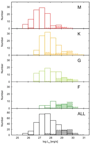
5.1.3. Considerations on the X-ray luminosity distribution We compare the distribution of the X-ray luminosity in the range 0.2 − 2.0 keV for the stars in our sample with those in the NEXXUS sample of Schmitt & Liefke (2004), which consists in a compilation of coronal X-ray emission for nearby late-type stars based on the ROSAT observatory. The distribution of the X-ray luminosity for our main-sequence sample and for the one from Schmitt & Liefke (2004) is plotted, for each spectral type and for the whole sample, in Fig. 7.

To first order we consider NEXXUS as a volume-limited sample of nearby stars, representing the full range of X-ray ac-tivity of the solar-like stellar population. Note, however, that Stelzer et al. (2013) showed that even in as small a volume as 10 pc around the Sun about 40 % of the M dwarfs have no X-ray detection in the RASS. From the comparison with our dis-tribution, it is evident that our sample presents a significant bias towards high X-ray luminosities most marked for the latest spec-tral types reflecting the mass (orTeff) dependence of X-ray

lu-minosity. The stars in our sample, which is flux-limited, are on average at a much greater distance (see Fig. 7, median distance for the whole sample: ∼ 500 pc). Therefore, we interpret the

Table 3: Best fit spectral parameters for the17 brightest X-ray sources (more than 200 counts) identified as rotational variables; parameters are for a phabs*apec or phabs*(apec+apec) model.

KIC ID SpT(a) _Counts(b) _{Model N}

H kT EM [cm−2_{] [keV] [cm}−3_] 5112508 M 520 phabs*apec _{∼ 0} 0.83 1_{.31 · 10}52 5113557 F 2088 phabs*apec 1_{.46 · 10}20 0.60 6_{.40 · 10}50 5653243 K 316 phabs*apec _{∼ 0} 0.80 5_{.86 · 10}52 6761532 G 226 phabs*apec 3.60 · 1020 _{0.63 2.43 · 10}52 7018708 G 2637 phabs*(apec+apec) 6.80 · 1020 _{0.29, 1.04 1.93 · 10}53_{, 2.24 · 10}53 8454353 M 1291 phabs*apec _{∼ 0} 0.99 9.69 · 1051 8517303 K 1763 phabs*apec 9.10 · 1020 _{1.06 1.10 · 10}54 8518250 K 434 phabs*(apec+apec) ∼ 0 0.94, 0.23 1.24 · 1051, 1.88 · 1051 8520065 F 764 phabs*(apec+apec) 2.33 · 1020 _{1.07, 0.54 4.30 · 10}53_{, 3.42 · 10}53 8584672 K 230 phabs*apec ∼ 0 0.83 1.21 · 1053 8647865 F 433 phabs*apec ∼ 0 0.49 1.60 · 1052 8713822 K 675 phabs*apec 1.43 · 1020 _{1.05 2.58 · 10}54 8842083 K 590 phabs*apec 1.1 · 1021 _{0.76 7.01 · 10}50 9048551 K 1634 phabs*apec ∼ 0 1.07 8.91 · 1051 9048949 K 844 phabs*apec ∼ 0 0.94 4.31 · 1051 9048976 K 285 phabs*apec ∼ 0 0.96 4.11 · 1051 11971335 G 696 phabs*apec ∼ 0 1.30 2.10 · 1053

(a)_{Spectral type has been evaluated from theT}

effaccording to Pecaut & Mamajek (2013). (b)_{This is the sum of the counts in the three EPIC instruments.}

Fig. 6: Distribution of the X-ray luminosity and of the X-ray ac-tivity index in the energy band0.2 − 2.0 keV for the 102 main-sequence stars.

bias of our sample towards active stars as due to both the X-ray selection and the large distances.

5.1.4. X-ray light curves

In order to study the variability of the X-ray emission and to search for X-ray flares, we analyse the light curves provided by the EXTraS (Exploring the X-ray Transient and variable Sky) project6 _{(De Luca et al. 2015). EXTraS was synchronized}

with 3XMM-DR4, while we are studying X-ray sources from 3XMM-DR5 in the Kepler field. Therefore, light curves for ob-servations 0671230201 and 0671230601 are not present in the public EXTraS database, but were produced for this work by the EXTraS team, using the EXTraS analysis pipeline.

EXTraS provides a set of uniform bin light curves with dif-ferent bin size, from 10 s up to 5000 s and an optimum bin size (chosen to have at least 25 counts in each bin), both for the source and the background extraction regions. In addition, EXTraS also provides light curves produced via an adaptive bin-ning, namely bayesian blocks (Scargle et al. 2013) algorithm for each source and for the related background region. This algo-rithm starts with an initial set of cells defined on the basis of the number of events in the source and background region, and pro-vides a final set of different-duration bins, each of which has a count rate that is not consistent, within3 σ, with the count rate of the adjacent bins.

In the EXTraS analysis pipeline, all the source light curves, both the ones obtained with the uniform bin algorithm and the bayesian blocks algorithm, are automatically fitted with a series of different models that account for simple variability patterns (constant, linear, quadratic, negative exponential, constant plus flare, constant plus eclipse). This is a standard algorithm that is part of the EXTraS pipeline, and it is applied to all the light curves in the same way. Its purpose is to provide a first-step in-dication of the kinds of variability possibly present in the light

6 _{The EXTraS project (www.extras-fp7.eu), aimed at the thorough}

characterization of the variability of X-ray sources in archival XMM-Newtondata, was funded within the EU seventh Framework Programme for a data span of 3 years starting in January 2014. The EXTraS consor-tium is lead by INAF (Italy) and includes other five institutes in Italy, Germany and the United Kingdom.

0 20 40 60 80 25 26 27 28 29 30 31

ALL

_F

_G

_K

_M

Fig. 7: Distribution of the X-ray luminosity in the energy band 0.2 − 2.0 keV, for the 102 main-sequence stars of the Kepler- XMM-Newton sample (hatched histograms) and for the NEXXUS stars from Schmitt & Liefke (2004) (solid line) for each spectral type class separately and for all spectral types com-bined.

curve, and not to perform a detailed modeling of the variability features observed, nor to determine their parameters. All results are in the database, and online searches can be performed with the query form.

5.1.5. X-ray flaring

For each X-ray source in our sample, we search for X-ray flares in the EXTraS light curves. First, we inspect the results of the fit performed on the light curves with different variability models by the EXTraS pipeline. As stated above, these results can be used for a first assessment for the kind of variability present in the light curve. If at least one among the uniform bin or adap-tive bin light curves is better fitted by a constant plus flare model (higher null-hypothesis probability) than the other models, this is a good indication of a possible flare. This flare model consists of a constant flux level over which a simple flare profile is su-perimposed, that is a steep linear flux increase, followed by an exponential decay.

The bayesian blocks light curves are particularly useful to detect flares, which appear as one or more blocks that show a higher flux than the preceeding and following blocks. If the flare occurred at the beginning or at the end of the observation, the bayesian blocks light curve may show only the rise phase or the decay phase. In this case, we rely on the uniform bin light curves to establish if the event is a true flare or not. We also require that the flare was observed in at least two of the EPIC instruments. The visual inspection of the light curves is however crucial in order to recognize genuine flares, so we inspect all the available EXTraS light curves for each star in our sample.

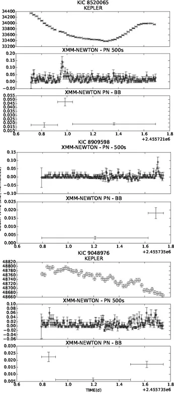
With this procedure, based on the EXTraS pipeline products we detect6 X-ray flares on 5 stars, and by visual inspection we identify an additional likely flare on a sixth star, KIC 7018131 (Figs. 8, and 9). In view of the low count statistics of the X-ray lightcurves some remarks on the individual events are in order. KIC 9048976 shows two possible flares: the bayesian blocks al-gorithm shows one block with a higher flux at the beginning and at the end of the light curve, impeding the observation of the full flare profile. KIC 8909598 also shows an X-ray flare at the end of the observation. The uniform bin light curves reveal a quite obvious flare profile both in PN and MOS2 cameras. However, this star does not have a reliable main-sequence classification (unknownlog g), so we do not consider it in the analysis. For KIC 9048551 the bayesian block algorithm identifies one flare event, but the uniform bin lightcurve shows evidence of sub-structure contemporaneous with two events seen in the Kepler band.

The X-ray flares shown in Fig. 8 have simultanous white-light flares in the Kepler white-light curves (see Sect. 6.3). Fig. 9 dis-plays the light curves for the X-ray flares without a simultaneous white-light counterpart revealed with the flare detection algo-rithm described in Sect. 4.1. Evidence for a weak increase of the optical brightness at times of the X-ray flare is, however, seen in all the contemporaneous Kepler lightcurves.

In Table 4 we report the start time of the X-ray flares (col. 2), according to the bayesian blocks light curve except for KIC 7018131, for which we infer the start time from the 500 s uniform bin light curve of EPIC/pn, since the bayesian blocks light curve has only one block. We also report the qui-escent (col. 3) and peak (col. 4) X-ray count rate, taken from the 500 s uniform bin light curve of EPIC/pn, together with the over-all number of white-light flares observed in the whole Kepler light curve for the star (col. 5), its white-light flare frequency (col. 6), the average, maximum and minimum peak amplitude of the Kepler flares (Apeak, photometric ratio between the peak bin

and the baseline of the flare, cols. 7 and 8). This parameter is discussed in more detail in Sect. 6.3.1.

5.2. UV activity

The KIC provides UV magnitudes obtained with the Galaxy Evolution Explorer (GALEX). The GALEX satellite performed imaging in two UV bands, far-UV (henceforth FUV; λeff =

1516 ˚A,∆λ = 268 ˚A , and near-UV (henceforth NUV;λeff =

2267 ˚A,∆λ = 732 ˚A). The KIC gives a NUV detection for71 stars from our main-sequence sample (i.e.70 %) and a FUV de-tection for 20 main-sequence stars (20 %). All but one of the stars with a FUV detection also have a NUV detection. The in-dividual values for the observed NUV and FUV luminosities are listed in cols. 3 and 4 of Table 9.

The SED fit provides UV fluxes for the stellar photosphere. In order to validate these measurements, we convert the NUV de-absorbed photospheric fluxes obtained from VOSA into

ab-Table 4: Parameters of the X-ray flares and Kepler flare characteristic of the X-ray flaring stars. The start time of each X-ray flare is reported, together with the peak and off-flare count rate. The number and the frequency of the white-light flares observed for the star is also given, together with the average, minimum and maximum peak amplitude of all its white-light flares in the Kepler light curve.

KIC ID Start time RateX,quiesc RateX,peak Nopt,flares Fopt,flares < log Apeak> Min-max log Apeak

(Julian day) (cts/s) (cts/s) (d−1₎ 7018131 2455718.31 0.006±0.011 0.035±0.019 5 0.005 -2.79 -2.89 / -2.67 8454353 2455829.96 0.036±0.020 0.263±0.048 297 0.211 -1.86 -0.36 /-2.69 8520065 2455721.96 0.020±0.016 0.140±0.040 0 0 0 0 8909598 2455736.55 0.004±0.011 0.090±0.003 7 0.022 -1.83 -1.43/-2.21 9048551 2455736.03 0.033±0.016 0.125±0.028 233 0.164 -2.41 -1.47/-2.92 9048976 2455735.94,2455736.80 0.009±0.013 0.06±0.02,0.060±0.024 137 0.097 -2.37 -1.57/-2.91

solute magnitudes and compare the relation between these mag-nitudes and theB − V colour (derived from Pecaut & Mamajek 2013) with the analogous relation observed for a set of photo-spheric NUV magnitudes provided by Findeisen et al. (2011) in their Table 1. Fig. 10 shows that our values are in good agree-ment with the ones of Findeisen et al. (2011).

For some stars in our sample the observed GALEX NUV and FUV fluxes are significantly higher than the prediction of the best-fitting photosphere model. This UV excess, i. e. the pos-itive difference between the observed UV flux (fUV,obs) and

the photospheric flux of the BT-Settl model in the same UV band (fUV,ph) represents the UV emission associated with

mag-netic activity processes in the stellar chromosphere. Following Stelzer et al. (2013), we calculate the corresponding UV activity index as AI′ UV= fUV,exc fbol = fUV,obs− fUV,ph fbol (4) wherefUV,exc is the UV excess flux attributed to activity, and

fbolis the bolometric flux. The bolometric flux is obtained from

interpolation on the DSEP isochrones, as described in Sect. 3. We calculate the UV excess in both the GALEX FUV and NUV band, where available. After trying different values and visually inspecting the SED, we find that a threshold of 13% on the ratio between the excess flux and the photospheric ex-pected flux is the best choice to select the stars with a true UV excess. We found45 main-sequence stars with a NUV excess, ten of them display also a FUV excess, and an additional4 have a FUV excess but no NUV excess. The NUV and FUV excess luminosities are provided in cols. 5 and 6 of Table 9.

6. Results and discussion

6.1. Rotation periods

For74 main-sequence stars out of 102 (73%) the Kepler light curve is dominated by the rotational brightness modulation due to starspots, with a period in the explored rangeProt < 90 d.

For the individual spectral types, the fraction of main-sequence stars with a rotational brightness modulation is: A66 % (2/3), F65 % (24/37), G 73 % (19/26), K 75 % (21/28) and M 100 % (8/8). Our period detection rate is higher with respect to other studies based on Kepler data (McQuillan et al. 2013, 2014,37% in the range3500 K < Teff < 6500 K, F ∼ 27%, G ∼ 25%, K

∼ 60%, M ∼ 80%; Stelzer et al. 2016, 73% for M dwarfs). This is probably an effect of the selection bias towards active (and thus strongly spotted) stars as well as the removal of giant stars from our sample.

In Table 2 a summary of the number of stars with rotation period from our analysis is reported for every spectral type,

to-gether with the number of stars with other types of brightness modulation patterns. We refer to Table 7 for the classification of the photometric variability for each star in the sample.

Only 54 stars out of 74 have previously reported periods from McQuillan et al. (2014), obtained from the same Kepler light curves. For the54 stars for which a rotation period is re-ported in McQuillan et al. (2014), those periods are consistent with our values within uncertainties. The remaining22 stars do not have any previously determined period in the literature. 6.2. Activity-rotation relation

In Fig. 11, we present the relation between the X-ray luminosity in the soft energy band0.2 − 2.0 keV and the rotation period, together with the relation between the X-ray activity index (de-fined in Eq. 3) and the Rossby number. A clear decrease in X-ray activity levels is observed for slower rotators. This effect is more evident in theAIx versus Rossby number plot, and produces a

‘kink’ in the distribution, which can be seen quite clearly in the overall sample of all stars, and also in the subsamples of K stars, while for M, G and F stars it is not obvious as these subsamples comprise only a limited range of rotation rates. The ‘kink’ sug-gests the presence of a correlated regime for slow rotators, and of a saturated regime for fast rotators, with a separation occurring at ∼ 8 d (from visual inspection). The wide range of LX and

AIXindependent ofProtfor the (generally fast rotating) F stars

is remarkable: it is possible that the F stars present a decoupling between rotation and activity because of their shallow convective zones. This group may also include active binary stars (RS CVn) with unknown contribution to the X-ray emission from the cool companions.

In Fig. 11 we show for comparison the literature compilation from Wright et al. (2011) and the previous empirical relations obtained by Pizzolato et al. (2003) based on a small sample with mostly spectroscopic rotation measurements (solid lines). The rotation periods in Wright et al. (2011) were collected from sev-eral works which use both spectroscopic and photometric tech-niques, and the X-ray fluxes were obtained from the analysis of data taken from different missions, such as XMM-Newton and ROSAT. We find excellent agreement of our more homo-geneous data with that study. Especially, the scatter clearly de-creases when X-ray luminosity and rotation period are replaced byAIxandR0, respectively. Contrary to previous work where

no uncertainties were estimated, we present here conservative error bars for our sample. These are dominated by the uncertain-ties in the distances of stars without Gaia parallax that are de-rived from mapping the stars in thelog g − log Teff diagram onto

the Dartmouth isochrones (see Sect. 3.1), i.e. they ultimately go back to the uncertainties in the spectroscopic parameters.

Fig. 8: Simultaneous Kepler and XMM-Newton EPIC PN light curves for the stars showing a simultaneous X-ray and white-light flare. The EPIC white-light curves produced by the EXTraS pipeline with 500 s uniform binning and with the bayesian blocks adaptive binning are plotted. The flare in the Kepler light curve of KIC 7018131 corresponds to a bump in the EPIC uni-form bin lightcurve which is, however, not significant at a 3σ level over the baseline, and not detected with the bayesian block algorithm.

Fig. 9: XMM-Newton EPIC PN light curves for the X-ray flares without a white-light counterpart detected by our flare-detection algorithm. Simultaneous Kepler light curves are not available for KIC 8909598.

The rotation-activity relation of M dwarfs in our sample can be compared to that of M dwarfs observed in the K2 mission studied by Stelzer et al. (2016) with an analogous approach. In Fig. 12 we show theLx− Protrelation for the two samples. Our

X-ray selection evidently excludes slowly rotating M stars in the non-saturated regime. This can also be seen from the comparison with the bimodal relation suggested by Pizzolato et al. (2003) (solid black line in Fig. 11) which is, however, itself extremely

Fig. 10: Absolute NUV magnitude versus Johnson colour B-V for the stars in our sample with a GALEX NUV detec-tion, for each spectral type, and for the values of Table 1 in Findeisen et al. (2011) (black dots). Different symbols represent the spectral type; red circles: M, orange squares: K, light-green triangle up: G, dark-green triangle down: F.

poorly defined. Recent M dwarf studies by Wright & Drake (2016) and Wright et al. (2018), also shown in the figure, used rotation periods measured with ground-based instruments. They cover the long-period ‘correlated’ region and are complementary to our Kepler study.

The scatter observed in the saturated regime of LX and

AIx for M stars of givenProt is large but consistent with that

observed by Wright et al. (2011), Pizzolato et al. (2003) and Stelzer et al. (2016), and probably due, at least in part, to the spectral type distribution within the M class, with cooler stars having lower X-ray luminosity. The scatter decreases when con-sidering the relation AIx versusR0. Because of the relatively

low statistics in our sample, in particular the low number of stars in the correlated regime, it would be difficult to establish with good confidence the turnover point between the correlated and saturated regime, nor the slope of the correlated part of the rela-tion.

6.3. Kepler activity diagnostics 6.3.1. Optical flares

We explore here the optical flaring activity measured in the Keplerlightcurves of the spotted stars. This analysis must con-sider that the sensitivity for detecting flares depends on the (qui-escent) brightness of the star and is different for each star. The criteria in our definition of flare include a≥ 3 σ upward devi-ation from the ‘flattened’ lightcurve (see Sect. 4.1). As a result of the relation betweenKpand spectral type in our sample

(evi-dent in Fig. 5), the minimum measurable flare amplitude (Apeak)

– defined here as the relative brightness difference between the flare peak and the ‘flattened’ lightcurve – shows a trend with spectral type (Fig. 13).

For a meaningful comparison of our sample which cov-ers a large range in brightness we must convert relative quan-tities, such asApeakandSflat, to absolute ones. The Kepler

pho-tometry is not flux calibrated. However, an approximate bright-ness can be associated to the ‘flattened’ lightcurve assuming that

this normalized ‘quiescent’ emission corresponds to the Kepler magnitude of the star. We convertKp to flux using the

zero-point and effective bandwidth provided at the filter profile ser-vice of the Spanish Virtual Observatory (SVO)7_{. Then we apply}

the distances derived in Sect. 3.1 to obtain the ‘quiescent’ lu-minosity in the Kepler band,LKp,0. Similarly, the flare ampli-tude is converted from its relative value (Apeak) to a

luminos-ity,∆LF,Kp = LKp,0· Apeak. The resulting relation between flare amplitude (in erg/s) and ‘quiescent’ luminosity is shown in Fig. 14. The lower envelope is defined by our flare detection threshold which is marked as a horizontal bar for each star and which is rising with increasing stellar luminosity. The A-type stars form an exception to this trend. They show lower flare am-plitudes than expected for theirLKp,0. This finding can easily be explained when the observed flares are attributed to unknown and unresolved later-type companion stars. In this scenario the actualLKp,0value of the flare-host would be lower making the true amplitude∆LF,Kphigher than measured. This would shift the data points to the left and upwards in Fig. 14.

For a given star, the range of flare luminosities,∆LF,Kp, ex-tends up to ∼ 2 orders of magnitude above the amplitude of the minimum observable flare. The range of flare amplitudes is smaller for G and F stars but this is probably related to the lack of sensitivity for the detection of low-luminosity flares. This is evident from consideration of theSflatvalues which set the

de-tection threshold (see Fig. 13 and 14).

One of the aims of our study is the investigation of a connec-tion between flaring activity and rotaconnec-tion rate. In their analogous study on M dwarfs observed in the K2 mission, Stelzer et al. (2016) have found a sharp transition in the optical flaring be-havior at a period of∼ 10 d. This transition is difficult to probe with this X-ray selected Kepler sample for two reasons: (1) the small number of slow rotators and (2) the broad range ofKp

translating into a dishomogeneous flare detection threshold. If we restrict our sample to M dwarfs which span a relatively nar-row range in optical brightness (c.f. Fig. 5), the relative flare am-plitudes and the flare frequencies are consistent with the results obtained by Stelzer et al. (2016) but we are covering only the fast periods up to the presumed transition (see Fig. 15). The av-erage flare frequency of the M stars in our sample (0.12 flares/d) is in excellent agreement with the average flare frequency in Stelzer et al. (2016) calculated over theProtrange (Prot.10 d)

covered by the Kepler M stars (0.11 flares/d). This shows that our Kepler sample, albeit highly incomplete at the slow rotation / low activity side, is representative for fast rotating and active M dwarfs.

Analogous to the study of Stelzer et al. (2016) on K2 lightcurves, the sampling time of 29.4 min of the Kepler lightcurves used in this work, together with the characteristics of the flare search algorithm (see Sect. 4.3), prevent the detec-tion of flares with duradetec-tion below ∼ 1 h. As a consequence, we detect mostly flares with large-amplitude and relatively long duration. It can be suspected that there is a significant popula-tion of smaller and shorter flares that cannot be observed, due to the long cadence of the light curves and to the flare-extraction pipeline. Therefore, the flare frequencies of Fig. 15 and Table 5 likely represent a lower limit to the actual values.

6.3.2. X-ray versus white-light flares

As described in Sect. 5.1.5 we find7 X-ray flares on 6 stars. For these events the count rate at the flare peak (as measured from

26 27 28 29 30 31 0.1 1 10 100 log L x [erg/s] Prot [d] -7 -6 -5 -4 -3 -2 0.001 0.01 0.1 1 10 log L x /Lbol R0 26 27 28 29 30 31 0.1 1 10 100 log L x [erg/s] Prot [d] -7 -6 -5 -4 -3 -2 0.001 0.01 0.1 1 10 log L x /Lbol R0 26 27 28 29 30 31 0.1 1 10 100 log L x [erg/s] Prot [d] -7 -6 -5 -4 -3 -2 0.001 0.01 0.1 1 10 log L x /Lbol R0 26 27 28 29 30 31 0.1 1 10 100 log L x [erg/s] Prot [d] -7 -6 -5 -4 -3 -2 0.001 0.01 0.1 1 10 log L x /Lbol R0 26 27 28 29 30 31 0.1 1 10 100 log L x [erg/s] Prot [d] -7 -6 -5 -4 -3 -2 0.001 0.01 0.1 1 10 log L x /Lbol R0

Fig. 11: X-ray activity versus rotation for the full sample, M-, K-, G-, and F-type stars (from top to bottom). Left panel: X-ray luminosity in the energy band0.2 − 2.0 keV versus Kepler Right panel: X-ray activity index versus Rossby number. Colours and symbols follow the convention defined in Fig. 10. The stars in the sample of Wright et al. (2011) are shown as small black dots. The solid lines represent the best-fit relations between X-ray emission and rotation period found by Pizzolato et al. (2003) for stellar mass ranges corresponding approximately to spectral types.

25 26 27 28 29 30 1 10 100 − − − Pizzolato+03 relation for 0.22...0.60 M_sun log L x [erg/s] Prot [d] K7...M2 M3...M4 M5...M6

Fig. 12:LX vsProt for M dwarfs: red – this work, black – K2

sample from Stelzer et al. (2016) (their Fig. 15), green – stars published by Wright & Drake (2016) and Wright et al. (2018). The solid line represents the best-fit rotation/activity relation from Pizzolato et al. (2003) in the range0.22 − 0.60 M⊙.

−4 −3 −2 −1 0 10 100 1000 10000 log(A peak ) S_flat [ppm] M K G F A

Fig. 13: Relative peak amplitudes of all detected optical flares in the Kepler lightcurves measured with respect to the ‘flattened’ lightcurve. The grey line denotes our threshold for flare detection set to3 · Sflat.

Table 5: Mean values and standard deviations measured for pho-tometric activity diagnostics in the Kepler / XMM-Newton sam-ple.

SpT Nf/day logRper[%] Sph[ppm]

A 0.001 _−1.02 3_{.47 · 10}2 F 0.01 _−0.74 1_{.10 · 10}3 G 0.02 0.01 5.39 · 103 K 0.04 0.25 8.69 · 103 M 0.12 0.46 1.10 · 104 27 28 29 30 31 32 33 31 32 33 34 log( ∆ LF,K p ) [erg/s] log(LKp,0) [erg/s] M K G F A

Fig. 14: Absolute flare amplitudes versus quiescent luminosity represented by the Kepler magnitude associated with the ‘flat-tened’ lightcurve; see text for details.

−4 −3 −2 −1 0 0 0.5 1 1.5 2 log(A peak ) log P_rot [d] 0 0.1 0.2 0.3 0 0.5 1 1.5 2 Nflares /day log Prot [d]

Fig. 15: Relative flare amplitudes (Apeak; top panel) and flare

frequency (bottom panel) versus rotation period for the M stars in our Kepler sample (red) and for the M stars of the K2 sample presented by Stelzer et al. (2016) (black).