Advance Access publication 2017 January 11
BAT AGN Spectroscopic Survey IV. Near-infrared coronal lines, hidden
broad lines and correlation with hard X-ray emission
Isabella Lamperti,
1‹Michael Koss,
1,2Benny Trakhtenbrot,
1Kevin Schawinski,
1Claudio Ricci,
3Kyuseok Oh,
1Hermine Landt,
4Rog·erio Riffel,
5Alberto Rodr·guez-Ardila,
6Neil Gehrels,
7Fiona Harrison,
8Nicola Masetti,
9,10Richard Mushotzky,
11Ezequiel Treister,
3Yoshihiro Ueda
12and Sylvain Veilleux
111Institute for Astronomy, Department of Physics, ETH Zurich, Wolfgang-Pauli-Strasse 27, CH-8093 Z¤urich, Switzerland 2Institute for Astronomy, University of Hawaii, 2680 Woodlawn Drive, Honolulu, HI 96822, USA
3Instituto de Astrof·sica, Facultad de F·sica, Ponti cia Universidad Cat·olica de Chile, Casilla 306, Santiago 22, Chile 4Centre for Extragalactic Astronomy, Department of Physics, Durham University, South Road, Durham DH1 3LE, UK
5Departamento de Astronomia, Universidade Federal do Rio Grande do Sul., Av. Bento Gonc‚alves 9500, Porto Alegre, RS, Brazil 6Laborat rio Nacional de Astrof·sica, Rua dos Estados Unidos 154, Bairro das Nac‚oes, CEP 37504-364 Itajub·a, MG, Brazil 7NASA Goddard Space Flight Center, Greenbelt, MD 20771, USA
8Cahill Center for Astronomy and Astrophysics, California Institute of Technology, Pasadena, CA 91125, USA 9INAF Istituto di Astro sica Spaziale e Fisica Cosmica di Bologna, via Gobetti 101, I-40129 Bologna, Italy 10Departamento de Ciencias F·sicas, Universidad Andr·es Bello, Fern·andez Concha 700, Las Condes, Santiago, Chile 11Department of Astronomy and Joint Space-Science Institute, University of Maryland, College Park, MD 20742, USA 12Department of Astronomy, Kyoto University, Kyoto 606-8502, Japan
Accepted 2017 January 9. Received 2017 January 9; in original form 2016 September 30
ABSTRACT
We provide a comprehensive census of the near-infrared (NIR, 0.8 2.4 µm) spectroscopic properties of 102 nearby (z < 0.075) active galactic nuclei (AGN), selected in the hard X-ray band (14 195 keV) from the Swift-Burst Alert Telescope survey. With the launch of the
James Webb Space Telescope, this regime is of increasing importance for dusty and obscured
AGN surveys. We measure black hole masses in 68 per cent (69/102) of the sample using broad emission lines (34/102) and/or the velocity dispersion of the CaIItriplet or the CO
band-heads (46/102). We nd that emission-line diagnostics in the NIR are ineffective at identifying bright, nearby AGN galaxies because [FeII] 1.257 µm/Pa and H22.12 µm/Br
identify only 25 per cent (25/102) as AGN with signi cant overlap with star-forming galaxies and only 20 per cent of Seyfert 2 have detected coronal lines (6/30). We measure the coronal line emission in Seyfert 2 to be weaker than in Seyfert 1 of the same bolometric luminosity suggesting obscuration by the nuclear torus. We nd that the correlation between the hard X-ray and the [SiVI] coronal line luminosity is signi cantly better than with the [OIII] 5007
luminosity. Finally, we nd 3/29 galaxies (10 per cent) that are optically classi ed as Seyfert 2 show broad emission lines in the NIR. These AGN have the lowest levels of obscuration among the Seyfert 2s in our sample (log NH< 22.43 cm 2), and all show signs of galaxy-scale
interactions or mergers suggesting that the optical broad emission lines are obscured by host galaxy dust.
Key words: galaxies: active quasars: emission lines quasars: general galaxies: Seyfert
infrared: galaxies X-rays: galaxies.
E-mail:[email protected] Ambizione Fellow.
Zwicky Fellow.
1 INTRODUCTION
The near-infrared (NIR) spectral regime (0.8 2.4 µm) provides nu-merous emission lines for studies of active galactic nuclei (AGN) and has the advantage to be 10 times less obscured than the op-tical (Veilleux2002). For example, the vibrational and rotational
BASS IV: NIR spectroscopy
541
modes of H2 can be excited by UV uorescence (Black & van Dishoeck1987; Rodr·guez-Ardila et al.2004; Rodr·guez-Ardila, Riffel & Pastoriza2005; Riffel et al.2013), shock heating (Hol-lenbach & McKee1989) and heating by X-rays, where hard X-ray photons penetrate into molecular clouds and heat the molecular gas (Maloney, Hollenbach & Tielens1996). The [FeII] emission in AGN can be produced by shocks from the radio jets or X-ray heating, while in star-forming galaxies (SFGs) the [FeII] emission is produced by photoionization or supernovae shocks (Rodr·guez-Ardila et al.2004).
NIR emission-line diagnostics (e.g. Larkin et al. 1998; Rodr·guez-Ardila et al.2004; Riffel et al.2013; Colina et al.2015) are based on the close relation between the line ratios [FeII] 1.257 µm/Pa and H2 2.12 µm/Br , and the nuclear black hole activity. In principle, the low levels of dust attenuation in the NIR imply that such line diagnostics can be used even among highly reddened objects. However, several studies (e.g. Dale et al.2004; Martins et al.2013) found that this diagnostic is not effective in separating SFGs from AGN.
The NIR regime also includes the hydrogen Pa and Pa emis-sion lines, which by virtue of being less obscured may at times ( 30 per cent of sources) present a hidden broad-line region (BLR), in galaxies with narrow optical H and/or H lines (e.g. Veilleux, Goodrich & Hill1997; Onori et al.2014; Smith, Koss & Mushotzky2014; La Franca et al.2015). Onori et al. (2016) recently studied a sample of 41 obscured (Sy2) and intermediate-class AGN (Sy1.8 1.9) and found broad Pa , Pa or HeIlines in 32 per cent (13/41) of the sources. The study of Landt et al. (2008) compared the width of the Paschen and Balmer lines (in terms of full width at half-maximum FWHM) and found that H is generally broader than Pa . One possible reason for this trend is the presence of the H red shelf (e.g. De Robertis1985; Marziani et al.1996), which origi-nates from FeIImultiplets (Veron, Goncalves & Veron-Cetty2002). Another possibility is that the broad Balmer lines originate from a region closer to the black hole than the Paschen lines (Kim, Im & Kim2010).
The NIR broad Paschen emission lines can be used to derive black hole mass (MBH) estimates, based on their luminosities and widths, following a similar approach to that based on the optical Balmer lines (e.g. Kim et al.2010; Landt et al.2011b,2013). Alternatively, the size of the BLR (RBLR), and therefore MBH, can also be estimated using the 1-µm continuum luminosity (Landt et al.2011a) or the hard-band X-ray luminosity (e.g. La Franca et al.2015), again mimicking similar methods to those put forward for the Balmer lines (Greene et al.2010). For obscured AGN, the spectral region surrounding the CaIItriplet of absorption features (0.845 0.895 µm; e.g. Rothberg & Fischer2010; Rothberg et al.2013) and CO band-heads in the H and K band (e.g. Dasyra et al.2006a,b,2007; Kang et al.2013; Riffel et al. 2015) are useful regions to measure the stellar velocity dispersion ( ) to infer MBHfollowing the MBH relation (Ferrarese & Merritt2000; Tremaine et al.2002; McConnell & Ma2012; Kormendy & Ho2013).
Moreover, the NIR regime is important because it includes several high-ionization (>100 eV) coronal lines (CLs) generated through photoionization by the hard UV and soft X-ray continuum produced by AGN or by shocks (e.g. Rodr·guez-Ardila et al.2002, 2011). CLs tend to be broader than low-ionization emission lines emitted in the narrow line region (NLR), but narrower than lines in the BLR (400 km s 1< FWHM < 1000 km s 1). This suggests that they are produced in a region between the BLR and the NLR (Rodr·guez-Ardila et al.2006). M¤uller-S·anchez et al. (2011) investigated the spatial distribution of CLs and found that the size of the coronal
line region (CLR) only extends to a distances of <200 pc from the centre of the galaxy (Mazzalay, Rodr·guez-Ardila & Komossa2010; M¤uller-S·anchez et al.2011).
Recently, it has been found that high-ionization optical emission lines, such as [OIII] 5007, are only weakly correlated with AGN X-ray luminosity or with bolometric luminosity (Berney et al.2015; Ueda et al.2015). The considerable intrinsic scatter in this relation (0.6 dex) may be related to physical properties of the NLR such as covering factor of the NLR (e.g. Netzer & Laor 1993), den-sity dependence of [OIII] (Crenshaw & Kraemer2005), differing ionization parameter (Baskin & Laor2005) and spectral energy dis-tribution (SED) shape changes with luminosity (Netzer et al.2006). Other possible reasons are AGN variability (Schawinski et al.2015), dust obscuration, or contamination from star formation. CLs in the NIR, by virtue of the higher ionization potentials (IPs) and the mi-nor sensitivity to dust obscuration, provide an additional method to study this correlation.
In this work, we aim to study the NIR properties of one of the largest samples of nearby AGN (102) from the Swift/Burst Alert Telescope (BAT) survey selected at 14 195 keV (Baumgartner et al.2013) as part of the BAT AGN Spectroscopic Survey (BASS). This sample, by virtue of its selection, is nearly unbiased to ob-scuration up to Compton-thick levels (Koss et al.2016). The rst BASS paper (Koss et al., submitted) detailed the optical spectro-scopic data and measurements. The second BASS paper (Berney et al.2015) studied the large scatter in X-rays and high-ionization emission lines like [OIII]. Additionally, all of the AGN have been analysed using X-ray observations including the best available soft X-ray data in the 0.3 10-keV band from XMM-Newton, Chandra, Suzakuor Swift/XRT and the 14 195 keV band from Swift/BAT, which provide measurements of the obscuring column density (NH; Ricci et al.2015, submitted). Therefore, we are able to compare the NIR properties of these AGN with their optical and X-ray char-acteristics, to better understand AGN variability and obscuration. Throughout this work, we use a cosmological model with = 0.7, M= 0.3 and H0= 70 km s 1Mpc 1to determine distances. How-ever, for the most nearby sources in our sample (z < 0.01), we use the mean of the redshift-independent distance in Mpc from the NASA/IPAC Extragalactic Database (NED), whenever available.
2 DATA AND REDUCTION 2.1 Sample
The Swift/BAT observatory carried out an all-sky survey in the ultrahard X-ray range (>10 keV) that, as of the rst 70 months of operation, has identi ed 1210 objects (Baumgartner et al.2013) of which 836 are AGN. The majority ( 90 per cent) of BAT-detected AGN are relatively nearby (z < 0.2).
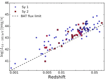
We limited our NIR spectra sample to 102 nearby AGN with redshift z < 0.075 to ensure high-quality observations for both Seyfert 1 and Seyfert 2. In our sample, there are 69 Seyfert 1 and 33 Seyfert 2. A full list of the AGN can be found in Tables1 3. Fig.1shows the distribution of the hard X-ray luminosity of the AGN in our sample as a function of redshift. Most of the AGN (96) are listed in the Swift/BAT 70-month catalogue (Baumgartner et al.2013) with an additional six AGN from the Palermo 100-month BAT catalogue (Cusumano et al.2010) and the upcoming Swift/BAT 104-month catalogue (Oh et al., in preparation).
The goal of our survey was to use the largest available NIR spec-troscopic sample of Swift/BAT sources using dedicated observations and published data. More than half (55 per cent, 56/102) of the AGN MNRAS 467, 540 572 (2017)
Table 1. Spectra from the IRTF observations.
IDa Counterpart name Redshift Slit size Slit size Date Air mass Exp. time Typeb Hc
(arcsec) (kpc) (yy-mm-dd) (s) (mag)
316 IRAS 05589+2828 0.033 0.8 0.54 11-04-12 1.23 2160 1.2 399 2MASX J07595347+2323241 0.0292 0.8 0.48 12-03-14 1.01 2160 1.9 10.3 434 MCG +11-11-032 0.036 0.8 0.59 12-03-14 1.42 2160 2 11.4 439 Mrk 18 0.0111 0.8 0.18 11-04-12 1.33 2520 1.9 10.5 451 IC 2461 0.0075 0.8 0.13 12-03-14 1.11 1080 2 10.1 515 MCG +06-24-008 0.0259 0.8 0.43 12-03-19 1.12 2520 2 10.8 517 UGC 05881 0.0205 0.8 0.34 11-04-12 1.01 1800 2 10.9 533 NGC 3588 NED01 0.0268 0.8 0.44 11-04-12 1.02 1620 2 10.6 548 NGC 3718 0.0033 0.8 0.05 10-06-11 1.24 4140 1.9 7.9 586 ARK 347 0.0224 0.8 0.37 12-03-19 1.17 2520 2 10.7 588 UGC 7064 0.025 0.8 0.41 12-03-19 1.58 2340 1.9 10.3 590 NGC 4102 0.0028 0.8 0.05 10-06-11 1.26 1200 2 7.8 592 Mrk 198 0.0242 0.8 0.40 12-03-19 1.16 2520 2 11.2 593 NGC 4138 0.003 0.8 0.05 10-06-11 1.24 3240 2 8.3 635 KUG 1238+278A 0.0565 0.8 0.93 12-03-02 1.07 3600 1.9 11.8 638 NGC 4686 0.0167 0.8 0.28 11-04-12 1.22 3240 2 9.1 659 NGC 4992 0.0251 0.8 0.42 11-04-12 1.04 3960 2 10.3 679 NGC 5231 0.0218 0.8 0.36 10-06-12 1.07 1800 2 10.4 682 NGC 5252 0.023 0.8 0.38 10-06-12 1.12 1800 2 9.9 686 NGC 5273 0.0036 0.8 0.06 10-06-12 1.19 1800 1.5 8.8 687 CGCG 102 048 0.0269 0.8 0.44 12-03-19 1.35 2160 2 11.3 695 UM614 0.0327 0.8 0.54 11-04-12 1.53 1200 1.5 11.6 712 NGC 5506 0.0062 0.8 0.10 10-06-11 1.21 1200 1.9 8.2 723 NGC 5610 0.0169 0.8 0.28 11-04-12 1.02 2520 2 10.1 734 NGC 5683 0.0362 0.8 0.60 12-03-13 1.19 2160 1.2 11.8 737 2MASX J14391186+1415215 0.0714 0.8 1.17 11-04-12 1.08 3420 2 13.1 738 Mrk 477 0.0377 0.8 0.62 11-04-12 1.49 1440 1.9 12.1 748 2MASX J14530794+2554327 0.049 0.8 0.80 10-06-11 1.10 1800 1 12.5 754 Mrk 1392 0.0361 0.8 0.60 11-04-12 1.56 1200 1.5 11.1 783 NGC 5995 0.0252 0.8 0.42 11-06-16 1.24 1800 1.9 9.5 883 2MASX J17232321+3630097 0.04 0.8 0.66 11-06-16 1.04 960 1.5 11.4 1041 2MASS J19334715+3254259 0.0583 0.8 0.96 10-06-11 1.08 1680 1.2 1042 2MASX J19373299 0613046 0.0107 0.8 0.18 11-09-14 1.16 720 1.5 9.7 1046 NGC 6814 0.0052 0.8 0.09 11-09-14 1.19 1200 1.5 7.8 1077 MCG +04-48-002 0.0139 0.8 0.23 10-06-12 1.02 1800 2 9.9 1099 2MASX J21090996 0940147 0.0277 0.8 0.46 11-09-14 1.23 1800 1.2 10.6 1106 2MASX J21192912+3332566 0.0507 0.8 0.83 11-09-15 1.04 1800 1.5 11.5 1117 2MASX J21355399+4728217 0.0259 0.8 0.43 10-06-11 1.32 1800 1.5 11.5 1133 Mrk 520 0.0273 0.8 0.45 10-06-12 1.08 1800 2 10.8 1157 NGC 7314 0.0048 0.8 0.08 11-09-15 1.43 1440 1.9 8.3 1158 NGC 7319 0.0225 0.8 0.37 10-06-11 1.28 1800 2 10.4 1161 Mrk 915 0.0241 0.8 0.40 11-09-15 1.2 1440 1.9 10.4 1178 KAZ 320 0.0345 0.8 0.57 10-06-12 1.08 1800 1.5 12.1 1183 Mrk 926 0.0469 0.8 0.77 10-06-11 1.42 1800 1.5 10.8 1196 2MASX J23272195+1524375 0.0465 0.8 0.76 11-09-15 1 1440 1.9 11.1 1202 UGC 12741 0.0174 0.8 0.29 10-06-11 1.15 1200 2 10.8 1472 CGCG 198 020 0.0269 0.8 0.44 10-06-12 1.13 1800 1.5 1570 NGC 5940 0.0339 0.8 0.56 10-06-12 1.31 1800 1
Notes.aSwift/BAT 70-month hard X-ray survey ID (http://swift.gsfc.nasa.gov/results/bs70mon/). bAGN classi cation following Osterbrock (1981).
cH 20 mag arcsec 2isophotal ducial elliptical aperture magnitudes from the 2MASS extended source catalogue.
were observed as part of a targeted campaigns using the SpeX spec-trograph (Rayner et al.2003) at the NASA 3-m Infrared Telescope Facility (IRTF; 49 sources) or with the Florida Multi-object Imag-ing Near-IR Grism Observational Spectrometer (FLAMINGOS; El-ston 1998) on the Kitt Peak 4-m telescope (seven sources). The targets were selected at random based on visibility from the north-ern sky. Additionally, we included spectra from available archival observations. We used 15 spectra from Riffel, Rodr·guez-Ardila & Pastoriza (2006), 14 spectra from Landt et al. (2008), two spectra
from Rodr·guez-Ardila et al. (2002) and one spectrum from Riffel et al. (2013) observed with IRTF. We used three spectra observed by Landt et al. (2013) and 13 publicly available spectra from Mason et al. (2015) observed with the Gemini Near-Infrared Spectrograph (GNIRS; Elias et al.2006) on the 8.1-m Gemini North telescope. We note there is some bias towards observing more Seyfert 1 in our sample compared to a blind survey of BAT AGN ( 50 per cent Seyfert 1) because some archival studies focused on Seyfert 1 (e.g. Landt et al.2008).
BASS IV: NIR spectroscopy
543
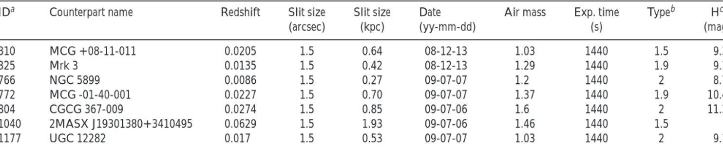
Table 2. Spectra from the FLAMINGOS observations.
IDa Counterpart name Redshift Slit size Slit size Date Air mass Exp. time Typeb Hc
(arcsec) (kpc) (yy-mm-dd) (s) (mag)
310 MCG +08-11-011 0.0205 1.5 0.64 08-12-13 1.03 1440 1.5 9.3 325 Mrk 3 0.0135 1.5 0.42 08-12-13 1.29 1440 1.9 9.1 766 NGC 5899 0.0086 1.5 0.27 09-07-07 1.2 1440 2 8.7 772 MCG -01-40-001 0.0227 1.5 0.70 09-07-07 1.37 1440 1.9 10.4 804 CGCG 367-009 0.0274 1.5 0.85 09-07-06 1.6 1440 2 11.3 1040 2MASX J19301380+3410495 0.0629 1.5 1.93 09-07-06 1.46 1440 1.5 1177 UGC 12282 0.017 1.5 0.53 09-07-07 1.03 1440 2 9.1
Notes.aSwift/BAT 70-month hard X-ray survey ID (http://swift.gsfc.nasa.gov/results/bs70mon/). bAGN classi cation following Osterbrock (1981).
cH 20 mag arcsec 2isophotal ducial elliptical aperture magnitudes from the 2MASS extended source catalogue. We used the [OIII] redshift, optical emission-line measurements
and classi cation in Seyfert 1 and Seyfert 2 from Koss et al. (sub-mitted). Optical counterparts of BAT AGN and the 14 195-keV measurements were based on Baumgartner et al. (2013). We also used the NH and 2 10-keV ux measurements from Ricci et al. (2015, submitted). The optical observations were not taken simul-taneously to the NIR observations but come from separate targeted campaigns or public archives.
2.2 NIR spectral data
While the data were taken from a number of observational cam-paigns, we maintain a uniform approach to data reduction and analysis. The observations were taken in the period 2010 2012. A summary of all the observational set-ups can be found in Table4. All programs used standard A0V stars with similar air masses to provide a benchmark for telluric correction. The majority of ob-servations were done with the cross-dispersed mode of SpeX on the IRTF using a 0.8 arcsec 15 arcsec slit (Rayner et al.2003) covering a wavelength range from 0.8 to 2.4 µm. The galaxies were observed in two positions along the slit, denoted position A and position B, in an ABBA sequence by moving the telescope. This provided pairs of spectra that could be subtracted to remove the sky emission and detector artefacts. For 16 objects, we have duplicate observations. In these cases, we chose the spectrum with the higher signal-to-noise ratio (S/N) in the continuum.
2.2.1 Targeted spectroscopic observations
For new observations, the data reduction was performed using stan-dard techniques withSPEXTOOL, a software package developed espe-cially for IRTF SpeX observations (Cushing, Vacca & Rayner2004). The spectra were tellurically corrected using the method described by Vacca, Cushing & Rayner (2002) and theIDLroutine Xtell-cor, using a Vega model modi ed by deconvolution with the spec-tral resolution. The routine Xcleanspec was used to remove regions of the spectrum that were completely absorbed by the at-mosphere. The spectra were then smoothed using a Savitzky Golay routine, which preserves the average resolving power. We used the smoothed spectra for the measurements of the emission lines, whereas for the absorption lines analysis we used the unsmoothed spectra. Further details are provided in Smith et al. (2014) and in the appendix.
We also have seven spectra observed with the FLAMINGOS spectrograph at Kitt Peak over the wavelength range 0.9 2.3 µm using two set-ups, one with the JH grism and the other with the K
grism both using a 1.5-arcsec slit. The spectra were rst at- elded, wavelength calibrated, extracted and combined usingIRAFroutines. Then telluric corrections and ux calibration were done in the same way as the IRTF observations using Xtellcorgeneral from SPEXTOOL. The FLAMINGOS spectrograph has limitations in its cooling system and this induced thermal gradients and lower S/N particularly in the K band, making this region unusable for analysis. Information about these observations is given in Tables1and2. 2.2.2 Archival observations
The archival observations from the IRTF were reduced usingSPEX -TOOL in the same way as the targeted observations. Additional archival NIR spectra were from GNIRS at the Gemini North obser-vatory observed with the cross-dispersed (XD) mode covering the 0.85 2.5-µm wavelength range processed using GeminiIRAFand the XDG-NIRS task (Mason et al.2015). Information about the archival observations is given in Table3.
3 SPECTROSCOPIC MEASUREMENTS
In this section, we present the spectroscopic measurements. First, we explain the emission lines tting method we used to measure the emission-line ux and FWHM (Section 3.1). Then, we describe absorption lines tting method that we apply to measure the stellar velocity dispersion (Section 3.2).
3.1 Emission lines measurements
We t our sample of NIR spectra in order to measure the emission-line ux and FWHM. We use PySpecKit, an extensive spec-troscopic analysis toolkit for astronomy, which uses a Levenberg Marquardt algorithm for tting (Ginsburg & Mirocha 2011). We
t separately the Pa14 (0.84 0.90 µm), Pa (0.90 0.96 µm), Pa (0.96 1.04 µm), Pa (1.04 1.15 µm), Pa (1.15 1.30 µm), Br10 (1.30 1.80 µm), Pa (1.80 2.00 µm) and Br (2.00 2.40 µm) spectral regions. An example t is found in Fig.2. Before applying the tting procedure, we deredden the spectra using the galactic extinction value EB Vgiven by the IRSA Dust Extinction Service1
and a function from the PySpecKit tool.
We employ a rst-order power-law t to model the continuum. For each spectral region, we estimated the continuum level from the entire wavelength range, except where the emission lines are located (–20 ¯ for the narrow lines and –150 ¯ for the broad 1http://irsa.ipac.caltech.edu/applications/DUST/docs/background.html
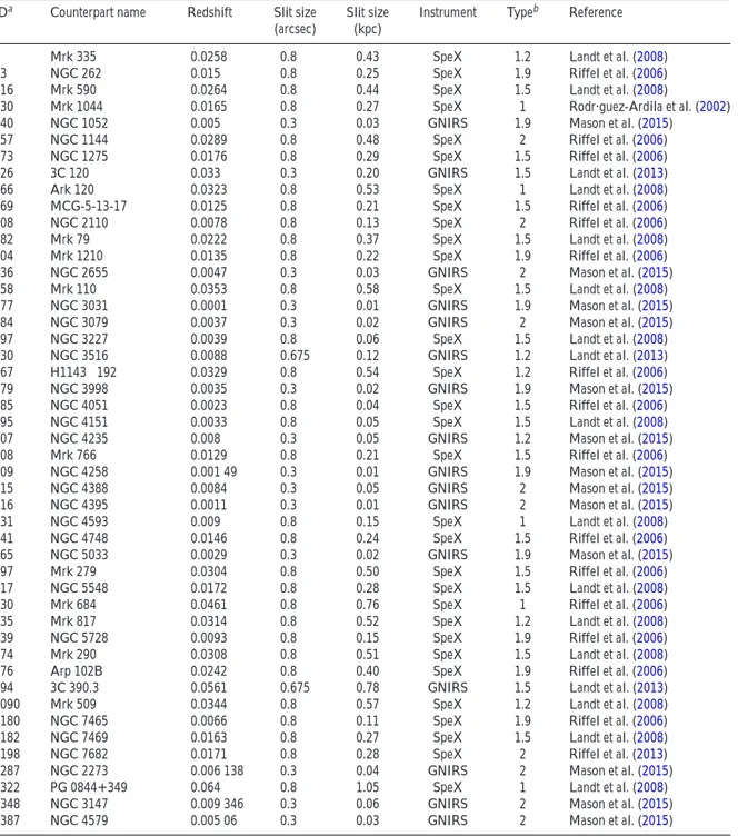
Table 3. Archival observations.
IDa Counterpart name Redshift Slit size Slit size Instrument Typeb Reference
(arcsec) (kpc)
6 Mrk 335 0.0258 0.8 0.43 SpeX 1.2 Landt et al. (2008)
33 NGC 262 0.015 0.8 0.25 SpeX 1.9 Riffel et al. (2006)
116 Mrk 590 0.0264 0.8 0.44 SpeX 1.5 Landt et al. (2008)
130 Mrk 1044 0.0165 0.8 0.27 SpeX 1 Rodr·guez-Ardila et al. (2002)
140 NGC 1052 0.005 0.3 0.03 GNIRS 1.9 Mason et al. (2015)
157 NGC 1144 0.0289 0.8 0.48 SpeX 2 Riffel et al. (2006)
173 NGC 1275 0.0176 0.8 0.29 SpeX 1.5 Riffel et al. (2006)
226 3C 120 0.033 0.3 0.20 GNIRS 1.5 Landt et al. (2013)
266 Ark 120 0.0323 0.8 0.53 SpeX 1 Landt et al. (2008)
269 MCG-5-13-17 0.0125 0.8 0.21 SpeX 1.5 Riffel et al. (2006)
308 NGC 2110 0.0078 0.8 0.13 SpeX 2 Riffel et al. (2006)
382 Mrk 79 0.0222 0.8 0.37 SpeX 1.5 Landt et al. (2008)
404 Mrk 1210 0.0135 0.8 0.22 SpeX 1.9 Riffel et al. (2006)
436 NGC 2655 0.0047 0.3 0.03 GNIRS 2 Mason et al. (2015)
458 Mrk 110 0.0353 0.8 0.58 SpeX 1.5 Landt et al. (2008)
477 NGC 3031 0.0001 0.3 0.01 GNIRS 1.9 Mason et al. (2015)
484 NGC 3079 0.0037 0.3 0.02 GNIRS 2 Mason et al. (2015)
497 NGC 3227 0.0039 0.8 0.06 SpeX 1.5 Landt et al. (2008)
530 NGC 3516 0.0088 0.675 0.12 GNIRS 1.2 Landt et al. (2013)
567 H1143 192 0.0329 0.8 0.54 SpeX 1.2 Riffel et al. (2006)
579 NGC 3998 0.0035 0.3 0.02 GNIRS 1.9 Mason et al. (2015)
585 NGC 4051 0.0023 0.8 0.04 SpeX 1.5 Riffel et al. (2006)
595 NGC 4151 0.0033 0.8 0.05 SpeX 1.5 Landt et al. (2008)
607 NGC 4235 0.008 0.3 0.05 GNIRS 1.2 Mason et al. (2015)
608 Mrk 766 0.0129 0.8 0.21 SpeX 1.5 Riffel et al. (2006)
609 NGC 4258 0.001 49 0.3 0.01 GNIRS 1.9 Mason et al. (2015)
615 NGC 4388 0.0084 0.3 0.05 GNIRS 2 Mason et al. (2015)
616 NGC 4395 0.0011 0.3 0.01 GNIRS 2 Mason et al. (2015)
631 NGC 4593 0.009 0.8 0.15 SpeX 1 Landt et al. (2008)
641 NGC 4748 0.0146 0.8 0.24 SpeX 1.5 Riffel et al. (2006)
665 NGC 5033 0.0029 0.3 0.02 GNIRS 1.9 Mason et al. (2015)
697 Mrk 279 0.0304 0.8 0.50 SpeX 1.5 Riffel et al. (2006)
717 NGC 5548 0.0172 0.8 0.28 SpeX 1.5 Landt et al. (2008)
730 Mrk 684 0.0461 0.8 0.76 SpeX 1 Riffel et al. (2006)
735 Mrk 817 0.0314 0.8 0.52 SpeX 1.2 Landt et al. (2008)
739 NGC 5728 0.0093 0.8 0.15 SpeX 1.9 Riffel et al. (2006)
774 Mrk 290 0.0308 0.8 0.51 SpeX 1.5 Landt et al. (2008)
876 Arp 102B 0.0242 0.8 0.40 SpeX 1.9 Riffel et al. (2006)
994 3C 390.3 0.0561 0.675 0.78 GNIRS 1.5 Landt et al. (2013)
1090 Mrk 509 0.0344 0.8 0.57 SpeX 1.2 Landt et al. (2008)
1180 NGC 7465 0.0066 0.8 0.11 SpeX 1.9 Riffel et al. (2006)
1182 NGC 7469 0.0163 0.8 0.27 SpeX 1.5 Landt et al. (2008)
1198 NGC 7682 0.0171 0.8 0.28 SpeX 2 Riffel et al. (2013)
1287 NGC 2273 0.006 138 0.3 0.04 GNIRS 2 Mason et al. (2015)
1322 PG 0844+349 0.064 0.8 1.05 SpeX 1 Landt et al. (2008)
1348 NGC 3147 0.009 346 0.3 0.06 GNIRS 2 Mason et al. (2015)
1387 NGC 4579 0.005 06 0.3 0.03 GNIRS 2 Mason et al. (2015)
Notes.aSwift/BAT 70-month hard X-ray survey ID (http://swift.gsfc.nasa.gov/results/bs70mon/). bAGN classi cation following Osterbrock (1981).
lines). For the modelling of the emission lines, we assume Gaussian pro les. The emission lines that we t in each spectral region are listed in TableA1in the appendix. The positions of the narrow lines are tied together. They are allowed to be shifted by a maximum of 8 ¯ ( 160 km s 1) from the systemic redshift. The redshift and widths of the narrow lines are also tied together. As an initial input value for the width of the narrow lines, we used the width of the [SIII] 0.9531-µm line, which is the strongest narrow emission line in the 0.8 2.4-µm wavelength range. We set the maximum FWHM of the narrow lines to be 1200 km s 1.
For the Paschen, Brackett and HeI 1.083-µm lines, we allow the code to t the line with a narrow component (FWHM < 1200 km s 1) and a broad component (FWHM > 1200 km s 1). We tied the width of the narrow component to the width of the other narrow lines present in the same spectral region. We also tied together the broad-line width of the Paschen lines that lie in the same tting region. The broad components are allowed to be shifted by a maximum of 30 ¯ ( 600 km s 1) from the theoretical position. This large velocity shift is motivated by the observations of a mean velocity shift of the broad H to the systemic redshift of
BASS IV: NIR spectroscopy
545
Figure 1. Distribution of the hard X-ray luminosity of the BAT AGN with respect to the redshift. The redshift is taken from NED. The dashed line shows the ux limit of the BAT 70-month survey over 90 per cent of the sky (1.34 10 11erg cm2s 1).
109 km s 1with a scatter of 400 km s 1in a sample of 849 quasars (Shen et al.2016). The largest velocity shifts are 1000 km s 1. We corrected the FWHM for the instrumental resolution, subtracting the instrumental FWHM from the observed FWHM in quadrature.
For line detection, we adopted an S/N of 3 compared to the surrounding continuum as the detection threshold. For each spectral region, we measured the noise level taking the dispersion of the continuum in a region without emission lines. In a few cases near blended regions with strong stellar absorption features (e.g. [SiVI]), a line detection seemed spurious by visual inspection even though it was above the detection limit. We have noted those with a ag and quote upper limits for these sources. If the S/N of the broad component of a particular line was below the threshold, we re-ran the tting procedure for the spectral region of this line, without including a broad component. We inspected by eye all the spectra to verify that the broad component was not affected by residuals or other artefacts. After visual inspection, we decided to t seven spectra with only a narrow component for Pa .
To estimate the uncertainties on the line uxes and widths, we performed a Monte Carlo simulation. We repeated the tting pro-cedure 10 times, adding each time an amount of noise randomly drawn from a normal distribution with the deviation equal to the noise level. Then, we computed the median absolute deviation of the 10 measurements and we used this value as an estimate of the error at the one-sigma con dence level. We inspected visually all
emission-line ts to verify proper tting and we assigned a quality ag to each spectral t. We follow the classi cation nomenclature by visual inspection of the rst BASS paper (Koss et al., submit-ted). Quality ag 1 refers to spectra that have small residuals and very good t. Flag 2 means that the t is not perfect, but it is still acceptable. Flag 3 is assigned to bad t for high S/N source due to either the presence of broad-line component or offset in emission lines. Flag 9 refers to spectra where no emission line is detected. Flag 1 means lack of spectral coverage. The emission lines uxes and FWHM are listed in Tables10 19.
3.2 Galaxy templates tting
We used the Penalized Pixel-Fitting (PPXF) code (Cappellari & Em-sellem2004) to extract the stellar kinematics from the absorption-line spectra. This method operates in the pixel space and uses a maximum penalized likelihood approach to derive the line-of-sight velocity distributions (LOSVD) from kinematical data (Mer-ritt 1997). First the PPXFcode creates a model galaxy spectrum by convolving a template spectrum with a parametrized LOSVD. Then, it determines the best- tting parameters of the LOSVD by minimizing the 2value, which measures the agreement between the model and the observed galaxy spectrum over the set of good pixels used in the tting process. Finally,PPXFuses the best- tting spectra to calculate from the absorption lines.
We used the same spectra as those used in Section 3.1, dered-shifted to the rest frame. Here, we concentrate on three narrow wavelength regions where strong stellar absorption features are present: CaT region (0.846 0.870 µm), CO band-heads in the H band (1.570 1.720 µm) and CO band-heads in the K band (2.250 2.400 µm). The absorption lines present in these three wavelength ranges are listed in TableA2in the appendix. For the spectra from the FLAMINGOS spectrograph, we measured only from the CO band-heads in the H band, due to limited wavelength coverage.
ThePPXF code uses a large set of stellar templates to t the galaxy spectrum. We used the templates from the Miles Indo U.S. CaT Infrared (MIUSCATIR) library of stellar spectra (R¤ock et al.2015,2016). They are based on the MIUSCAT stellar popu-lations models, which are an extension of the models of Vazdekis et al. (2010), based on the Indo U.S., MILES (S·anchez-Bl·azquez et al.2006) and CaT (Cenarro et al.2001) empirical stellar libraries (Vazdekis et al.2012). The IR models are based on 180 empirical stellar spectra from the stellar IRTF library. This library contains the spectra of 210 cool stars in the IR wavelength range (Cushing, Rayner & Vacca2005; Rayner, Cushing & Vacca2009). The sample is composed of stars of spectral types F, G, K, M, AGB-, carbon- and S-stars, of luminosity classes I V. Some of the stars were discarded Table 4. Summary of instrumental set-ups.
Reference Telescope Instrument Nspectra Slit size Grating Resolving Wavelength
(arcsec) (l per mm) power range (µm)
This work IRTF SpeX 48 0.8 800 0.8 2.4
This work KPNO FLAMINGOS 7 1.5 1000 1.0 1.8
Riffel et al. (2006) IRTF SpeX 15 0.8 800 0.8 2.4
Landt et al. (2008) IRTF SpeX 14 0.8 800 0.8 2.4
Rodr·guez-Ardila et al. (2002) IRTF SpeX 1 0.8 800 0.8 2.4
Riffel et al. (2013) IRTF SpeX 1 0.8 800 0.8 2.4
Mason et al. (2015) Gemini North GNIRS 6 0.3 31.7 1300 0.9 2.5
7 0.3 31.7 1800 0.9 2.5
Landt et al. (2013) Gemini North GNIRS 2 0.675 31.7 750 0.9 2.5
1 0.3 31.7 1800 0.9 2.5
Table 5. Relations of CLs ([SiVI] and [SVIII]) and [OIII] and [SIII] emission with the 14 195-keV emission and 2 10-keV emission.
Flux 1 Flux 2 Sample N (dex) RPear pPear p-value
(1) (2) (3) (4) (5) (6)
Sy1 62 0.53 0.57 1.1 10 6
[OIII] 0.5007 µm X-ray 14 195 keV Sy2 26 0.75 0.41 0.04
All 88 0.67 0.49 1.3 10 6
Sy1 26 0.41 0.58 0.001 0.16
[SiVI] 1.962 µm X-ray 14 195 keV Sy2 7 0.26 0.54 0.21 0.84
All 33 0.39 0.57 0.0004 0.18
Sy1 25 0.48 0.57 0.003 0.88
[SVIII] 0.9915 µm X-ray 14 195 keV Sy2 4 0.02 0.98 0.02 (sample too small)
All 29 0.48 0.53 0.003 0.85
Sy1 48 0.42 0.64 1.0 10 6 0.65
[SIII] 0.9531 µm X-ray 14 195 keV Sy2 17 0.41 0.44 0.07 0.47
All 65 0.44 0.59 1.8 10 7 0.42
Sy1 58 0.53 0.59 1.2 10 6
[OIII] 0.5007 µm X-ray 2 10 keV Sy2 25 0.57 0.65 0.0004
All 83 0.64 0.58 1.1 10 8
Sy1 26 0.38 0.66 0.0002 0.04
[SiVI] 1.962 µm X-ray 2 10 keV Sy2 6 0.36 0.11 0.83 0.01
All 32 0.40 0.58 0.0004 0.47
Sy1 24 0.44 0.69 0.0002 0.20
[SVIII] 0.9915 µm X-ray 2 10 keV Sy2 3 0.121 0.33 0.79 (sample too small)
All 27 0.47 0.61 0.0007 0.87
Sy1 42 0.43 0.55 0.0001 0.85
[SIII] 0.9531 µm X-ray 2 10 keV Sy2 15 0.39 0.70 0.003 0.96
All 57 0.42 0.6 1.2 10 6 0.38
[OIII] 0.5007 µm [SiVI] 1.962 µm All 33 0.60 0.5 0.003
[SVIII] 0.9915 µm [SiVI] 1.962 µm All 22 0.20 0.88 9.0 10 8
[SIII] 0.9531 µm [SiVI] 1.962 µm All 26 0.33 0.80 1.1 10 6
Notes. (1) AGN type; (2) size of the common sample in which Flux 1, Flux 2 and [OIII] ux are available; (3) standard deviation and (4) Pearson R coef cient of the log Flux1 log Flux 2 relation; (5) Pearson p-value coef cient of the log Flux1 log Flux 2 relation; (6) p-value of the null hypothesis that this correlation coef cient and the [OIII] correlation coef cient obtained from independent parent samples are equal. All coef cients are measured for the sample that has both CL emission and [OIII] observations.
Table 6. Relations of CLs ([SiVI] and [SVIII]), [SIII] and [OIII] luminosities with the 14 195-keV emission and 2 10-keV emission.
Luminosity 1 Luminosity 2 N (dex) RPear pPear p-value
(1) (2) (3) (4) (5)
[OIII] 0.5007 µm X-ray 14 195 keV All 88 0.67 0.73 8.7 10 16
[SiVI] 1.962 µm X-ray 14 195 keV All 34 0.41 0.86 5.1 10 11 0.006 [SVIII] 0.9915 µm X-ray 14 195 keV All 29 0.49 0.83 2.9 10 8 0.916
[SIII] 0.9531 µm X-ray 14 195 keV All 65 0.48 0.83 2.5 10 17 0.002
[OIII] 0.5007 µm X-ray 2 10 keV All 83 0.64 0.75 1.9 10 16
[SiVI] 1.962 µm X-ray 2 10 keV All 32 0.41 0.87 1.6 10 10 0.019
[SVIII] 0.9915 µm X-ray 2 10 keV All 27 0.46 0.86 1.1 10 8 0.744
[SIII] 0.9531 µm X-ray 2 10 keV All 57 0.49 0.84 2.1 10 16 0.002
Notes. (1) Size of the common sample in which both Luminosity 1 and Luminosity 2 are available; (2) standard deviation and (3) Pearson R coef cient of the log Flux1 log Flux 2 relation; (4) Pearson p-value coef cient of the log Flux1 log Flux 2 relation; (5) p-value of the
null hypothesis that this correlation coef cient and the [OIII] correlation coef cient obtained from independent parent samples are equal. because of their unexpected strong variability, strong emission lines
or not constant baseline. The IR models cover the spectral range 0.815 5.000 µm at a resolving power R = 2000, which corresponds to a spectral resolution of FWHM 150 km s 1( 60 km s 1) equivalent to 10 ¯ at 2.5 µm (R¤ock et al.2015). A comparison with Gemini Near-Infrared Late-type stellar (GNIRS) library (Winge,
Riffel & Storchi-Bergmann2009) in the range 2.15 2.42 µm at R = 5300 5900 (resolution of 3.2 ¯ FWHM) is provided in the appendix. The spectral templates are convolved to the instrumental resolution of the observed spectra under the assumption that the shapes of the instrumental spectral pro les are well approximated by Gaussians.
BASS IV: NIR spectroscopy
547
Table 7. Relations of CLs and [SIII] luminosity with the 14 195-keV emission and 2 10-keV emission.
Line 2 10 keV 14 195 keV
Nundet Ndet X-ray-to-line Slope Intercept Ndet X-ray-to-line Slope Intercept
ratio ratio (1) (2) (3) (4) (5) (6) (7) (8) (9) [SIII] 0.9531 µm 6 57 227 1.20 – 0.11 11.30 – 4.78 65 587 1.11 – 0.10 7.81 – 4.43 [CaVIII] 2.3210 µm 76 8 7913 1.00 – 0.53 4.04 – 22.7 8 16448 0.67 – 0.37 67.74 – 16.01 [SiVI] 1.962 µm 42 32 1247 1.02 – 0.13 4.02 – 5.92 34 3217 0.83 – 0.13 0.75 – 5.75 [SVIII] 0.9915 µm 62 27 2756 1.18 – 0.15 11.31 – 6.52 29 5472 1.00 – 0.15 4.03 – 6.35 [SIX] 1.2520 µm 76 18 4177 1.00 – 0.22 3.92 – 9.45 18 9239 0.91 – 0.17 0.16 – 7.53 [FeXIII] 1.0747 µm 84 4 3754 0.44 – 0.70 20.43 – 30.08 4 8886 0.54 – 1.01 15.6 – 43.37 [SiX] 1.4300 µm 79 17 3481 0.96 – 0.17 1.77 – 7.42 18 8877 1.02 – 0.23 5.14 – 9.9
Notes. (1) Number of sources with no line detection in clean atmospheric regions for which the upper limits are measured; (2) size of the sample in which both
line luminosity and 2 10-keV intrinsic X-ray luminosity are measured; (3) mean 2 10-keV X-ray-luminosity-to-line-luminosity ratio for the sources with line detection (upper limits are not considered); (4) slope a and (5) intercept b of the ordinary least squares (OLS) bisector t log LLine= a log L2 10 keV+ b for the sources with line detection; (6) size of the sample in which both line luminosity and 14 195-keV X-ray luminosity are available; (7) mean 14 195-keV X-ray-luminosity-to-line-luminosity ratio for the sources with line detection (upper limits are not considered); (8) slope a and (9) intercept b of the OLS bisector t log LLine= a log L14 195 keV+ b for the sources with line detection.
We applied a mask when tting stellar templates around the following emission lines: Pa14 (in the CaT region), [FeII] 16436, [FeII] 16773 and Br11 16811 (in the H band), and [CaVIII] 23210 (in the K band). Since the [CaVIII] 23210 emission line overlaps with the CO(3 1) 23226 absorption line, we decided to mask the region around this line only if the emission line was detected. Also for the Pa14 line, we decided to mask the line only if the emission line was detected, because it is in the same position of the CaII 8498 absorption line and therefore it is in a critical region for the measurement of the velocity dispersion. We set the width of the emission lines mask to 1600 km s 1for the narrow lines and to 2000 km s 1for the Brackett and Paschen lines (Br11 and Pa14). The error on the velocity dispersion ( ) is the formal error (1 ) given by thePPXFcode. The error is in the range 1 20 per cent of the values.
All absorption lines ts were inspected by eye to verify proper tting. We follow the nomenclature of tting classi cation of the rst BASS paper (Koss et al., submitted). We assigned the quality ag 1 to the spectra that have small residuals and very good t of the absorption lines (average error = 6 km s 1). Quality ag 2 refers to the spectra that have larger residuals and errors in the velocity dispersion value (average error = 12 km s 1), but the absorption lines are well described by the t. For spectra where the error of the velocity dispersion value is >50 km s 1and the t is not good, we assigned the ag 9.
4 RESULTS
We rst compare the FWHM of broad Balmer and Paschen lines (Section 4.1). Then, we discuss AGN that show hidden broad lines in the NIR spectrum but not in the optical (Section 4.2). Next, we measure the velocity dispersion (Section 4.3) and black hole masses (Section 4.4). In Section 4.5, we apply NIR emission-line diagnostics to our sample. Then, we discuss the presence of CLs in the AGN spectra (Section 4.6). Finally, we measure the correlation between CL and hard X-ray emission (Section 4.7).
4.1 Comparison of the line widths of the broad Balmer and Paschen lines
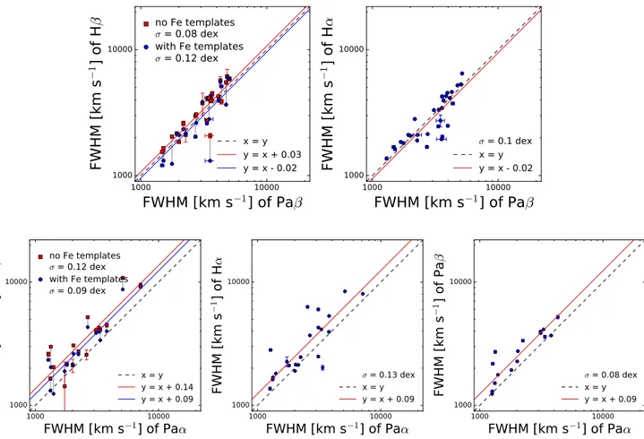
We compared the line widths of the broad components of Pa , Pa , H and H . Fig.3shows the comparison between the FWHM of
the broad Pa and H with or without tting Fe templates to the H region (e.g. Boroson & Green1992; Trakhtenbrot & Netzer2012). We tted the data using a linear relation with xed slope of 1 and we searched for the best intercept value. We equally weight each data point in the line t because the measured uncertainties from statistical noise are small (<5 per cent). For the FWHM of the broad Pa and H with Fe tting, we found the best t to have an offset of 0.029 – 0.003 dex with a scatter of = 0.08 dex. Without Fe tting, we nd a linear relation with an offset of 0.019 – 0.005 dex and a larger scatter ( = 0.13 dex). After taking into account the effect of the iron contamination on H , we did not nd a signi cant difference between the FWHM of H and the FWHM of Pa (the p-value of the Kolmogorov Smirnov test is 0.84). For the FHWM of Pa to H , we nd an offset of 0.023 – 0.03 dex and a scatter = 0.1 dex with no signi cant difference between their distributions (Kolmogorov Smirnov test p-value = 0.56).
We observed a trend for the mean FWHM of Pa to be smaller than the FWHM of the other lines. Comparing the FWHM of Pa and H we found the best t to have an offset of 0.092 – 0.005 dex with a scatter = 0.09 dex, while for the comparison between Pa and H , the offset is 0.094 – 0.006 dex with a scatter = 0.13 dex. For the comparison between Pa and Pa , the offset is 0.093 – 0.005 dex, with a scatter = 0.08 dex. Considering the mean values, we found that that the mean value of the FWHM of Pa (2710 – 294 km s 1) is smaller than the mean value of H and H (3495 – 436 and 3487 – 582 km s 1, respectively). For the sources with measurements of the broad components of both Pa and Pa , the mean value of the FWHM of Pa (2309 – 250 km s 1) is also smaller than the mean value of Pa (2841 – 283 km s 1). We note that none of these differences rises to the 3 level, so a larger sample would be required to study whether the FWHM of broad Pa is indeed smaller than the other lines.
We used the Anderson Darling and Kolmogorov Smirnov to further test if the distribution of the FWHM of Pa is signi cantly different from those of the other lines. We nd that both tests indicate that the populations are consistent with being drawn from the same intrinsic distribution at the greater than 20 per cent level for all broad lines. For the comparison of Pa with H , the Kolmogorov Smirnov test gives a p-value = 0.67, whereas for the comparison of Pa with H the p-value is 0.33 and for Pa with Pa the p-value is 0.63 suggesting no signi cant difference in the distributions of the FWHM of the broad components.
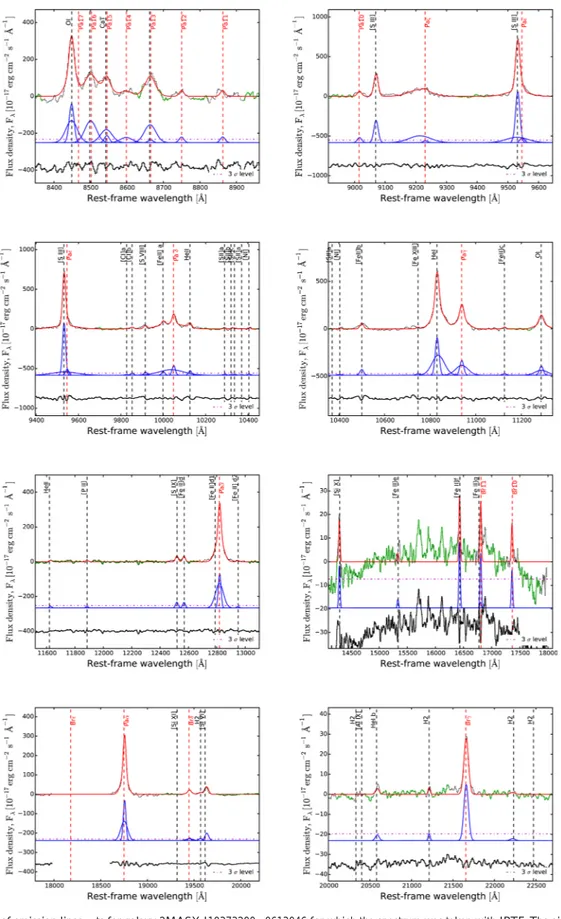
Figure 2. Example of emission lines ts for galaxy 2MASX J19373299 0613046 for which the spectrum was taken with IRTF. The eight panels show the emission lines ts for the regions (from the upper left to the bottom right): Pa14, Pa , Pa , Pa , Pa , Br10, Pa and Br . In the upper part of each gure, the spectrum is shown in black and the best t in red. The regions where the continuum is measured are shown in green. In the middle part of the gure, the components of the t are shown in blue and the magenta dashed line shows the threshold level for detection (S/N > 3). The lower part of the gure shows the residuals in black.
BASS IV: NIR spectroscopy
549
Figure 3. Upper panels: comparison between the FWHM of the broad components Pa and H (left). The red points show the FWHM of H measured without taking into account the iron contamination and the instrumental resolution and the blue points the FWHM of H measured using iron templates and corrected for the instrumental resolution. The black dashed line shows the one-to-one relation, the red and blue lines show the linear t with slope 1. The right-hand panel shows the comparison between the FWHM of the broad component of Pa and H . Lower panels: comparison of the FWHM of the broad components of Pa with H (left), H (middle) and Pa (right).
4.2 Hidden BLR
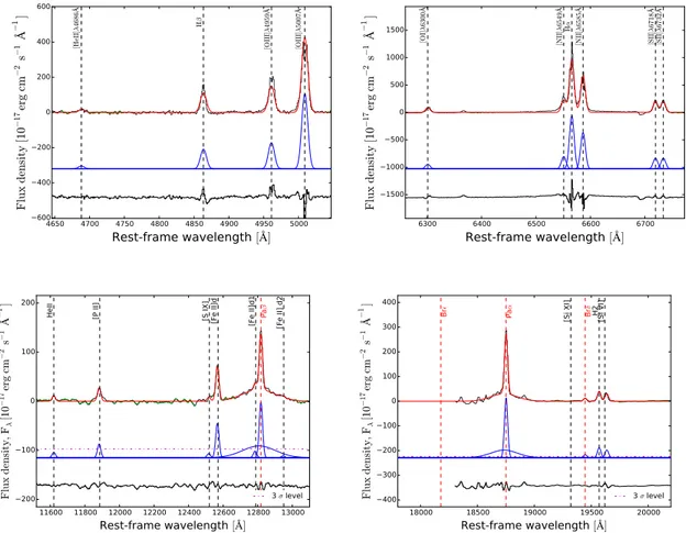
In our sample, there are 33 AGN classi ed as Seyfert 2 based on the lack of broad Balmer lines in the optical spectral regime. We found three of these (9 per cent) to show broad components (FWHM > 1200 km s 1) in either Pa and/or Pa . An example is shown in Fig.4. For Mrk 520 and NGC 5252, we detected the broad component of both Pa and Pa and also of HeI1.083 µm. For NGC 5231, we detected broad Pa , but the broad Pa component is undetected. For all three galaxies, we did not observe a broad component in the other Paschen lines. We do not detect a broad component in the Paschen lines for 16/33 (49 per cent) Seyfert 2 galaxies, in agreement with their optical measurements. For the remaining 14/33 (42 per cent) sources, we could not detect the broad components because the line is in a region with signi cant sky features.
We considered the values of NHmeasured by Ricci et al. (2015) and Ricci et al. (submitted). The Seyfert 2s in our sample have column densities in the range log NH = 21.3 25.1 cm 2 with a median of log NH= 23.3 cm 2. The three AGN showing a hidden BLR in the NIR belong to the bottom 11 percentile in log NH(Fig.5) among the Seyfert 2s in our sample (log NH< 22.4 cm 2).
Next, we considered the optically identi ed Seyfert 1 in our sample, and we investigated the presence of broad lines in their NIR spectra. In the Seyfert 1 1.5 in our sample, we did not nd spectra that lack the broad Pa or Pa component.
For the optical Seyfert 1.9 in our sample, the NIR spectra in general show broad lines except for some objects with weak optical broad lines. We found broad Paschen lines in 10/23 (44 per cent) Seyfert 1.9. For 6/23 (26 per cent) of Seyfert 1.9, the spectra do not cover the Pa and Pa regions. There are 7/23 Seyfert 1.9 (30 per cent) that do not show broad components in Pa and Pa . All these galaxies have log NH> 21.5 cm 2. Four of them have a weak broad component of H compared to the continuum (EQW[b H ] < 36 ¯). Further higher sensitivity studies are needed to test whether the broad H component is real or is a feature such as a blue wing.
4.3 Velocity dispersion
We measured the stellar velocity dispersion ( ) from the CaT region and from the CO band-heads in the H band and in the K band. The results are tabulated in Table8. Examples of tting are available in Appendix A2. In total, we could measure only for 10 per cent (10/102) of objects using the CaT region. The main reasons for this are as follows: lack of wavelength coverage of the CaT region, absorption lines too weak to be detected and presence of strong Paschen emission lines (Pa10 to Pa16) in the same wavelength of the CaT. We have a good measurement of for 31/102 (30 per cent) objects from the CO band-heads in the K band and for 54/102 (53 per cent) from the CO band-heads in the H band. We found that measured from the CaT region and from the CO band-heads (H MNRAS 467, 540 572 (2017)
Figure 4. Optical and NIR spectra of Mrk 520, which is an example of Seyfert 2 galaxy displaying a hidden BLR in the NIR. Upper panels: optical spectrum of the H and H region. The best t is in red, the model in blue and the residuals in black. Lower panels: NIR spectrum of the Pa and Pa region. In addition to the components explained above, the magenta dashed line in the middle part of the gures shows the detection threshold (S/N > 3) with respect to the tting continuum (blue).
Figure 5. Distribution of column density NHas a function of the FWHM of Pa . Blue points are Seyfert 1 which show a BLR in H , red squares are Seyfert 2 and violet stars are the Seyfert 2 with narrow lines in H that show a hidden BLR in the Pa . The dashed line shows the threshold NHvalue that separates optical Seyfert 1 and Seyfert 2 using the H line (Koss et al., submitted).
and K bands) are in good agreement (median difference 0.03 dex). However, we compared these measurements with literature values of measured in the optical and we found that the measured from the NIR absorption lines are 30 km s 1larger, on average,
than the measured in the optical range (median difference 0.09 dex). Further details about the comparison of measured in the different NIR spectral regions and in the optical is provided in Appendix A2.
4.4 Black hole masses
We derived the black holes masses from the velocity dispersion and from the broad Paschen lines. For the cases where we have both ,COand ,CaT, we use ,CO, since this method could be used for more sources with higher accuracy. We used the following relation from Kormendy & Ho (2013) to estimate the MBHfrom :
log MMBH = 4.38 log
200 km s 1 + 8.49 . (1)
This relation has an intrinsic scatter on log MBHof 0.29 – 0.03. There are different studies that derived prescriptions to estimate MBHfrom the broad Paschen lines (Pa or Pa ). All these methods use the FWHM of the Paschen lines Pa or Pa . Since Pa is near a region of atmospheric absorption, we have more measurements of the broad component of Pa ; therefore, we prefer to use this line to derive MBH. As an estimator of the radius of the BLR, previous stud-ies used the luminosity of the 1-µm continuum (Landt et al.2011a), the luminosity of broad Pa or Pa (Kim et al.2010, La Franca et al.2015) or the hard X-ray luminosity (La Franca et al.2015). We use the luminosity of broad Pa , since the continuum luminosity at
![Table 5. Relations of CLs ([Si VI ] and [S VIII ]) and [O III ] and [S III ] emission with the 14 195-keV emission and 2 10-keV emission.](https://thumb-eu.123doks.com/thumbv2/123dokorg/8094951.124740/8.892.111.773.106.645/table-relations-viii-iii-iii-emission-emission-emission.webp)
![Table 7. Relations of CLs and [S III ] luminosity with the 14 195-keV emission and 2 10-keV emission.](https://thumb-eu.123doks.com/thumbv2/123dokorg/8094951.124740/9.892.68.823.110.293/table-relations-cls-iii-luminosity-kev-emission-emission.webp)