A Mixed PDE-Monte Carlo Approach
for Pricing Credit Default Index Swaptions
Vlad Bally
∗, Lucia Caramellino
†and Antonino Zanette
‡Abstract
The problem of numerically pricing credit default index swaptions on a large number of names is considered. We place ourselves in a stochastic intensity framework, where Ornstein-Uhlenbeck type correlated processes are used to model both the firms distance to default and a macroeconomic state variable. The default of the firms follows here the reduced-form approach and the (random) intensity of the default depends on the behavior of the diffusion processes. We propose here a numerical method based on both a Monte Carlo and a deterministic approach for solving PDEs by finite difference. Numerical tests show the efficiency and the robustness of the proposed procedure.
2000 MSC: 91B28, 60H30, 65C05.
Keywords: credit default swaps and credit default swaptions; Feynman-Kac formula; Monte
Carlo methods; numerical approximation of PDEs solutions.
Acknowledgement. The authors are grateful to Darrell Duffie for having suggested the problem and for his encouraging help. The authors also thank the editor Marco Li Calzi and two anonymous referees for their useful comments and suggestions.
Corresponding author: Lucia Caramellino.
Address: Dipartimento di Matematica, Universit`a di Roma Tor Vergata, via della Ricerca Scientifica 1, I-00133 Roma, Italy.
Email: [email protected] Phone number: + 39 06 72594709 Fax number: + 39 06 72594699
∗Laboratoire d’Analyse et de Math´ematiques Appliqu´ees, Universit´e de Marne-la-Vall`ee, 77454
Champs-sur-Marne, France; e-mail: [email protected]
†Dipartimento di Matematica, Universit`a di Roma Tor Vergata, via della Ricerca Scientifica 1, I-00133 Roma,
Italy; e-mail: [email protected]
‡Dipartimento di Finanza dell’Impresa e dei Mercati Finanziari, Universit`a di Udine, Via Tomadini 30/A,
1
Introduction
The credit risk market has been growing rapidly in the last years. In particular, credit default swaps (CDSs) are one of the most actively traded credit derivatives (see e.g. Duffie [2], Duffie, Saita and Wang [4], Sch¨onbucher [9]).
A CDS provides protection in the event of default (called a credit event) of a specific company (called the reference entity). It is then an agreement between two counterparties, allowing the first one to be “long” a third-party credit risk, while the second counterparty to be “short” the credit risk. More precisely, one has first to introduce a reference asset, which is typically a credit risky bond issued by a third party corporation. Now, the two counterparties, say A and B, enter into an agreement: A pays to B a fixed periodic coupon for the specified life of the reference asset. Party B makes no payments unless the default event occurs for the reference asset. If such a credit event occurs, B makes a payment to party A, and the swap then terminates. The size of the payment is usually linked to the decline in the reference asset’s market value following the credit event.
In this paper, we consider the problem of pricing options on a portfolio of a large number of names (typically 100), where the underlying instrument for each name is a CDS. Such kind of risky financial instruments are known in the literature as index default swaptions or credit
default index swaptions, or also CDS index swaptions, the last one being the denomination we
will use all over this paper (see e.g. Jackson [6]).
A CDS index swaption is an option to buy or sell the underlying CDSs at a specified date. A payer swaption gives the holder of the option the right to buy protection (pay premium) and a receiver swaption gives the holder of the option the right to sell protection (receive premium). This basic definition of a CDS index swaption is similar to that of a CDS option, an option on a single-entity CDS, but a CDS index swaption is significantly different from a CDS option. In the case of an option on a single-entity, if the reference entity defaults before the options expiry, the option will be knocked out and becomes worthless. For a CDS index swaption, when a reference entity defaults before the options expiry, the loss will be paid by the protection seller to the protection buyer when the option is exercised. Even if there is only one entity in the portfolio, a CDS index swaption is still different from a single-entity CDS option: if the entity defaults before the options expiry, the options seller will pay to the protection buyer the lost amount at expiry. Clearly, a CDS index swaption is always more valuable than a single-entity CDS option.
In this paper, we allow the underlying possible defaults to follow an intensity-based model, in which the default time is a stopping time with a given intensity process (as in Duffie and Single-ton [5] or also Sch¨onbuncher [9]; different approaches are available in literature, see e.g. Jackson [6]). In our application, the default intensities depend on the firms distance to default and on some observable variable which is linked with the likelihood of default, such as a macroeconomic variable related to the business cycle. In our framework, both the firms distance to default and the macroeconomic variable are modelled through correlated Ornstein Uhlenbeck processes, with suitable coefficients. The model, which will be mathematically described later (Section 2), wad introduced firstly in Duffie and Wang [3] and in a second time it was generalized by Duffie, Saita and Wang [4].
swap-tions on a large number of names. It is based on a mixing between the classical numerical approximation by partial differential equations (PDEs) and the Monte Carlo approaches. For the model considered here, this algorithm offers a very efficient alternative to a pure vanilla Monte Carlo method, which is the classical tool to handle such kind of derivatives but, at the same time, becomes really unfeasible from a computational point of view when the number of the underlying firms is large. In fact, the comparisons with the results turning out by a pure vanilla Monte Carlo method are here presented mainly in order to benchmark the results of our algorithm. Let us add that it would be interesting to set up other pure and improved Monte Carlo techniques, such as control variates, which might possibly lead to better computa-tional efficiency. But, to our knowledge, no results are available in this direction at this stage, although this could be an interesting research problem.
The advantage of our algorithm is that it circumvents the nested simulation problem of a standard Monte Carlo algorithm by approximating conditional expectations using a PDEs approach. In fact, the PDEs approach is particulary suited to problems which are controlled by 2-dimensional diffusions, and can be efficiently handled by standard numerical techniques, such as finite differences. For the sake of clearness, it has to be remarked that the model we are going to use, and in particular the modelled correlations among the underlying stochastic processes, actually allows one to reduce to a number of different 2-dimensional problems equal to the number of the considered firms.
Finally, let us remark that even if the main goal of our work is to introduce a new methodology (the mixed PDE-Monte Carlo algorithm) constructed ad hoc for the pricing of a complex credit product (CDS index swaption), nevertheless we hope that this contribution helps to paving the road for future work addressing more challenging credit risk problems in high dimension in a dynamic setting.
The paper is organized as follows: in Section 2 we introduce the model of the stochastic intensity process for the default, a description of CDSs and CDS index swaptions; Section 3 is devoted to the presentation of the mixed PDE-Monte Carlo approach for pricing CDS index swaptions; numerical results are presented in Section 4.
2
The model
Let (Ω,F, {Ft}t,P) a filtered probability space, denoting the “risk neutral world”, where the
following (diffusion) processes are defined:
- (Yt)t∈[0,T ], modelled as
dYt = κY(θY − Yt)dt + σYdWtY; (1)
- as i = 1, . . . , n, (Di,t)t∈[0,T ], modelled as
dDi,t = κD(θD,i− Di,t)dt + σD(ρdWtc +
√
1− ρ2dWi
t). (2)
In (1) and (2), the processes WY, Wc, W1, . . . , Wn denote independent Brownian motions; ρ stands for a correlation coefficient, thus belonging to (−1, 1); κY, θY, σY and κD, θD,i, σD are
Notice that Y is independent of D1, . . . , Dn, while D1, . . . , Dn depend each other and such a
dependence is given by the correlation ρ. The referring filtration is then Ft= σ((WY
s , Wsc, Ws1, . . . , Wsn) ; s≤ t).
The intuitive meaning of the process Y arises in the fact that it models a macroeconomic state variable, i.e. the U.S. personal income growth, while D1, . . . , Dn model the firms distance to
default (for details, see Duffie and Wang [3] or Duffie, Saita and Wang [4]). Let us recall that the distances to default are correlated: in fact, the common Brownian motion Wc, which appears in all the SDEs giving D1, . . . , Dn (see (2)), captures the correlation amongst the individual
distances to default.
We suppose that the time of default follows here the intensity-based approach: setting τi as the
default instant for the ith firm, then its (random) failure intensity λi depends on both Y and Di as follows
λit= Λ(Yt, Di,t), where Λ(y, d) = exp(µ0+ µ1y + µ2d) (3)
Notice that the constant parameters µ0, µ1 and µ2 are common to all firms.
Let us recall that the above definitions mean that, for s < t, P(τi > t| Fs) = E(e−
∫t
sΛ(Yu,Di,u)du| Fs), on the set {τi > s},
where, from now on, the symbol E denotes the expectation under P.
For the construction of τi, we refer to Duffie and Singleton [5], Sch¨onbucher [9] or also Lando
[7]. We only recall here that this defines the default time as the first jump instant of a Cox process with intensity process λi, that is τ
i = inf{t ≥ 0 :
∫t
0λ
i
sds = Z}, being Z an exponential
random variable, of parameter 1, independent of all the Brownian motions already defined.
Remark 2.1 Let us make some remarks about our choice for the parameters modelling. Indeed,
concerning the distance to default processes, we have assumed a common mean reversion κD and a common volatility σD (see (2)); moreover, the intensity failures are defined through a function with common parameters, i.e. µ0, µ1 and µ2 (see (3)). Such kind of choice might appear very
restrictive, but this parsimonious model tries to overcome the problem of an extremely high-dimensional state-vector, consisting in one macroeconomic covariate, personal income growth Y , and the distance to default Di for each firm i among the n total ones. On the other hand, a relevant parameter concerning the distance to default, that is the long-run mean parameter θD,i (see (2)), varies firm by firm. Finally, the assumed homogeneity of correlation across different firms makes the model numerically tractable.
Let us now mathematically describe a CDS index swaption. This is an option to buy protection on the CDS index at rate K, which pays at time t
max (∑n
i=1 Vi,t, 0
)
where Vi,t is the market value at time t of a default swap on name i at rate K (notice that here K does not depend on i). Let us recall that a CDS is a credit derivative that protects its owner
So, if r denotes the risk free interest rate, the market value at time 0 of such an option is given by P0 = e−rtE ( max (∑n i=1 Vi,t, 0 )) . (4)
Let us now mathematically describe the quantities V1,t,.., Vn,t. Their values depend on the fact
that the default has or has not been observed at time t as follows:
- if τi ≤ t, that is name i has defaulted by time t, then Vi,t is the loss Li given default of name i:
Vi,t = Li;
- if τi > t, that is no default happened up to t, then Vi,t = Bi,t − Ai,t,
where Bi,t is the value at time t of the future payments by the seller of protection at
default and Ai,t is the value at time t of the future payments of the buyer of protection.
To give an explicit expression for Bi,t and Ai,t, one has to introduce further notations. Set t = t0 < t1 <· · · < tN = T the premium payment dates, which are such that tj+1− tj = ∆t for
any j (usually, ∆t is equal to 3 months). Define
pi,j,t =P(τi > tj|Ft) = E ( exp ( − ∫ tj t Λ(Ys, Di,s)ds) Ft ) (5) as the probability of survival from t to tj given Ft on{τi > t}. Finally, set
dj = exp(−r(tj − t)) as the time discount factor from time t to time tj. Then,
Bi,t =∑Nj=1dj(pi,j−1,t− pi,j,t)E(Li) Ai,t =
∑N
j=1djpi,j,tK.
(6)
To resume, for any i, the market value Vi,t at time t of a credit default swap on name i at rate K is given by
Vi,t = Li
1
{τi≤t}+ (Bi,t− Ai,t)1
{τi>t},where Bi,t and Ai,t are defined in (6).
Remark 2.2 In principle, the loss Li can be modelled in many different ways. Here, Li is a
random variable distributed between zero and one according to a specified law, which is the uniform one. It has to be said that more elaborate laws could be used in practice, but we should benchmark a simple case. It has been discussed allowing Li to be correlated with other
3
The mixed PDE-Monte Carlo numerical approach
Consider a derivative whose price P0 is given by (4). To numerically compute P0, consider a
Monte Carlo approach, that is
P0 = e−rtE ( max (∑n i=1 Vi,t, 0 )) ≃ e−rt M M ∑ m=1 max (∑n i=1 Vi,t(m), 0 )
where the index m stands for one of the total M trials and Vi,t(m) denotes the mth simulation for Vi,t. Then, the problem is how to simulate
Vi,t = Li
1
{τi≤t}+ (Bi,t− Ai,t)1
{τi>t}. (7)Obviously, the r.v. Vi,t cannot be exactly replicated, so we have to discuss firstly an
approxi-mation ¯Vi,t of Vi,t.
3.1
Checking if default does or does not occur
First of all, we have to check if the default of the ith firm does or does not occur up to time
t. In order to do this, we have to use the default probabilities, which of course depend on
the paths followed by the process Y and Di on [0, t]. Therefore, one has first to discretize the
time interval [0, t] in order to set up an Euler scheme for the two processes and consequently to compute the default probabilities. To be more precise, set 0 = s0 < s1 < · · · < sℓ = t a
discretization of [0, t] such that sk+1− sk = ∆s is “small enough”. Let us define ¯Y and ¯Di,t the
(discrete) Euler schemes for Y and Di respectively:
¯
Y0 = Y0, ¯Di,0 = Di,0 and for k = 1, . . . , ℓ :
¯
Yk= ¯Yk−1+ κY(θY − ¯Yk−1)∆s + σY∆WkY
¯
Di,k = ¯Di,k−1+ κD(θD,i− Di,k−1)∆s + σD(ρ∆Wkc+
√
1− ρ2∆Wi k).
Here, ∆WkY, ∆Wkc and ∆Wki denote the variation between sk−1 and sk of the Brownian motions WY, Wc and Wi respectively. Let us stress that, in our notations, one has ¯Y
k ≃ Ysk and
¯
Di,k ≃ Di,sk. Once the above schemes are set, we can approximate the event “the default has
occurred up to time t” as follows. First, let us observe that the probability of no default of the firm i up to sk given that the firm is still alive at time sk−1 can be approximated by using the
approximation ( ¯Y , ¯Di) as follows: on the set{τi > sk−1} one has
P(τi > sk| Fsk−1) =E ( e− ∫sk sk−1Λ(Ys,Di,s)ds Fsk−1 ) ≃ e−Λ( ¯Yk−1, ¯Di,k−1)∆s. Then, if we set ¯ qi,k = e−Λ( ¯Yk−1, ¯Di,k−1)∆s,
- one first computes ¯qi,0 and: with probability ¯qi,0 one says that no default occurred up to s1;
- if the default did not occurred up to sk−1, then one computes ¯qi,k and: with probability ¯qi,k
one says that no default occurred up to sk; with probability 1− ¯qi,k one says that default
did occur up to sk.
Let us recall that in practice this means to generate r.v.’s Zi,k, uniformly distributed on (0, 1),
independent each other and of any other random variable written above, and to check if Zi,k is
or is not less than ¯qi,k: if Zi,k < ¯qi,k then no default is assumed to occur; if Zi,k > ¯qi,k then the
default is assumed to occur.
This procedure brings to an approximation ¯
1
i of the random variable1
{τi>t}: we set ¯1
i = 1 ifno default has been observed up to sℓ = t, otherwise ¯
1
i = 0. Once ¯1
i is obtained, we set:- Vi,t ≃ ¯Vi,t = Li if ¯
1
i = 0;- Vi,t ≃ ¯Vi,t = (B− A)i,t if ¯
1
i = 1,where (B− A)i,t is a suitable approximation for Bi,t− Ai,t, to be discussed in Section 3.2 and
3.3.
3.2
Standard Monte Carlo approach if default does not occur
In this Section, we suppose to have observed no default up to t, that is to be on the set{τi > t}.
Then, we have to approximate Bi,t − Ai,t. By formula (6), we can rewrite Bi,t− Ai,t =
∑N
j=1dj(pi,j−1,t− pi,j,t)E(Li)−
∑N
j=1djpi,j,tK
= ∑Nj=1ci,jpi,j,t+ ci,0
(8) where ci,j = E(Li)d1 if j = 0 −(K + E(Li))dj +E(Li)dj+1 if 1≤ j ≤ N − 1 −(K + E(Li))dN if j = N (9)
(we have used above the notation pi,0,t = 1).
This means that Bi,t− Ai,t is a linear combination of the functions pi,j,t =E ( exp ( − ∫ tj t Λ(Ys, Di,s)ds) Ft ) .
Now, since the pair (Xi,s)s = (Ys, Di,s)s is a diffusion, then the Markov property holds, so that pi,j,t = Pi,j(t, Xi,t), where Pi,j(t, x) = Et,x
( exp ( − ∫ tj t Λ(Xi,s)ds )) , (10) where as usual Et,x denotes expectation among the paths starting at x at time t. Therefore, pi,j,t has a representation in terms of an expectation, so that one can think to compute it by the
standard Monte Carlo method: setting ¯Xi,t = ( ¯Yt, ¯Di,t) the approximation already observed for
Xi,t, then
pi,j,t ≃ Pi,j(t, ¯Xi,t)≃
1 M′ M′ ∑ m′=1 exp ( − ∫ tj t Λ( ¯Xi,s(m′))ds ) (11)
where ( ¯Xi,s(m′))s≥t denotes a simulation of an approximation ( ¯Xi,s)s≥t (e.g. by Euler scheme) for
(Xi,s)s≥t on the time interval [t, T ] starting from ¯Xi,t at time t (and obviously, the integral is
approximated by Riemann sums).
Therefore, summing up, we have for any firm i:
- m = 1, . . . , M simulations of the path on [0, t], telling us if default does or does not occur,
and if not, giving us a position, say ¯Xi,t(m), of the pair (Y, Di) at time t;
- for any m = 1, . . . , M giving no default, we have to start with M′ more simulations of the pair Xi = (Y, Di) on [t, T ] starting at ¯X
(m)
i,t , in order to approximate the probabilities as
in (11).
This can give rise to M × M′ simulations, for any i = 1, . . . , n, so the total number can arrive to M × M′ × n. In other words, an algorithm of this kind is too expensive from a computational point of view. One could think to use some variance reduction techniques, for example a control variate. But this approach would not overcome the problem of the further
M′ simulations, leading us to look for an alternative method.
3.3
PDE approach if default does not occur
The idea starts from the fact that deterministic methods to approximate expectations by nu-merical solutions of PDEs, work quite well if the dimension is small.
Let us come back to Bi,t− Ai,t and let us rewrite it as
Bi,t − Ai,t = φi(t, Xi,t) (12)
where (see (8), (9) and (10))
φi(t, x) = N
∑
j=1
ci,jPi,j(t, x) + ci,0. (13)
Now, we propose here to numerically compute φi(t, Xi,t) as the solution of a parabolic PDE
on R2, which in turn is evaluated by finite difference methods. To this purpose, using the
Feynman-Kac formula one can first compute Pi,j(t, Xi,t) as follows:
Proposition 3.1 One has Pi,j(t, Xi,t) = vi,j(t, Xi,t′ ), where Xi,t′ = (Yt′, Di,t′ ) is the 2-dimensional diffusion solving the SDE
dYt′ =−κYYt′dt + σYdWtY, Y0′ = Y0
dDi,t′ =−κDD′i,tdt + σD(ρdWtc+√1− ρ2dWi
t), D′i,0 = Di,0.
(14)
and vi,j solves
∂tvi,j(s, x) +Lvi,j(s, x)− gi(s, x)vi,j(s, x) = 0 (s, x)∈ (0, tj)× R2 vi,j(tj, x) = 1
being (recall that x = (y, d)) L = 1 2σ 2 Y∂yy2 + 1 2σ 2 D∂dd2 − κYy∂y− κDd∂d, gi(s, x) = qi(s) exp(µ1y + µ2d), with qi(s) = exp ( µ0+ µ1θY(1− e−sκY) + µ2θD,i(1− e−sκD) )
Remark 3.2 There exists a very simple relation connecting the processes Xi = (Y, Di) and Xi′ = (Y′, Di′): for any s,
Ys′ = Ys− θY(1− e−κYs) and D′i,s= Di,s− θD,i(1− e−κDs).
The proof is straightforward (but see also the next proof).
Proof of Proposition 3.1. It is well known that the pair (Xi,s)s= ((Ys, Di,s))shas an explicit
expression given by Ys = Y0e−κYs+ θY(1− e−κYs) + σY ∫s 0 e−κ Y(u−s)dWY u Di,s= Di,0e−κDs+ θD,i(1− e−κDs)+
+σD ∫s 0 e−κ D(u−s)d(ρWc u + √ 1− ρ2dWi u)
Then, setting Ys′ = Ys− θY(1− e−κYs) and D′i,s= Di,s− θD,i(1− e−κDs), it is straightforward
to see that the pair (Xi,s′ )s = ((Ys′, D′i,s))s solves (14). Now, for any s,
Λ(Ys, Di,s) = exp
( µ0+ µ1Ys+ µ2Di,s ) = exp ( µ1Ys′+ µ2Di,s′ ) · qi(s) where qi(s) = exp ( µ0+ µ1θY(1− e−sκY) + µ2θD,i(1− e−sκD) )
Then, for x = (y, d), if gi(s, x) = qi(s) exp(µ1y + µ2d), one has Λ(Xi,s) = gi(s, Xi,s′ ) and
therefore, Et,Xi,t ( exp ( − ∫ tj t Λ(Xi,s)ds )) =Et,Xi,t′ ( exp ( − ∫ tj t gi(s, Xi,s′ )ds )) .
In other words, we have Pi,j(t, Xi,t) = vi,j(t, Xi,t′ ), where we have put vi,j(t, x) = Et,x ( exp ( − ∫ tj t gi(s, Xi,s′ )ds ) .
Now, by the Feynman-Kac formula, it immediately follows that vi,j solves the PDE problem
(15). 2
Using Proposition 3.1, one can represent the function φi in (12) and (13) as the solution of a
PDE problem, as follows.
Proposition 3.3 Consider the following backward set of functions ψi,N(s, x), . . . , ψi,1(s, x) (recall that L and gi are defined in Proposition 3.1):
- ψi,N(s, x) solves:
∂tψi,N(s, x) +Lψi,N(s, x)− gi(s, x)ψi,N(s, x) = 0 (s, x)∈ (0, tN)× R2 ψi,N(tN, x) = ci,N;
- as j = N − 1, . . . , 1, ψi,j(s, x) solves:
∂tψi,j(s, x) +Lψi,j(s, x)− gi(s, x)ψi,j(s, x) = 0 (s, x)∈ (0, tj)× R2 ψi,j(tj, x) = ci,j+ ψi,j+1(tj, x)
Then, φi(t, Xi,t) = ψi,1(t, Xi,t′ ) +E(Li)d1, where X′ is defined through (14).
Proof. Consider first ψi,N: it solves the same PDE as in (15) with j = N , with constant (final)
Cauchy condition equal to ci,N. Then, it holds
ψi,N(s, x) = ci,Nvi,N(s, x), s≤ tN.
Now, for j = N − 1, . . . , 1, again ψi,j solves the same PDE as in (15), with (final) Cauchy condition equal to ci,j + ψi,j+1(tj, x). It then follows that
ψi,j(s, x) = ci,jvi,j(s, x) + ψi,j+1(s, x), s≤ tj.
Therefore, by iteration, ψi,1(s, x) = N ∑ j=1 ci,jvi,j(s, x), s≤ t1,
so that as s = t(< t1) one has
ψi,1(t, Xi,t′ ) = N
∑
j=1
ci,jvi,j(t, Xi,t′ ) = N
∑
j=1
ci,jPi,j(t, Xi,t),
the last equality being proved in Proposition 3.1. Therefore, by (13), one has
φi(t, Xt) = ψi,1(t, Xi,t′ ) + ci,0 = ψi,1(t, Xi,t′ ) +E(Li)d1,
and the statement holds. 2
Remark 3.4 Let us observe that one could also avoid considering the new process Xi′ and use directly the original process Xi. In such a case, one would obtain quite the same results, but of
course the operator ∂t+L − gi has to be replaced by ∂t+Li− Λ. It has to be stressed that the
advantage of our representation is that the differential operator L is the same for any i and only gi changes as i varies. Now, this is important from a computational point of view since
this allows to reduce the number of numerical operations (e.g. in an explicit finite differences scheme).
Now, the result in Proposition 3.3 is used in practice in the following way. We first compute an approximation ¯φi of φi by using deterministic numerical methods for solutions of PDEs (here,
for a fixed (firm) i, the associated PDE is on R2, so deterministic methods efficiently work).
Therefore, we can finally set the approximation
Bi,t− Ai,t ≃ (B − A)i,t = ¯φi(t, ¯Xi,t).
The algorithm can be resumed as:
a) fix the firm i and the mth simulation (i = 1, . . . , n and m = 1, . . . , M );
b) following Section 3.1, check if default does or does not occur on [0, t], and set the mth simulation ¯Vi,t(m) of Vi,t as:
b1) if default is observed, then ¯Vi,t(m)= Li;
b2) if no default is observed, then ¯Vi,t(m) = ¯φi(t, ¯X
(m)
i,t )
c) compute the price by averaging:
P0 ≃ ¯P0 = e−rt M M ∑ m=1 max (∑n i=1 ¯ Vi,t(m), 0 )
It is worth to stress some remarks concerning item b2) above.
We numerically solve the PDEs in Proposition 3.3 for each name i with a finite difference method. The numerical procedure consists in the following five steps.
1. The set of linear parabolic problems in Proposition 3.3 have to be localized to a bounded domain in space, that isR2 is in practice replaced by Ω
l = (ymin′ , ymax′ )×(d′min, d′max). The
choice of Ωl must answer two main purposes. First, Ωl must be large enough to ensure
the convergence of the approximating function to the true one. Second, the values of ( ¯Yt′(m), ¯D′(m)i,t )m (obtained from ( ¯Y
(m)
t , ¯D
(m)
i,t )m by using the transformation as in Remark
3.2) have to be contained in Ωl. Then, for each name i, we first simulate all the paths
and secondly construct the grid. Afterwards, we solve the PDEs with a finite difference method.
2. The approximating solutions ¯ψi,N, . . . , ¯ψi,1 are computed by means of finite difference
methods involving discrete functions. For our numerical studies, we use an explicit finite difference method (see Wilmott, Dewynne and Howison [10], Villeneuve and Zanette [11]) and we suitably add, as usually done, Neumann homogenous artificial boundary conditions.
3. We construct for this purpose a time-space grid. Each time interval (tj−1, tj] is split
in subintervals and we consider a mesh of the space domain [ymin′ , ymax′ ]× [d′min, d′max] consisting of subintervals (yk′, yk+1′ ) and (d′k, d′k+1), where ymin′ = y0′ < . . . < y′MY = ymax′ and d′min = d′0 < . . . < d′M
D = d
′
4. Since we need ¯φi at time t, we solve backwardly the PDEs in Proposition 3.3 up to t, so we will have (see Remark 3.2)
¯ φi(t, yj1, dj2) = ¯ψi,1(t, y′j1, d ′ j2) +E(Li)d1, with y′j1 = yj1 − θY(1− e−κ Yt) and d′ j2 = dj2 − θD,i(1− e−κ Dt)
5. Now, in order to estimate ¯φi(t, ¯Y
(m)
t , ¯D
(m)
i,t ), we look for the four points of the space grid
which are neighborhood points for ( ¯Yt′(m), ¯Di,t′(m)) and then we approximate ¯φi(t, ¯Y
(m)
t , ¯D
(m)
i,t )
using bilinear interpolation of ¯ψi,1 in these points.
Remark 3.5 Let us recall that the use of PDEs techniques have been done in order to
over-come the problem of the further nested M′ simulations for each firm i. This problem could be handled also by using regression in place of PDEs, as it has been done for numerically pricing American options (see Carriere [1] and Longstaff and Schwartz [8]), a topic which is worthy to be investigated. However, the use of regression for approximating conditional expectations is a very good idea for American option pricing purposes, where the time interval is split into small time subintervals. In fact, this ensures that the conditional expectations is done following the law of a process in a small time interval, and this makes the regression approximation work very well. Our context is actually different (see e.g. (10)), so that a method involving regression is not trivial and should be analyzed in detail.
4
Numerical results
In this Section we numerically illustrate the efficiency of the PDE-Monte Carlo approach intro-duced in Section 3.3 and we compare, for benchmark purposes, this approach with the vanilla Monte Carlo approach of Section 3.2. All the computations have been performed in double precision on a PC Pentium 1.73 GHz.
We treat the problem of pricing CDS index swaptions in the model introduced in Section 2 and we consider the following values of the parameters :
• varying number of firms: n = 50, 100, 125;
• option parameters: times t = 1, T = 6 then tj = t + 0.25 j, j = 1, . . . , 20; Li uniformly
distributed on (0, 1); interest rate r = 0.05; rate K = 0.001;
• default probability parameters: µ0 =−4.2017, µ1 =−0.4597, µ2 =−0.4411
Concerning the diffusion parameters, we consider two test cases, named A and B :
• case A: κY = 0.6524, θY = 1.8901, σY = 0.8888, Y0 = 3; κD = 0.1185, θD,i= 4.32 + i/n, σD = 0.9657, Di,0 = 3; correlation coefficient ρ = 0.2684;
• case B: κY = 0.1137, θY = 0.1076, σY = 1, Y0 = 3; κD = 0.0355, θD,i = 4.32 + i/n, σD = 0.346, Di,0 = 3; correlation coefficient ρ = 0.2684;
The choice of these parameters was inspired by a similar combination in Duffie and Wang [3]. We are going to compare the results obtained by the mixed PDE-Monte Carlo approach and the (standard) Monte Carlo algorithm, in which the following settings are taken into account. (i) As for the mixed PDE-Monte Carlo approach, we take the number of simulation M = 10.000, the number of discretization step ℓ = 32 in which the time interval [0, t] is split. The PDEs are numerically solved through an explicit finite difference method, with time discretization step set equal to 40, while the spatial discretization step is obtained via the stability condition. We add Neumann homogenous artificial boundary conditions.
(ii) As for the Monte Carlo algorithm, we take a number of simulations M of the first part equal to the number of simulations M′ of the second part, both equal to 1000 or 10000; moreover, we split the time interval [0, t] in ℓ = 32 or 64 subintervals.
The results for the price and the estimated standard deviation, divided by the square root of the number of simulations, for case A and B are presented in next tables, in Price and St.Dev./√M
column respectively, according to the mixed PDE-Monte Carlo method summarized in (i) (in tables, PDE-MC) or the vanilla Monte Carlo method as in (ii) (in table, MC 1000× 32 and MC 10000× 64). Finally, reports are given in Table 1, 2 and 3, for a number n of firms equal to 50, 100 and 125 respectively.
CASE A B
Price St.Dev./√M Price St.Dev./√M
PDE-MC 0.038 0.002 0.094 0.003
MC 1000× 32 0.036 0.005 0.082 0.010
MC 10000× 64 0.036 0.001 0.095 0.003
Table 1: Number of firms n = 50: price and standard deviation for the mixed PDE-Monte Carlo method (PDE-MC) and the full Monte Carlo one (MC).
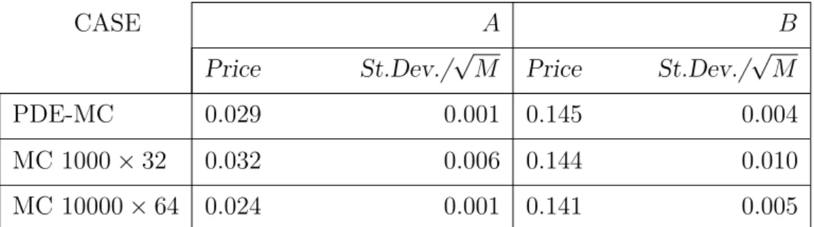
CASE A B
Price St.Dev./√M Price St.Dev./√M
PDE-MC 0.029 0.001 0.145 0.004
MC 1000× 32 0.032 0.006 0.144 0.010
MC 10000× 64 0.024 0.001 0.141 0.005
Table 2: Number of firms n = 100: price and standard deviation for the mixed PDE-Monte Carlo method (PDE-MC) and the full Monte Carlo one (MC).
CASE A B Price St.Dev./√M Price St.Dev./√M
PDE-MC 0.024 0.001 0.166 0.006
MC 1000× 32 0.021 0.006 0.162 0.020
MC 10000× 64 0.021 0.001 0.170 0.007
Table 3: Number of firms n = 125: price and standard deviation for the mixed PDE-Monte Carlo method (PDE-MC) and the full Monte Carlo one (MC).
Let us take the price turning out by the MC 10000× 64 as a benchmark value. In such a case, we observe two different performances for our PDE-MC method. In fact, case B works very well, because the relative error is between 1% and 2.8%. Despite this, case A works poorer, giving an error higher than the one arising from case B. Nevertheless, it has to be remarked that in case A prices are much smaller, and it is well known that low values might be responsible of high relative errors.
Let us spend some final words about the computational cost in time of the PDE-MC algorithm. The time computation results for n = 50, 100, 125 are presented in next Table 4.
number of firms n = 50 n = 100 n = 125
PDE-MC CPU time 10 sec. 19 sec. 23 sec.
Table 4: Time computation for the mixed PDE-Monte Carlo method (PDE-MC).
Obviously, comparisons with the time needed by the full Monte Carlo algorithms are not sig-nificant (just to give an idea, the range is in the between of some hours and some days, and in fact the use of the vanilla Monte Carlo approach has been done in order to benchmark our results). However, Table 4 shows very low CPU times spent by our algorithm. We can then conclude that the proposed mixed PDE-Monte Carlo method can be used to provide a fast and reasonably robust pricing of CDS index swaptions.
5
Conclusions
In this paper, we have investigated a new numerical method, a mixed PDE-Monte Carlo algo-rithm, to approximate the price of credit default index swaptions on a large number of names in presence of stochastic intensity.
The straightforward application of a pure Monte Carlo algorithm is too expensive from a computational of view. On the contrary, the main appeal of the proposed methodology is that it allows to obtain price results for this credit derivatives product with a cheap computational time cost. The numerical results confirm also the reliability of the method.
Based on these results, the mixed PDE-Monte Carlo algorithm presented in this work may be considered to tackle our credit derivative pricing problems in a dynamic setting.
References
[1] J.Carriere: Valuing of the early-exercise price for options using simulations and non para-metric regression. Insurance:Mathematcs and Economics, 14, 19-30, 2001.
[2] D. Duffie: Credit Swap Valuation. Financial Analusts Journal, January-February ,73-87, 1999
[3] D. Duffie and K. Wang: Multi-Period Corporate Failure Prediction with Stochastic Co-variates. Preprint, 2004.
[4] D. Duffie, L. Saita and K. Wang: Multi-Period Corporate Failure Prediction with Stochas-tic Covariates. Preprint available at www.standford.edu/∼duffie/ddkw.pdf (last check: May 3, 2006).
[5] D. Duffie and K. Singleton: Modelling Term Structures of Defaultable Bonds. Review of
Financial Studies, 12, 687-720, 1999.
[6] A. Jackson: A New Method for Pricing Index Default Swaptions. Working paper, Citi-group, 2005.
[7] D. Lando: On Cox Proceses and Credit-Risky Securities. Review of Derivatives Research,
2, 99-120, 1999.
[8] F. Longstaff and E. Schartz: Valuing American Options by Simulations: a Simple Least-Squares Approach. Reviews of Financial Studies, 14, 19-30, 2001.
[9] P.J. Sch¨onbucher: Credit Derivatives Pricing Models: Models, Pricing, Implementation. Wiley Finance, 2003.
[10] P. Wilmott, J. Dewynne and S. Howison: Option Pricing: Mathematical Models and
Com-putation Oxford Financial Press, 1993.
[11] S. Villeneuve and A. Zanette: Comparison of Finite Difference Methods for Pricing Amer-ican Options on Two Stocks. Working paper of the Dipartimento di Finanza dell’Impresa e dei Mercati Finanziari, Universit`a di Udine, 1-2001