A revision of the revaluation index of Spanish pensions

DOI: 10.7866/HPE-RPE.17.3.5

A Revision of the Revaluation Index of Spanish Pensions

This article reviews the methodological aspects of the revaluation index of Spanish pensions developed following Law 23/2013 which regulates the sustainability factor and revaluation index of the Social Security pension system. From a gradual breakdown of the elements that make up the revaluation index, an exposition is given of the formal and implementation problems it involves. Finally, an alterna­ tive model based on dynamic optimization techniques is proposed and its use is illustrated with nu­ merical examples.

Keywords: Revaluation index, automatic balancing mechanisms, Spanish Social Security System. JEL Classification: H55, J26

1. Introduction

Over the last fifteen years, many European countries have believed a profound reform of their state pension system to be necessary [Börsch-Supan (2012)]. Strong demographic pres­ sure, an acute economic crisis and internal imbalances have affected the sustainability of state pension systems. Among the measures taken, we would highlight the parametric changes in the system, i.e., those changes that affect one or several variables without affecting their structure. Examples are raising the retirement age or increasing the number of years in employment used to compute the base pension. Also, in some cases the reforms have involved the incorporation of a sustainability factor so as to automatically modify certain aspects of the pension system.

The sustainability factors fall within the category of so-called “automatic balancing mechanisms”. The underlying idea is to link one or more parameters of the system with the evolution of an exogenous variable. This may be life expectancy, the variation of the ratio of pensioners to contributors, or GDP growth (see Diamond, 2004; Sakamoto, 2008 or Vidal

Meliá et al. 2009). Its purpose is to re-establish the financial equilibrium of the system without requiring legislative intervention any time an adjustment is needed. In this way, the political risk is reduced while taking unpopular reforms. A comprehensive discussion of this topic can be found in Turner (2009), reviewing the experience of several countries adopting automatic balancing mechanisms.

Automatic balancing mechanisms may vary depending on several factors (as the frequen­ cy of adjustment) and can be structured in many different ways. One popular mechanism is to index benefits to improvements in life expectancy. This is the case of Portugal and Finland, where the base pension is reduced according to increases in this variable. In the case of Portu­ gal the reduction is proportional to the percentage change in life expectancy, whereas in Fin­ land it is done reducing monthly benefits actuarially to reflect longer life. Similarly, some systems has opted to index retirement age to life expectancy. This is the path taken in Denmark, indexing public old-age pensions as of 2030. Also in Finland, as of 2027, the eligibility age for old-age retirement will be linked to life expectancy. Another alternative is indexing the number of years required for a full benefit. In France, e.g., the number of contribution years increases with the life expectancy so that the ratio of the number of contribution years to the number of years spent in pension keeps constant.

Automatic balancing mechanisms can grow in complexity incorporating economic vari­ ables to determine the revaluation of pensions. In Germany, for example, the revaluation of the pensions is affected by changes in gross income and the variation of the ratio between pension­ ers and contributors (Börsch-Supan et al., 2003). In Japan, the revaluation depends on prices, life expectancy and a dependency ratio. In Netherlands, Denmark, Finland and Norway the revaluation is linked to variations in wages. The case of Sweden is more complex as the auto­ matic balancing mechanism is based on the result of the actuarial balance of the system [Set­ tergren (2001)]. A similar approach was followed by Japan (Sakamoto, 2005) and Canada (Canada Pension Plan, 2007).

In the Spanish case, with the progressive aging of the population, the problems that the state pension system is facing are no different from those affecting most European countries. According to the demographic projections included in “The 2015 Ageing Re­ port” (European Commission, 2015), it is estimated that the 9 million pensioners in 2013 will become 15.7 million in 2050, with an old-age dependency ratio1 _{raising from 26.8}

in 2013 to 62.3 in 2050. Also, the long-term demographic projections of the National Statistics Institute 2013-2063 estimate that life expectancy at the age of 65 is increasing by about nineteen months every ten years. Thus the projections indicate that the system will have to provide pensions to more beneficiaries for longer time. On the other hand, birth rates are decreasing. The rate of growth of revenue from contributions is therefore slowing. According to the same European Commission’s projections, the ratio of con­ tributors to pensioners will fall from 1.91 in 2015 to 1.2 in 2050. For these reasons, in recent years several studies have highlighted the need to implement reforms in the sys­ tem (see for example Conde-Ruiz and Alonso, 2004; Jimeno et al., 2008; Díaz-Giménez and Díaz-Saavedra, 2009; Sánchez-Martín, 2010).

Following the recent trends in pension reforms, the Spanish Government also opted in favor of an automatic mechanism in order to deal with the system imbalances through the ap­ proval of Law 23/2013 regulating the Sustainability Factor and the Revaluation Index of the Social Security Pension System. Such reform aims to adjust the initial pension according to variations of life expectancy (sustainability factor) and replaces the previous linkage between pension revaluation and the Consumer Price Index (CPI) for a revaluation method based on an economic model designed to guarantee the financial stability of the system (revaluation index). Although the introduction of the sustainability factor did not pose any controversial issues, it was not the case of the model employed for deriving the revaluation index. The complexity of the methodology used to revaluate the pensions and its lack of definition in certain aspects has originated a series of papers dealing with the recent reform. An early allusion to the prob­ lems of the revaluation index is De las Heras et al. (2014). Sánchez-Martín (2014) makes use of the revaluation index while exhaustively simulates the future performance of the Spanish pension system after the 2013 reform, but without much detail about how the revaluation index is applied. Devesa et al. (2015) study the impact of the revaluation index under different eco­ nomic scenarios, and discusses some of its technical aspects. Our approach differs from the last two in that we do not aim to assess the economic implications of the reforms. Instead, we aim to study the model from an analytical perspective, presenting a major in-depth analysis of the economic model underlying the derivation of the revaluation index.

Two references closer to our approach are AIReF (2014), which largely discusses the ap­ plication of the revaluation to real data, and Moral-Arce and Geli (2015), that study the prob­ lem of circularity existent in the revaluation formula. Our study expands and complements these works. After an extensive description of the actual model and its legislative antecedents, we present new results on the inner inconsistency of the revaluation formula as approved by Law and propose solutions to its inaccuracies. We obtain partial results on the evolution of the financial result of the pension system. In particular, we study the convergence between reve­ nues and expenditures and extend the model for the case that previous debt needs to be ab­ sorbed thought the revaluation mechanism. Also, close form solutions are obtained for particu­ lar cases. Finally, we propose an alternative model for pension revaluation based on dynamic optimization techniques, tailored to this particular problem, that mimics the characteristics of the current law and compare its performance with some numerical examples.

The paper is written having mind the potential interest of researchers and policymakers in the recent trend of adoption of automatic balancing mechanisms. We believe that is crucial that existing models are easily accessible and well understood so that policymakers can potentially take them into account in their reforms and implement (partially or totally) adequate ideas they might contain. We approach our analysis decomposing the formula in its basics components and gradually incorporating new elements to study its impact in the final formulation.

The present paper has the following structure. Section 2 describes the previous revaluation model and the current pension reform. Section 3 analyses the mathematical aspects and formu­ las of the model, highlighting the drawbacks with their formalization and implementation. In

Section 4, we shall discuss some extensions of the basic model. Section 5 compares the actual revaluation model with an alternative model based on a classical dynamic programming ap­ proach. Numerical examples with real data are provided in Section 6. Finally, Section 7 pres­ ents our conclusions.

2. The revaluation of Spanish pensions

As was mentioned in the previous section, one of the objectives of the reform provided in the Law 23/2013 is to rethink the revaluation model of the state pensions, by means of a new modification of the revised General Law on Social Security. In particular this would modify the pension revaluation scheme in the Social Security system. In this section we shall provide an historical overview of the legislative antecedents of the revaluation method of Spanish pensions and the recent reform. We believe that a comprehensive description will help to understand the approach finally chosen to reform the pension system in Spain.

2.1. Legislative antecedents on pension revaluation

The legislative antecedents to the new reform established a direct link between the CPI and the revaluation of the pensions. Law 24/1972 of 21 June foresaw in its Article 5 a periodic re­ valuation of the pensions by the Government. This was proposed by the Labour Minister, tak­ ing into consideration among other indicative factors the mean rise in wage levels, the cost of living index, and the general evolution of the economy, as well as the economic possibilities of the Social Security system. This procedure was also reflected in the revised General Law on Social Security of 20 June 1976 in its Article 92.

Subsequently, Law 26/1985 of 31 July, established in its Article 4 that pensions based on the application of the modifications made to this law would be revalued at the beginning of each year in accordance with the projected CPI for that year. These considerations were re­ flected in the law Royal Decree-Law 1/1994 of 20 June approving the revised General Law on Social Security, which includes in its Article 48 the revaluation of the pensions because of re­ tirement and disability in agreement with the projected CPI for that year.

The pre-reform pension revaluation model, effective beginning with the passage of Law 24/1997 of 15 July, established an automatic revaluation of the pensions in accordance to the annual variation of prices, thus ensuring the purchasing power of the pensioners. The mecha­ nism which determined the revaluation of the contributory pensions (including the amount of the minimum pension) was as follows. First, at the beginning of each year, the pensions were revalued in accordance with the projected CPI for that year. Second, if the CPI accumulated between the previous November and the November of the financial year corresponding to the revaluation was greater than projected, then the revaluation was adjusted by that difference.

This adjustment was paid in a single payment before April 1 of the subsequent year. In the case that the CPI between the two Novembers was less than expected, the difference was to be ab­ sorbed in the revaluation of the following financial year.

The automatic revaluation mechanism introduced in the Law 24/1997 was not, however, always applied. This was due to the need to comply with certain fiscal objectives. The revalu­ ation of the pensions corresponding to 2011 was suspended by the Law 39/2010 of 22 Decem­ ber of the General State Budget. Although it was not applied to the Social Security’s minimum pensions, non-contributory pensions, or the (now extinct) non-recurring Compulsory Elderly and Incapacity Insurance pensions, the extraordinary suspension of the pensions marked a break in the guarantee to maintain their real value.

For 2012, due to the large deficit in the Social Security system and the liquidity tensions at the end of the year corresponding to the ordinary and extraordinary monthly payments, the revaluation of the pensions was again not in agreement with the actual CPI. The law Royal Decree-Law 28/2012 of 30 November prepared the rescinding of the updating of the pensions in 2012 in accordance with the actual CPI datum. Instead it kept the revaluation of 1% foreseen in the law Royal Decree-Law 20/2011 of 30 December to correct the State deficit. Also, a re­ valuation of 1% was fixed for 2013, with the exception of pensions of less than 14 000 euros per year, which were to be revalued by 2%.

Finally, the new Law 23/2013 substantially modifies the mechanism for revaluing the pen­ sions. The Social Security pensions, in their contributory modality (including the amount of the minimum pension), will be increased at the beginning of each year in accordance with the so-called index of revaluation. This index will be published each year in the corresponding General State Budget Law. The new revaluation mechanism is completely different from the previous ones as it unlinks the revaluation of the pensions from the Consumer Price Index.

2.2. The Law 23/2013

The biggest reform in the Social Security system since the restoration of democracy was with Law 27/2011 of 1 August. It was passed after the approval of the Recommendation Report of the Parliamentary Commission on the Toledo Pact, and based on the social and economic agreement for growth, employment, and guarantee of pensions signed by the Government and employer (CEOE, CEPYME) and worker (CCOO, UGT) organizations on 2 February 2011. The reform gradually establishes (from 2013, with transition periods to 2027) significant para­ metric changes jointly with the commitment to implement a sustainability factor in 2027.

However, the severe economic tensions that followed added pressure for an earlier implan­ tation of the sustainability factor. The major pension surplus became a deficit. The fall in em­ ployment, and therefore in contributions, showed the need for additional measures to ensure the financial stability and soundness of the system. Thus, the Organic Law 2/2012 of 27 April

establishes in its Article 18 that, in the case of anticipating a long term deficit in the state pen­ sion system, the Government will review the system, implementing automatically the sustain­ ability factor in the terms and conditions provided in the Law 27/2011.

The law Royal Decree-Law 5/2013 of 15 March calls upon the Government to create an independent committee of experts, with the purpose of preparing a report on the sustainabil­ ity factor to be sent to the Toledo Pact Commission. The Council of Ministers of 12 April 2013 agreed to the creation of the committee of experts, whose report was submitted on 7 June 2013. The Committee of Experts, composed of twelve professionals of recognized prestige, proposes a sustainability factor of two components: the Intergenerational Equity Factor (IEF) designed to index initial pension benefits to increases in life expectancy, and the Annual Revaluation Factor (ARF), a novel revaluation model to be applied to all pension classes focused on ensuring budget equilibrium. Therefore, in accordance with the Commit­ tee of Experts’ proposal, the revaluation of the pension is detached from the Consumer Price Index, contrary to how it had been calculated before, and instead is based on the ARF.

Based on the Committee of Experts Report, on 13 November 2013 the Government presented the draft of the law regulating the sustainability factor and the revaluation index of the Social Security pension system. In this draft, the sustainability factor is established from the concepts and ideas set out in the IEF. The ARF is also adopted by way of the new figure of the revaluation index.

Finally, on 26 December 2013 the Government passed Law 23/2013 regulating the Sus­ tainability Factor and the Revaluation Index of the Social Security Pension System, thereby modifying the revised General Law on Social Security providing legislative recognition of the revaluation index and the sustainability factor, respectively.

2.3. The revaluation formula

The computation of the revaluation index, or index of revaluation (IR) for the pensions of the year is articulated by a mathematical expression which includes various components that affect the financial balance of the system. The expression for the revaluation is:

(1) –

The first term involved in the calculation is g_I,t+1, the rate of variation in per unit terms of the Social Security’s revenues. The bar over the variable reflects that for its calculation the arithmetic mean will be used of eleven years centred on the year t+1. For the calculation, the data from year t–5 to year t+6 are used, as it is necessary to have twelve observations to obtain

–

eleven variation rates. The second term is ( g_p,t+1) the variation in per unit terms of the number –

effect expressed in per unit terms. The substitution effect is defined as “the interannual varia­ tion of the mean pension in the system in one year in the absence of the revaluation of that

– year”. Analogously to the rate of variation of the revenue, for the calculation of g_p,t+1 and –

g_s,t+1 the mean will be used of eleven variation rates centred on t+1. Other elements to be con­ sidered are and I* _{and G}* _{, the geometric means centred on t+1 of the revenues and ex­}

t+1 t+1

penditures of the system, respectively. According to the legislation, revenue will be taken to be the total of the system’s aggregate expenditure and revenue corresponding to non-finan­ cial operations (chapters 1-7 in expenditure and 1-7 in revenue of the Social Security Bud­ get) without regard for those corresponding to the National Institute of Health Management and the Institute for Older Persons and Social Services2_{. However, the part corresponding to}

revenue does not include the social contributions due to the cessation of activity of self­ employed workers or the State’s transfers for the financing of non-contributory benefits, except for the financing of the complements to the minimum pensions. The part correspond­ ing to expenditure does not include the benefits paid for the cessation of activity of self­ employed workers or non-contributory benefits, except for the complements to the minimum pensions. Also, regarding the liquidated accounts, the Social Security General Public Ac­ counts Department will deduct from the above chapters those items that have no periodic character. Note that for the computation of the revenues and expenditures of the system, since the absolute amounts are used rather than rates of variation, it is only necessary to use eleven observations, not twelve.

The expression incorporates a parameter a which must take a value between 0.25 and 0.33, and will be revised every five years. The function of this parameter is to regulate the speed at which the system’s budgetary imbalance is corrected.

In order to ensure the annual increase of the pensions, the new Law 23/2013 establishes bounds to their revaluation. The result obtained when applying Equation (1) can not result in an annual increase of neither less than 0.25% nor greater than the percentage variation of the CPI in the one-year period previous to the December of the year plus 0.5%. It should be noted that this phrasing causes a logical contradiction for CPI values strictly less than −0.25% since the lower bound is higher than the upper bound. Moreover, the impossibility of negative revaluations could prevent to equal expenditure with income in periods of low income growth as seen in Sánchez-Martín (2014) and Devesa et al. (2015).

3. Basic considerations

Having reviewed the recent antecedents of the revaluation of the pensions of the Spanish Social Security system, in this section we shall analyse the economic model used for the derivation of the revaluation index. From a strict reading of the Law 23/2013, it is difficult to acquire a correct understanding of the method used to revalue the pensions, since the components of the expression are not defined mathematically.

In the following sections, we shall break down the economic model behind the IR expres­ sion step by step to assess its applicability and limitations. We believe that a detailed study of the model will facilitate its better comprehension for subsequent further discussion. In particu­ lar, in this section we shall show, while recovering the revaluation formula, that the definition of the substitution effect is incoherent to the definition of expenditures and will propose solu­ tions to correct for the incoherence.

Along Section 3 we consider a particular case of the revaluation formula (1) with no mov­ ing averages and parameter a=1 . In subsequent sections, the effect of adding a the parameter and the moving averages will be discussed. We refer to the particular case as the basic model. Although it will be show that the basic model has analytic solution, we emphasise the use of numerical solutions, since in future sections we will be interested in extension of the basic model where no analytic solutions are feasible.

To begin with, in order to clarify the deduction of Equation (1) one must take as starting point the Committee of Experts Report on the sustainability factor of the state pension system. It reflects, among other aspects, the pensions’ Annual Revaluation Factor (ARF) which was the origin of the IR that was finally set out in the Law 23/2013. Underlying the ARF is the idea of distributing the system’s potential deficit or surplus among the existing pensions, i.e., among those who already formed part of the system the year before. Thus the pensions who have just joined the system are excluded from the benefits or charges that are to be distributed.

In order to recover the revaluation formula, the first step is to decompose the expenditure variable. Since the expenditure of any year can be expressed as the product of the number of _{– –} pensions (N ) by the mean pension of that same year (P ), one has G = NP , and therefore it_{t t t t t} will also have to be satisfied that:

G t+1 ₌ N P t +1 t+1

Gt N P t t

– –

By choosing (1+g_p,t+1) = N /N and P_{t+1 t t+1} / P = (1+g )(1+g_{t t+1 s,t+1}), we have: G_t+1 = G (1+g )(1+g_{t t+1 p,t+1})(1+g_s,t+1)

where the factor (1+g_t+1) reflects the variation of the amount of the existing or surviving pen­ sions (i.e., those that were already in the system the previous year t), the factor (1+g_p,t+1) re­ flects the variation of the number of pensions, and (1+g_s,t+1) (the substitution factor) reflects the variation of the mean pension produced by the different values of the amounts of the pensions that leave the system and of those which are newly incorporated in the year t+1.

The basic model aims to ensure a balanced budget. Therefore the expenditure of the year t+1 must be equal to revenue in the same year t+1. If one expresses the revenues of the year t+1 as I = I_{t+1 t}(1+ g_I,t+1), where the factor (1+g_I,t+1) denotes the variation of the revenue of the year t+1 with respect to the year t, following the steps of Annex 3 in the Committee of Experts Report, one has:

G_t (1+g )(1+g_{t+1 p,t+1})(1+g_s,t+1) = I (1+g_{t I,t+1}) so that

(1+ gI t, +1 ) It

(1+ gt+1 ) = _{(1+ g}

p t, +1 )(1+ gs t, +1 ) Gt

In order to simplify the above expression, the Experts Report suggests taking logarithms on both sides of the equation, and taking into account that g ≈ ln(1+g) and that ln(I/G)≈(I–G)/G, one finally obtains:

(2)

(3) where g_I,t+1=(I_t+1 –I_t)/I_t, g_p,t+1 = (N_t+1 –N_t)/N_t, and the substitution effect is defined as

– – –

g_s,t+1 = (P_t+1 – P_t) / P_t – g_t+1

The approximation, based on Taylor expansion, is the one used in the text of the enacted Law 23/2013. However, for the exactness of calculation, however, the result of Equation (2) would always be preferable to its approximation.

Through this derivation we find the correct expression of the substitution effect that fulfills the description given in the Law and at the same time recovers the revaluation for mula as proposed by the Committee of Experts Report. We note that the calculation of the revaluation requires the datum of the substitution effect and, in turn, the calculation of the substitution effect requires the revaluation to have been calculated. So, one solution to this problem is to calculate the revaluation and the substitution effect simultaneously in Equation (2) or its approximated counterpart (3) considering the implicit relationship between the variables.

Example 1 Let’s assume a small Social Security system with four pensions, i=1,...4 with

pension P(i)

t in year t. Let the amount of each pension be Pt(1) = 8000, Pt (2)= 10000, P(3)

t = 15000 and Pt (4) = 18000. In the year t the pension (2) leaves the system, whereas in t+1 a new pension P(5)

t+1 =11000 enters the system. The revenues in year t amount to 48000 and the

revenues in t+1 to 53000. According to the results in this section, we have g_I,t+1=10.42%, g_p,t+1=0% and numerically solving equation (2) we find a revaluation of g_t+1=2.44% and a substitution effect g_s,t+1=1.45%. It is the most accurate revaluation that equals revenue and expenditure in t+1. If we use instead the approximation given by (3) we obtain g_t+1=3.20% and g_s,t+1=1.33%.

It is important to highlight the coherent definition of the substitution factor. The Committee of Expert Report does not provide a mathematical description of this variable. However, from in Annex A3.2 it is implied that the substitution effect can be estimated by using past values of the same variable, which differs from the above results and therefore would not be a consistent choice. Also, Devesa et al. (2015) uses the expression:

Again, this formalization fulfills the definition stated in the Law 23/2013 but it would not be not consistent with the rest of the model.

The use of an incorrect value of the substitution factor implies adding a constraint into the model, namely Pt+1 / (1+ gt+1)_{= x, where x is the value of the computed substitution factor.}

Pt

In order to illustrate the implications of the inclusion of this constraint, let’s first redefine the variables, which will also be useful for future sections. Consider that the mean pension in year t+1 is the ratio of the expenditures produced by all pensions in the year t+1 to the number of pensions in the same year. In addition, the mean pension in year t+1 incorporates both the existing pensions and the new pensions. Only the former are affected by the revaluation. Let’s denote by Gs _{and G}a

t+1 t+1, respectively, the expenditure of surviving pensions and the expendi

ture of new pensions in year t+1. Then, the mean pension becomes:

s a G (1+ g ) + Gt+1 t+1 t +1 P = t +1 _N t+1 s a G (1+ g ) + Gt+ 1 t+1 t+1 s a = P N + N )(1+ g )t ( t+1 t+1 t+1 xx (1+ gI t, +1 ) It (1+ g ) = t+1 _{(1+ g} p t, +1 )x Gt ­

In turn, the number of pensions in t+1 can also be broken down into the number of pen sions that have survived from the year t to the year t+1 plus the number of pensions that have joined the system in year t+1, i.e., N_t+1 = Ns

t+1+Na t+1. Taking these decompositions into account,

the constraint can be rewritten as

­

(4)

which makes explicit the relationship between the three variables Na

t+1, Ga t+1 and gt+1.

Thus, calculating the revaluation by means of the expression:

one obtains a revaluation of pensions that would not meet the budgetary balance condition. The only way to ensure budgetary balance would be restricting the new pension expenditure in the year t+1, or the number of pensions in the year t+1, or both simultaneously.

For example, let us suppose that, with the number of pensions for the year t+1 estimated, we proceed to calculate the variation in the number of pension properly but the substitution factor is estimated incorrectly as x. Then, solving the constraint (4) for Ga

t+1, one has that the

–

Ga _{) P (N}s _{)– G}s _{(1+g )}

t+1 = x (1+gt+1 t t+1+ Na t+1 t+1 t+1 (5)

On the contrary, the budgetary balance criterion would not be satisfied.

Example 1 (Continued) In order to show the problem of using an incoherent definition of

the substitution effect, let’s assume that the term g_s,t+1 is computed differently, for example with value g_s,t+1=1.00%. Then, solving equation (2) we obtain the revaluation g_t+1=2.90% and thus expenditure does not equal revenue, since expenditure is now equal to 53185.98. According to expression (5), the only way to ensure the equality of revenue and expenditure using an incor rect substitution effect is implicitly constraining the amount of the new pension to be P_t(5) ₊₁ =10814.2.

We can easily refine the basic model assuming that pensions enter and leave the system at a uniform rate along the year. Then, the number of pensions at t+1 can be decomposed by N = N + 0.5Na

t+1 t t+1– 0.5Nb t+1, where Nb t+1 denotes the number of pensions that leave the system

in the year t+1 and Gb

t+1its cost. The mean pension becomes:

­

(6)

(G – 0 5Gt . t b +1 )( 1+ g t 1 + )+ 0 5G. t a +1 Pt+1 = _{N + 0 5N – . N .} a _{0 5} b

t t++1 t+1 and the rest of the formulas are modified accordingly.

For completeness, it should be noted that the basic model can be solved analytically with a revaluation factor given by

(7) This proposal gives a more direct interpretation of expression (2). If the goal is to distribute the possible surplus or deficit that the system might incur in the year t+1 among the existing pensions, then it is as simple as just subtracting from the projected revenues the expenditures associated with the new pensions (the adjustment will not affect them), and then dividing the result among the expenditures produced by the surviving pensions.

Example 1 (Continued) In the small system considered above, we have I_t+1= 53000,

Ga _{= 11000 and G}s

t+1 t+1 = 41000. According to expression (7), the exact revaluation that equals

expenditures with revenues in year t+1 is

a It +1 – Gt+1 (1+ g ) = t+1 _Gs t+1 53000 – 11000 gt+1 = ₄₁₀₀₀ – 1 2 = . %44

It coincides with result computed above using numerical methods.

To end this section, we would like to use the results obtained to highlight the incoherence in the revaluation formula (1) caused by the definition of substitution effect in terms of the mean pension. The reason is that, according to the revaluation formula, expenditures were re­

defined to include all costs from non-financial transactions, but the substitution effect is defined as if expenditures where only derived from pension payments.

There are two alternatives to address the incoherency caused by the redefinition of the expenditures variable. The first one is simple: to use the variable mean expenditure in non-fi­ nancial transactions instead of the mean pension in the definition of the substitution effect. The drawback of this solution is that it assumes that the expenditures not related to the payment of pensions also fluctuate at the same rate as the revaluation.

The second alternative is to add to the revaluation formula an extra term accounting for the difference between total expenditures as defined in the Law and the cost amounted by pensions. If now G denotes the total expenditures as defined in the Law, then: _t

G t+1 ₌ N P t+1 t+1_{(1+ g} c t, +1 )

G t N P t t

where the factor (1+g_c,t+1) accounts for the difference. Following the same steps as to derive the revaluation formula, we would obtain a modified revaluation formula:

In the same terms, when working with total expenditures it is natural to add the extra cost (GF_t+1), whose value is not affected by the revaluation, to the definition of expenditures, so that from expression (6) we have:

G = GF_{t+1 t +1} + (G – 0 5G_t . _t+1 b )(1+ g )+ 0 5 G_{t +1} . _{t +1} a

4. Extensions to the basic model

The formula for the pension revaluation contained in the enacted Law 23/2013 incorpo­ rates two important modifications to the basic model described in the previous section.

Firstly, the model incorporates a parameter a which multiplies the last term of Equation (3). It controls the speed at which the system’s imbalances are corrected. Throughout Section 3, and for the purpose of simplicity, we considered the particular case in which a=1, so that any deficit or surplus in the system is compensated in one year. In subsection 4.1, we will relax this assumption to carefully analyse the simplications of the introduction of this parameter. We will provide a formal proof of the convergence of revenues and expenditures, and we will ex­ tend the basic model so that in case that the system presents an initial debt, it can be absorbed through the revaluation mechanism.

Secondly, in the formula to apply in Law 23/2013, moving averages are considered for revenue and expenditures. We show that, as a consequence, the model has no closed form solu­

tion for the revaluation. Also, the lack of criteria to establish the revaluation of future periods poses the problem of multiplicity of solutions for the revaluation of period t+1. The analysis of the implications of incorporating moving averages is the topic of subsection 4.2.

4.1. The parameter a

In a refinement of the model, the Committee of Experts Report introduces a coefficient a in the expression for calculating the revaluation factor:

The values of this parameter are in the range [0,1]. The objective with it is to introduce the possibility of regulating the speed of adjustment of the imbalance between revenues and ex­ penditures. A value of a close to 0 means that such adjustment will be slow and gradual. In­ stead, values close to 1 will mean that a deficit will be significantly reduced in a small number of periods. In the extreme case with the coefficient taking the value 1, the deficit would be canceled in the first period. Law 23/2013 fixes the allowed range of variation of a to be be­ tween 0.25 and 0.33, and its value will be revised every five years. The Law also sets the value at 0.25 for the first five years of implementation.

We can extend the basic model to incorporate the a parameter. To take this possibility into account, the expenditure in the year t has to be introduced, so that from (7) one obtains:

(8)

a

I G Gt +1 – t+1 t

( +g 1 t+1 ) = _G s _G t +1 t

Grouping terms and given that I_t+1 = I_t(1+g_I,t+1) the addition of the parameter a means that:

(9) The introduction of the parameter directly into Equation (2) has the effect of modifying the model’s equilibrium condition. This will no longer be equality between revenue and expendi­ tures as in the basic model, but be given by the difference equation:

From the definition of expenditures in the year t+1 as G = Gs _{(1+g ) + G}a _{and the} t+1 t+1 t+1 t+1

above equilibrium condition, it is easy to see that one obtains the expression (9) to calculate the revaluation factor.

The difference equation should be understood as a constraint in the revaluation to apply. It says that the ratio of revenue and expenditures between one year and the next is constrained according to the parameter a. For example, if the ratio in year t is 0.93 (expenditures larger than revenues) and a=0.3, then the revaluation of pensions in year t+1 is such that the ratio equals 0.9505. In t+2, the revaluation is such that the ratio is 0.9651. Only in the long run ex­ penditures will equal revenue and the budget will be balanced.

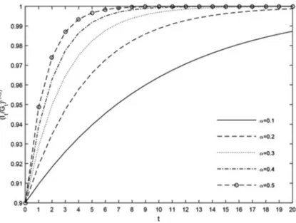
Solving this equation, one finds that the expression for the ratio between revenue and ex­ penditure for any period t starting from initial revenue and expenditure I₀, G₀ is:

(10) It

From this expression it is easy to see that if a e (0,1) then limt→∞ _G =1, from which it t

follows that revenues and expenditures tend to equalize in the long run, and therefore the sys­ tem’s deficit will tend to 0.

Figure 1 shows the evolution of the ratio revenues to expenditures for twenty periods as­ suming that I₀/G₀ = 0.9, for different values of the parameter a. As expected, the smaller the value of a, the longer it takes to reach budget equilibrium.

Another interesting result is observed when computing the financial results generated by the model over the course of years. Let H be the surplus (or deficit) generated by the system_t in the year t. From the equilibrium condition, if in the initial period t=0 the system is in equi­ librium it remains so for any future period. Otherwise, the deficit (or surplus) will be H = I –G_{t t t}, or, which is the same,

H = I (1 + g_I,t) – (Gs _{(1 + g ) + G}a₎

t t–1 t t t

Substituting the revaluation factor (9) in the above expression and simplifying, one has:

Now, considering that one can finally calcu­

late the financial result for any time t from the initial conditions of the system:

There are two very important aspects to note in this result. Firstly, the surplus (or deficit) of the system only depends on the initial state of the system, the increase in revenues, and the

))(1-a)t

choice of the parameter a. Secondly, because of the term (1 – (G₀/I₀ , if the ratio G₀/I₀ is less than unity (and therefore revenues initially exceed expenditures), the value of H will al-_t ways be positive, and the system will incur in surplus indefinitely. On the contrary, if in the initial state expenditures exceed revenues, then the financial result will always be negative, so that the system will incur deficits indefinitely. Therefore, it would be impossible for the Social Security Reserve Fund to accumulate any possible surpluses because there would never be any. Finally, one should observe that the model is set out in a way that does not allow the system to absorb the accumulated debt. The same would be the case with any deficit that might be generated, which would not be reabsorbed and would accumulate in the form of a debt that can not be liquidated. So, the only method that allows the model to avoid a permanent deficit is to impose an upper bound on the revaluations. Then financial surpluses would not impact in their full value on the surviving pensions, being instead capable of covering potential shortfalls.

We propose an alternative method rather than imposing an upper bound to the revaluation based on establishing a budgetary equilibrium that includes the gradual absorption of the debt. Denoting by D the debt in year t, one has for t=1,2, ..._t

Note that a positive value of debt will mean an excess of resources, while a negative value will mean that there are outstanding accumulated deficits. Since we demonstrated above the

convergence of the deficit and its monotonic character with respect to the initial conditions, the debt will also be bounded. Now, if the equilibrium equation is of the form:

lim I + D

and since the results above prove that t+1 t

t→∞ _G =1, as the periods pass the revenues plus t+1

the debt will converge to the expenditures. In this case, the revaluation factor takes the form: (11) For the particular case of a = 1, all the debt is transferred to the existing pensions in a single period, and is therefore settled in that one period.

Example 1 (Continued) Let’s suppose that in our small system exists a debt of

D_t-1 = –1000 in year t–1 and D_t = –4000 in year t. For a value of a=1, all debt is absorbed in t+1 with a revaluation of –7.32%, according to expression (11). For a value of a=0.3, the re­ valuation is smaller, –0.28%, because the debt absorption is shared among several future years.

4.2. The moving averages

The most complex extension of the model, with the aim to smooth out the impact of the economic cycle, is to consider arithmetic and geometric means for the computation of the ele­ ments involved in determining the revaluation index. Law 23/2013 fixes at eleven the number of years to use, centred on t+1, the year for which the revaluation is calculated.

Perhaps the main criticism of the use of means is the need to estimate the expenditures and revenues of the system for the future six years, i.e., from year t+1 to year t+6. According to Law 23/2013, the Ministry of Economy and Finance shall provide the necessary forecasts of macro­ economic variables needed for this estimation. That raises the need to contrast the accurateness of the projections, because from a proper selection of the variables involved the revaluation could be set arbitrarily. This point is crucial, since one of the key advantages of implementing an auto­ matic balancing mechanism is to avoid, insofar as possible, government intervention.

In this subsection, we wish to reflect on other methodologically problematic issues which arise from the introduction of moving averages to compute the revaluation index using Equa­ tion (1). In particular, we shall discuss two major drawbacks. The first is that Equation (1) has no analytical solution. And the second is that the model presents problems of dynamic consis­ tency, so that there is no guarantee that revenues and expenditures will compensate each other in either the short or the long terms.

To demonstrate the problem of the lack of an analytical solution, let us recall that pension expenditure in year t+1 is given by G = Gs _{(1+g ) + G}a _{. If one denotes by G}b _{the ex­}

t+1 t+1 t+1 t+1 t+1

penditure produced by exits from the system, i.e., the expenditure produced by those pensions that do not survive t+1, then one has that G = Gs _{. Thus, substituting, one obtains:}

t+1 + Gb

t t+1

G = (G – Gb _{) (1 + g ) + G}a t+1 t t+1 t+1 t+1

In this way, one year’s expenditure can be related to the expenditure of the previous year. Continuing with the process, one can obtain the expression of expenditure for the period t +n:

s n n−1 a b n a

Gt n + =Gt 1 + Πi=1 (1+ gt i + ) +

∑

++

ion in year t+1 will explicitly affect the expenditure in all future periods.

In Equation (1), the term G*

t+1 =P10 i=0 Gt+1–4 represents the geometric mean of expenditures

centred on t+1. The product of these terms, defined above in (12), will lead to a sum of terms in (1+g_t+1) raised to different powers, the largest of them being the eleventh power. For this reason, since it will be impossible to isolate the factor (1+g ) from the term G* _{, Equation}

t+1 t+1

(1) will have no analytical solution. The revaluation may, however, be computed numerically, as we shall show in the next section.

The second problem to consider with the use of moving averages is the model’s lack of dynamic consistency. In calculating the revaluation index for a given year, one is choosing the index which satisfies the corresponding equilibrium condition. However, there is no criteria that guarantees that once the revaluation for the following period is computed, the previous equilibrium condition is still satisfied. So, a proper revaluation path should be computed to tackle the dynamic inconsistency problem. However, since multiple criteria can be established to compute the revaluation path, we would find a multiplicity of solutions to the problem. The believe that the Law should clearly specify a unique criteria to compute the an optimal revalu­ ation path, thus avoiding both the problem of dynamic inconsistency and multiplicity of solu­ tions to the problem.

The issue of dynamic inconsistency has been studied in Moral-Arce and Geli (2015) and Devesa et al. (2015) with similar methodology. In their papers, the authors suggest to use a procedure based on an iterative method to force the equilibrium condition to be satisfied for every period during a fixed temporal horizon. In this way, if the projections are correct, the computation of the revaluation for one given period takes into account that the equilibrium condition for the subsequent periods must also be satisfied. In Section 5 we will discuss this solution, and we will provide an alternative model for pension revaluation to overcome the dynamic inconsistency problem.

5. The dynamic optimization approach

In this section, we propose an alternative methodology for computing optimal revaluation paths based on dynamic optimization techniques. Our aim is to mimic the characteristics of the revaluation formula in Law 23/2013, that is, the attainment of financial equilibrium through the revaluation of surviving pensions, but with a simpler and more flexible approach. We propose a functional that may provide smoother optimal revaluation paths than the obtained using the revaluation formula (1), and allows for greater flexibility in deciding the economic and social objectives to attain. Moreover, it simplifies the problem excluding the use moving averages.

In order to compare our proposal with previous literature, we first describe the iterative method in Moral-Arce and Geli (2015). The procedure is as follows:

1. Assume an initial trajectory of the expenditures from t+1 to a fixed horizon T, so that in the last period expenditures equal revenues.

2. Numerically compute the revaluation that solves the revaluation formula for every period from t+1 to T.

3. Using the above values for the revaluation, iterate to compute values for the expendi­ tures from period t+1 to period T.

4. Use the new values of expenditures to compute new values of revaluation for every period from t+1 to T.

5. Iterate until convergence. An adequate criteria might be iterate until the difference of value of revaluation between iterations is smaller or equal to 0.01%.

The authors advocate the use of computational software like Excel’s VBA to perform the computations.

From our point of view, a similar but easier description of this idea is not to not compute the revaluation using an iterative procedure but instead solving a system of non-linear equa­ tions so that the equilibrium condition is satisfied simultaneously for periods t+1 to T.

Formally, we aim to obtain the variables g_i, for i = t+1,...T, that solve the system:

(13)

The first set of equations ensure that the revaluation formula is satisfied for periods t+1 to –

as commented in Section 3. The second set of equations describes the dynamic of the total expenditure. Finally, the last equation guarantees the budget equilibrium in the last period. As will be seen in the numerical example of the next section, results are very close to those ob­ tained through the iterative method.

Note that in order to compute the revaluation of final year T, according to the formula (1) projections for years T+1 to T+6 are needed. We propose a small modification in formula (1) in years T to T–4 to avoid these projections. The modification is as follows: in year T, no mov­ ing average is employed; in year T–1 the moving average is computed using three years centred in T–1; in year T–2 the moving average is computed using five years, centred in T–2, and so on. In year T–5 the revaluation formula is employed as usual. Since in the last years expendi­ tures must converge to revenues, the modification in the formula should not be significant and avoids to project the variables for six extra years.

After detailing the iterative procedure, we describe an alternative method to obtain the g_i variables through a dynamic optimization model. This approach provides a wide range of pos­ sibilities, allowing us to consider alternative functionals to choose the optimal revaluation path. For example, Haberman and Zimbidis (2002) and Pantelous and Zimbidis (2008) are examples of works using optimal control methods to compute trajectories of key variables of a Social Security system. Recently, Godínez-Olivares et al. (2015) introduced as a control variable the indexation of pensions jointly with the contribution rates and retirement ages in a dynamic programming setting. However, their framework is not suited to our particular problem, where revaluation only affects to surviving pensions and not to all pensions.

We consider a policy that combines two objectives. Firstly, revaluations should be close to a given reference level c (possibly 0). The level c does not need to be constant, for example, can be set as the projected CPI for future periods. However, if it is set constant, it ensures a small variability between successive revaluations. Secondly, the revaluations must be such that every period expenditures are close to revenues. The importance of each target can be weight­ ed through a parameter u e [0,1]. For simplicity we consider constant weights. However, the weighting of objectives can be a function of time, for example, if we prefer to prioritize in the first periods a small pension revaluation and gradually put more emphasis to the second objec­ tive, ensuring the budget equilibrium in the final periods.

In our model we also consider the possibility of assigning a higher weight to the attainment of the objectives during the first periods relative to the final periods. It is done through of an inter­ temporal correction factor d > 0. A value of d < 0 puts more weight into the first periods, where­ as a value of d > 0 weights more the future. The value of parameter d reflects the inter-temporal cost of delaying the attainment of objectives, possibly including the cost of incurring in deficit.

Thus, our problem is:

subject to:

G = GF _{i i}+(G – . G_i–1 0 5 _i b )(1+ )+0.5Gg _{i i} a , i t= +1, ..., T;1

IT =GT

which can be solved with an appropriate numerical software. In order to compare our results to others from related bibliography, in the next section we will use Excel’s VBA to exemplify the computations3 _.

6. Numerical results

In this section, we shall present a numerical example of the applicability of the revaluation index of Spanish pensions, illustrating results obtained in the foregoing sections. We shall compare the optimal revaluation paths obtained using the three methods described in Section 5: using an iterative procedure, solving the system (13) and solving problem (14).

We take 2014 as the reference year t, and we set the final period T in the year 2030. Thus, we will obtain the revaluation from year t+1 = 2015 to year T = 2030.

The required data is obtained from mixed sources. Expenditure and revenue data for the period from t–5 = 2009 to t = 2014 is taken from Moral-Arce and Geli (2015). Data related to the pension revaluation for the years 2009-2014, it is obtained from the Social Security. Note that, for the 2013 pension revaluation, the law Royal Decree-Law 29/2012 establishes a differ­ ent type of revaluation which depends on the amount of the pension. Although the datum for the exact percentage of the overall revaluation is not available, we estimated it to be from the distribution of pensions by intervals of amount from the Statistical Report of the National So­ cial Security Institute for the year 2012.

Since the purpose of this section is not to calculate with precision the revaluation index for 2015 but to illustrate some of the issues that have been discussed in the preceding sections, we shall make simple assumptions based of past data for the estimates of the variables involved [for an in-depth methodological discussion of the revenue and expenditure forecasts, see AIReF (2014)]. We assume yearly increments of revenue of 3%. The rate of newly entering pensions and exits with respect to the total number of pensions is 6% and 4.50%, respectively. The yearly variation of mean pension for exiting pensions is 2%, and 4% for new entries. Other expenditure, i.e., expenditure not derived from pension amounts, increases at 2%.

Table 1 collects the computation of the revaluation path and related variables applying the iterative procedure. As expected, negative revaluations are obtained in first periods to contain expenditure. Once the expenditure has been contained, the following periods obtain a positive revaluation. In order to obtain a clear comparison of the revaluation paths between methods, in this example we do not consider bounds for the revaluations. Note that in practice, the use of bounds would constrain the set of feasible solutions.

Table 1

REVALUATION RESULTS USING THE ITERATIVE PROCEDURE Year Revalua­_{tion mill euros)} Revenue Pension (mill

euros) Other expendi­ ture (mill euros) Number of pensions Mean Pension Substitu­ tion Effect t-5 2009 2.0% 117,397.00 8,614,876 760.68 t-4 2010 2.3% 116,458.20 95,698.90 17,945.10 8,749,054 781.30 2.44% t-3 2011 0.00% 116,119.00 99,533.95 16,882.10 8,871,435 801.40 2.57% t-2 2012 1.00% 113,081.30 103,504.12 15,526.10 9,008,348 820.70 1.41% t-1 2013 1.55% 112,935.00 108,568.26 14,768.40 9,154,617 847.10 1.72% t 2014 0.25% 117,994.00 112,205.47 15,320.40 9,270,881 864.50 1.71% t+1 2015 -0.51% 121,533.82 113,404.28 15,626.81 9,409,944 860.82 0.08% t+2 2016 -0.90% 125,179.83 114,317.17 15,939.34 9,551,093 854.93 0.21% t+3 2017 -0.51% 128,935.23 115,813.92 16,258.13 9,694,359 853.32 0.32% t+4 2018 0.04% 132,803.29 118,091.76 16,583.29 9,839,775 857.25 0.42% t+5 2019 0.52% 136,787.39 121,108.30 16,914.96 9,987,371 866.15 0.51% t+6 2020 0.61% 140,891.01 124,431.39 17,253.26 10,137,182 876.77 0.62% t+7 2021 0.67% 145,117.74 128,055.48 17,598.32 10,289,240 888.97 0.72% t+8 2022 0.60% 149,471.27 131,828.14 17,950.29 10,443,578 901.64 0.83% t+9 2023 0.61% 153,955.41 135,870.74 18,309.30 10,600,232 915.55 0.93% t+10 2024 0.46% 158,574.07 139,981.50 18,675.48 10,759,235 929.31 1.04% t+11 2025 0.34% 163,331.29 144,217.06 19,048.99 10,920,624 943.28 1.16% t+12 2026 0.62% 168,231.23 149,136.21 19,429.97 11,084,433 961.04 1.26% t+13 2027 0.15% 173,278.17 153,696.74 19,818.57 11,250,700 975.79 1.39% t+14 2028 0.12% 178,476.51 158,530.18 20,214.94 11,419,460 991.60 1.51% t+15 2029 0.04% 183,830.81 163,590.89 20,619.24 11,590,752 1008.14 1.63% t+16 2030 -0.11% 189,345.73 168,775.33 21,031.63 11,764,614 1024.72 1.75%

Source: Authors’ elaboration

Similar path can be obtained solving the system (13). Results are collected in Table 2. As seen, the revaluation path is very similar, with small variations in the last periods due to the use of the terminal condition.

Table 2

REVALUATION RESULTS SOLVING THE SYSTEM OF EQUATIONS

2015 2016 2017 2018 2019 2020 2021 2022

–0.52% –0.82% –0.50% 0.03% 0.48% 0.52% 0.61% 0.61%

2023 2024 2025 2026 2027 2028 2029 2030

0.58% 0.51% 0.43% 0.70% –0.15% 0.11% –0.01% –0.14%

Finally, we compute the optimal revaluation path obtained by solving problem (14). We set the parameters c, u and d to c = 0.25%, u = 0.85 and d = 0.95. A high value of u indicates that we assign more weight to obtain a smaller revaluation that to balance the budget, where a value of d < 1 indicates that we assign more weight to the attainment of the objectives in the first periods than the last periods. Table 3 displays the results of this baseline case. Similar to the previous cases, negative revaluations are obtained in the firsts periods in order to cope with the unbalanced budget, followed by and small positive revaluations in the next periods.

Table 3

REVALUATION RESULTS USING THE DYNAMIC OPTIMIZATION APPROACH Year Revalua­_{tion mill euros)} Revenue Pension (mill

euros) Other expendi­ ture (mill euros) Number of pensions Mean Pension Substitu­ tion Effect t-5 2009 2.0% 117,397.00 8,614,876 760.68 0.00% t-4 2010 2.3% 116,458.20 95,698.90 17,945.10 8,749,054 781.30 2.44% t-3 2011 0.00% 116,119.00 99,533.95 16,882.10 8,871,435 801.40 2.57% t-2 2012 1.00% 113,081.30 103,504.12 15,526.10 9,008,348 820.70 1.41% t-1 2013 1.55% 112,935.00 108,568.26 14,768.40 9,154,617 847.10 1.72% t 2014 0.25% 117,994.00 112,205.47 15,320.40 9,270,881 864.50 1.71% t+1 2015 -1.32% 121,533.82 112,510.74 15,626.81 9,409,944 854.04 0.11% t+2 2016 -0.64% 125,179.83 113,716.73 15,939.34 9,551,093 850.44 0.21% t+3 2017 -0.16% 128,935.23 115,599.37 16,258.13 9,694,359 851.74 0.32% t+4 2018 0.15% 132,803.29 118,003.98 16,583.29 9,839,775 856.61 0.42% t+5 2019 0.35% 136,787.39 120,822.35 16,914.96 9,987,371 864.11 0.52% t+6 2020 0.47% 140,891.01 123,978.31 17,253.26 10,137,182 873.58 0.63% t+7 2021 0.52% 145,117.74 127,418.36 17,598.32 10,289,240 884.55 0.73% t+8 2022 0.53% 149,471.27 131,105.40 17,950.29 10,443,578 896.69 0.84% t+9 2023 0.51% 153,955.41 135,014.62 18,309.30 10,600,232 909.78 0.95% t+10 2024 0.47% 158,574.07 139,130.73 18,675.48 10,759,235 923.66 1.06% t+11 2025 0.41% 163,331.29 143,446.35 19,048.99 10,920,624 938.24 1.17% t+12 2026 0.34% 168,231.23 147,961.37 19,429.97 11,084,433 953.47 1.29% t+13 2027 0.26% 173,278.17 152,683.21 19,818.57 11,250,700 969.36 1.40% t+14 2028 0.19% 178,476.51 157,628.08 20,214.94 11,419,460 985.96 1.52% t+15 2029 0.13% 183,830.81 162,823.77 20,619.24 11,590,752 1003.41 1.64% t+16 2030 0.08% 189,345.73 168,314.11 21,031.63 11,764,614 1021.92 1.76%

Source: Authors’ elaboration

To illustrate the flexibility of the dynamic optimization approach, we also compute the optimal revaluation path for different combinations of parameters u and d, while maintaining the parameter c set to a constant value of c = 0.25%. Table 4 reports the results.

Table 4

OPTIMAL REVALUATION PATHS FOR DIFFERENT PARAMETER VALUES

u = 0.85 u = 0.85 u = 0.85 u = 0.5 u = 0.95 d = 0.95 d = 0.5 d = 1.5 d = 0.95 d = 0.95 -1.32% -0.92% -1.56% -3.60% -0.44% -0.64% -0.55% -0.48% -0.87% -0.22% -0.16% -0.25% 0.09% 0.28% -0.05% 0.15% -0.01% 0.37% 0.74% 0.08% 0.35% 0.17% 0.50% 0.89% 0.18% 0.47% 0.30% 0.53% 0.90% 0.25% 0.52% 0.39% 0.51% 0.85% 0.29% 0.53% 0.44% 0.47% 0.77% 0.31% 0.51% 0.47% 0.41% 0.67% 0.32% 0.47% 0.47% 0.35% 0.57% 0.31% 0.41% 0.44% 0.29% 0.46% 0.30% 0.34% 0.41% 0.24% 0.34% 0.27% 0.26% 0.36% 0.19% 0.23% 0.24% 0.19% 0.30% 0.16% 0.11% 0.21% 0.13% 0.13% 0.14% 0.01% 0.19% 0.08% 0.12% 0.15% -0.08% 0.17%

Source: Authors’ elaboration

The first column contains the results of the baseline case, the same as in Table 3 (u = 0.85, d = 0.95). The second column reflects the combination u = 0.85, d = 0.5. Compared to the baseline case, because of the smaller value of d, it puts more weight to the objective of obtain­ ing a small revaluation during the first periods. Therefore, the optimal revaluations are smaller in absolute value for the first periods but larger for the final periods. In opposition, the combi­ nation u = 0.85, d = 1.5, in column three, assigns more weight in obtaining smaller revaluations in the last periods, so the adjusting during the first periods is more severe than in the baseline case.

If we modify instead the parameter u, we can smooth out the optimal revaluation path by giving priority to obtain smaller revaluations (setting u to a large value) or we can prioritize to attain the budget equilibrium faster (setting u to a small value). For example, the combination u = 0.5, d = 0.95 yields larger revaluations (in absolute value) in the first periods, since more weight is placed in balancing the budget with respect to the baseline case. The combination u = 0.95, d = 0.95, however, produces a very smooth path, but at the expense of a slower re­ covery of the budget equilibrium.

7. Conclusions

In this paper, we have scrutinized the technical aspects of the computation of the revalua­ tion index of Spain’s pensions. Based on a simplified model, we analysed step by step the ele­ ments that comprise it, starting with the correct definition of the factors involved in its calcula­ tion. We then examined the implications of adding directly the coefficient a to the final expression in order to regulate the rate at which the deficit is reduced, and of the use of moving averages to calculate the magnitudes involved. Several recommendations to improve the legis­ lation have been provided. In particular, the incoherent definition of the expenditures should be addressed. Finally, we established a general dynamic optimization approach to compute the optimal revaluation path in order to cope with the problem of dynamic inconsistency, while exemplifying its use with some numerical results.

Notes

1. Population aged 65 and over as percentage on the population aged 15-64.

2. This definition of revenue and expenditure differs from the Draft’s proposal, which only included the items of current operations (chapters 1 to 4 in expenditure and 1 to 5 in revenue). Thus, items would be excluded that relate to outlays for real property investments and capital transfers, and to revenues from the disposal of real property investments and capital transfers.

3. The Excel file can be downloaded for unrestricted use from the website http://www.ub.edu/grpen sions/difusion/

­

References

AIReF (2014), “Opinión sobre la determinación del Índice Revalorización de las Pensiones 2015”, Mimeo.

Börsch-Supan, A. (2012), “Entitlement reforms in Europe: Policy mixes in the current pension reform process”, NBER Working Paper Series No. 18009.

Börsch-Supan, A., Reil-Held, A. and Wilke, C.  B. (2003), “How to make a defined benefit system sustainable: The “sustainability factor” in the German Benefit Indexation Formula”, MEA Discus­ sion Paper 037-03.

Canada Pension Plan (2007), “Optimal funding of the Canada pension plan. Office of the Chief Actu­ ary”, Actuarial Study No. 6.

Conde-Ruiz, J. and Alonso, J. (2004), “El futuro de las pensiones en España: Perspectivas y lecciones”, Información Comercial Española (ICE), 85: 155-174.

De las Heras, A., Gosálbez, M. B. and Hernández, D. (2014), “The sustainability factor and the Span­ ish public pension system”, Economía Española y Protección Social, VI: 119-157.

Devesa, J., Devesa, M., Meneu, R., Domínguez, I. and Encinas, B. (2015), “El Índice de Revalorización de las Pensiones (IRP) y su impacto sobre el sistema de pensiones español”, Revista de Economía Aplicada, 1-23.

Diamond, P. A. (2004), “Social Security”, The American Economic Review, 94(1): 1-24.

Díaz-Giménez, J. and Díaz-Saavedra, J. (2009), “Delaying retirement in Spain”, Review of Economic Dynamics, 12: 147-167.

European Commission (2015), The 2015 Ageing Report: Economic budgetary projections for the 28 UE member states (2013-2060).

Godínez-Olivares, H., Boado-Penas, M. del C. and Pantelous, A. (2015), “How to finance pensions: Optimal strategies for pay-as-you-go pension systems”, Journal of Forecasting, 35: 13-33. Haberman, S. and Zimbidis, A. (2002), “An investigation of the pay-as-you-go financing method using

a contingency fund and optimal control techniques”, North American Actuarial Journal, 6: 60-75. Jimeno, J., Rojas, J. and Puente, S. (2008), “Modelling the impact of aging in social security expendi­

tures”, Economic Modelling, 25: 147-167.

Moral-Arce, I. and Geli, F. (2015), “El índice de revalorización de las pensiones (IRP): Propuestas de solución del problema de la circularidad”, Documento de Trabajo DT/2015/1, AIReF.

Pantelous, A. and Zimbidis, A. (2008), “Dynamic reforming of a quasi pay-as-you-go social security system within a discrete stochastic multidimensional framework using optimal control methods”, Applicationes Mathematicae, 35: 121-144.

Sakamoto, J. (2005), “Japan’s pension reform. Social Protection”, Discussion Paper No. 0541, Wash­ ington, DC: World Bank.

Sakamoto, J. (2008), “Roles of the social security pension schemes and the minimum benefit level under the automatic balancing mechasim”, Nomura Research Papers No. 125.

Sánchez-Martín, A.  R. (2010), “Endogenous retirement and public system reform in Spain”, Eco­ nomic Modelling, 27: 336-349.

Sánchez-Martín, A. R. (2014), “The automatic adjustment of pension expenditures in Spain: An evalu­ ation of the 2013 pension reform”, Documento de Trabajo n. 1420, Banco de España.

Settergren, O. (2001), “The automatic balance mechanism of the Swedish pension system-a non­ technical introduction”, Wirtschaftspolitische Blätter, 4: 339-349.

Turner, J. A. (2009), Social security financing: Automatic adjustments to restore solvency, Washington, DC: AARP Public Policy Institute.

Vidal-Meliá, C., Boado-Penas, M. and Settergren, O. (2009), “Automatic balance mechanisms in pay­ as-you-go pension systems”, The Geneva Papers on Risk and Insurance-Issues and Practice, 34: 287-317.

Resumen

Este artículo revisa los aspectos metodológicos del índice de revalorización de las pensiones españolas desarrollado a través de la Ley 23/2013 reguladora del Factor de Sostenibilidad y del Índice de Re­ valorización del Sistema de Pensiones de la Seguridad Social. A partir del desglose de los elementos que conforman el índice de revalorización, se exponen los problemas formales y de interpretación que presenta. Finalmente, un modelo alternativo basado en técnicas de optimización dinámica es pro­ puesto y su uso ilustrado con ejemplos numéricos.

Palabras clave: índice de revalorización, mecanismos de ajuste automáticos, Seguridad Social. Clasificación JEL: H55, J26