A Numerical Technique for Determining the Internal Field in Biological Bodies Exposed to Electromagnetic Fields

(1)

UNIVERSITY

OF TRENTO

DIPARTIMENTO DI INGEGNERIA E SCIENZA DELL’INFORMAZIONE 38123 Povo – Trento (Italy), Via Sommarive 14

http://www.disi.unitn.it

A NUMERICAL TECHNIQUE FOR DETERMINING THE INTERNAL FIELD IN BIOLOGICAL BODIES EXPOSED TO ELECTROMAGNETIC FIELDS

S. Caorsi, E. Bermani, A. Massa, M. Pastorino, A. Rosani, and A. Randazzo

January 2004

(2)

(3)

A numerical technique for determining the internal field in biological bodies

exposed to electromagnetic fields

by S. Caorsi (1)(2), E. Bermani (1)(3), A. Massa (1)(3), M. Pastorino (1)(4), A. Rosani (3), and A. Randazzo (4)

(1) ICEmB - Interuniversity Center for the Interaction Between Electromagnetic Fiels and Biosystems.

(2) Department of Electronics University of Pavia

Via Ferrata 1

27100 Pavia, ITALY.

Phone: + 39 0382505661 Fax: +39 0382422583 e-mail: caorsi@ele.unipv.it (3) Department of Information and Communication Technology

University of Trento Via Sommarive 14 I-38050 Trento, ITALY.

Phone: +39 0461882057 Fax: +39 0461881696 e-mail: andrea.massa@ing.unitn.it (4) Department of Biophysical and Electronic Engineering

University of Genoa Via Opera Pia 11A 16145, Genova, ITALY.

(4)

Abstract

In this paper, the field prediction inside biological bodies exposed to electromagnetic incident waves is addressed by considering inverse scattering techniques. In particular, the aim is to evaluate the possibility of limiting the test area in order to strongly reduce the computational time, ensuring, at the same time, a quite accurate solution. The approach is based on separating the scattering contributions of the region under test and the other part of the biological body. The starting point is represented by the inverse-scattering equations, which are recast as a functional to be minimized. A Green's function approach is then developed in order to include an approximate knowledge (a model) of the biological body. The possible application of the approach for diagnostic purposes is also discussed.

1. Introduction.

In the last years, there has been a growing interest in numerical methods for determining the internal field and related quantities (e.g., the specific absorption rate (SAR)) of biological bodies exposed to electromagnetic radiation, especially due to mobile phones. Potentialities and limitations of several classical methods have been discussed in a wide number of papers (see, for example, papers [1]-[4] and the references therein). Among them, one can mention, with an "historical" sorting, the method of moments (MM) [5], the finite element method (FEM) [6], the finite difference time domain (FDTD) method [3] and a large number of recently proposed hybrid methods, which are aimed to reduce some limiting factor of the previous classical methods and, sometimes, to combine the advantages of two or more basic formulations (e.g., FEM, MM-FDTD) in order to deal with different parts of the body under test [2].

The above-mentioned methods are applied to solve the integral/differential equations of the electromagnetic scattering problem, which represent the mathematical starting point of the approaches for field prediction in biological applications.

These methods, which have been used with great success in several applications, are based on a forward scattering formulation, in which the geometric and dielectric characteristics of the body under test are assumed to represent completely known information. However, it has been shown in several works that small uncertainties in the geometric/dielectric properties of the body may result in significant differences in the field distributions. From this point of view, it is not surprising that

(5)

results different from the expected ones have been obtained anytime that more sophisticated models of the source and of the biological body have been introduced.

The possibility of considering a specific biological body, quite independently from a complete knowledge of the geometric and dielectric properties of its structures has suggested the study of inverse approaches for the field prediction [7]. These approaches are based on the inverse scattering problem, as opposed to the classical methods, which are based, as previously mentioned, on the forward scattering approach.

To apply an inverse scattering method, one needs to know the scattered electric field at certain locations outside the biological body under test. However, although the measurement of field values does not represent anymore a technical problem, it should be realized that this requirement constitutes a limiting factor of the approach. The major limitation of the approach is however represented by the computational difficulties inherent any numerical inverse problem. Such difficulties are related to the ill-posed nature of the problems [8]. We will discuss this point later on. Nevertheless, the great potential advantage of the approach is related to the possibility of predicting the internal field, in principle, without any knowledge of the internal structure of the biological body. Obviously, if some information on the body is available, it can be inserted as a priori knowledge, usually allowing a speed up of the computation and a significant reduction of the ill-conditioning of the problem.

Moreover, the inverse approach is also of interest for diagnostic purposes. In fact, in this case, the internal field is not of interest, but the geometric and dielectric properties of internal organs have to be retrieved. The key point is that both the field and the geometric/dielectric properties are unknown in the inverse scattering approach (except in the case in which some a priori information is available, e.g., a CT image of the body defining boundaries between different biological tissues). As previously mentioned, the inverse scattering problem is usually strongly ill-posed. The numerical counterpart of the problem is ill-conditioned. Consequently, small errors in the measurement data result in large errors in the field prediction. To this end, the inverse problem is commonly recast as a global optimization problem, in which a suitable functional is defined and minimized [9]. The functional can take into account both the "data equation" (which relates the measured samples of the external field to the internal field and the dielectric properties) and the "state equation" (which imposes that the internal field and the dielectric properties be consistent with the unperturbed exposure field). The state equation can be also considered as a regularization term in the functional to be minimized. Other regularization terms can be added in order to reduce the search space of the minimization procedure. These terms can include the a priori information on the model. In practical applications, they are usually very important.

(6)

Finally, the functional is minimized by using a deterministic method (e.g., the conjugate gradient method) or a stochastic approach (e.g., the genetic algorithm). In the present paper, following an approach previously developed by the same authors, a hybrid genetic algorithm is applied [10]. In the hybrid genetic algorithm, the classic stochastic scheme of the genetic algorithm is combined with a deterministic method in order to speed up the convergence of the iterative process. It is well known that stochastic methods are usually computationally much more heavy than deterministic approaches, although they are in principle able to find the global solution, relatively independently on the starting point.

2. Mathematical Formulation

Let us consider the cross section of a biological body, which is indicated by A. The distributions of the following dielectric parameters characterize the biological body:

r

ε : Relative dielectric permittivity; σ: Electric conductivity [S/m].

Both distributions are inhomogeneous and these quantities depends on the transversal coordinates x and y. Nonmagnetic tissues are assumed (μ=μ₀).

The biological bodies in exposed to an incident field (assumed here to be transverse-magnetic polarized). It should be noted that, in diagnostic applications, this field is produced by suitable applicators.

A complete discretization of the body is at present impossible for computational reasons. Moreover, in several applications (e.g., in the case of exposure from mobile phones), the accurate distribution of the field is only really needed in limited regions of the biological body. The same holds for diagnostic purposes, where the region to be inspected is usually limited to an organ or a limited part of the body [11][12]. There are several possible approaches to take into account the above consideration. The simplest one is to neglect some regions of the body cross section. The other more sophisticated approach is to use the proper Green's function [13] (in discretized form) for the model. In practice, a model of the cross section is assumed to be known, and the "scattering" is attributed to a limited region of the body, which is investigated by considering as unknown the internal field and/or the dielectric parameters (more precisely, the variations of these parameters with respect to the assumed model).

(7)

The cross section A is partitioned into partitions not overlapping. It results , where denotes the area of the n-th partition of A, whose center is indicated by . The interest area includes N (≤P) subdomains indexed by n = 1,..., N.

P = ∑ = P n n A A 1 n A

(

_n _n n = x ,y x

)

Each subdomain is characterized by the complex dielectric permittivity

0 ωε σ − ε = ε n r r j ~ n n (1)

As previously mentioned, the scattered electric field is measured at M locations inside a proper observation domain O not overlapping with A. The measured values of the scattered electric field are denoted by (transverse-magnetic conditions are assumed; consequently, the above quantity refers to the axial component of the field vector). The M values are related to the internal field to be predicted by the following integral equation [14]

s m E s m E

[

~

]

E G

(

x,x

)

dx E P n A m t n r s m n n ∑ ε − ∫∫ = =1 1 0 (2)

where E_nt denotes the total internal field in the n-th subdomain of A,G₀

(

x,x_m

)

is Green's function for free space, and x_m indicates the location of the m-th measurement point.

As mentioned in the Introduction, the simplest approach to deal with a reduced test area is to choose it in order that the effect of the presence of the P-N subdomains N+1,N+2,...,P be negligible. This approach is possible, although with a certain degree of approximation, in imaging applications, where the incident field is fixed by the operator, or in the field prediction inside exposed bodies when the illumination conditions allows a priori to infer that limited regions of high field are present (e.g., in the case of mobile phones). A numerical assessment concerning this approach is reported in Section 3. In this case, the summation in equation (2) is "limited" to index N. Equation (2) results in an inverse scattering problem, which is linear, if

n

r

~_{ε is known, otherwise it is} nonlinear. This inverse problem can be solved by using one of the recently developed iterative approaches (see, for example, [15] and the references therein).

(8)

0 n n n r r r ~ ~ ~_ε ₌_Δ_ε ₊_ε _{n = 1,...,N (3)}

where denotes the relative dielectric permittivity of a model of cross section. The other part of the scatterer is assumed to be exactly characterized by the known model. For the "object" constituted by 0 n r ~_ε n r ~_ε

Δ , n = 1,...,N, the "propagation medium" is an inhomogeneous medium characterized by 0

n

r

~_{ε for n = 1,...,P.}

In this case, the inverse scattering problem is governed by the following equation

[

~

]

E G

(

x,x

)

dx E N n A m N t n r s m n n ∑ Δε − ∫∫ = =1 1 (4)

where the inhomogeneous Green's function G_N

(

x,x_m

)

can be obtained by solving off line and once for all the following integral equation

(

)

[ ]

(

)

[

]

(

)

(

n P N n A m N r N n A m N r n N , ~ G , d ~ G , d G , G n n n n x x x xx x x x x x ₀ 1 1 0 1 1 − ∑ ε − ∫∫ = ∑ ε − ∫∫ − + = =

)

(5)

Solving equation (5) corresponds to solve a classic forward scattering problem. When the values of the inhomogeneous Green's function have been calculated by solving (5), the inverse scattering problem can be re-formulated by using (4), exactly as previously described.

As discussed in the Introduction, due to the ill-conditioning of the inverse problem, the "state equation" is usually associated to the "data equation" (equation (2), with P replaced by N, or equation (4)). The state equation imposes that the internal field and the dielectric properties be consistent with the unperturbed exposure field, and it is given by

(6)

[

]

( )

i q N n t n qn A q r G , d E E ~ n n =− ∑ ⎭ ⎬ ⎫ ⎩ ⎨ ⎧ δ − ∫∫ − ε =1 1 0 x x x or

[

]

( )

model q N n t n qn A q N r G , d E E ~ n n =− ∑ ⎭ ⎬ ⎫ ⎩ ⎨ ⎧ δ − ∫∫ − ε Δ =1 1 x x x (7)

(9)

where denotes the total internal field in the n-th subdomain; indicates the incident field at the center of the q-th subdomain; is the total field in the same subdomain of the known model (which constitutes the incident field for the "excess of permittivity"); finally, , if n = q,

, otherwise. t n E E_qi el mod q E 1 = δ_qn 0 = δ_qn

Once again, equations (6) and (7) are linear or nonlinear under the same conditions of equations (2) and (4).

The simultaneous solution of the "data" and "state" equations is obtained by defining a suitable functional [9]. In this way, the inverse scattering problem is recasts as an optimization problem. The functional has the following form

data state R

R

J =α +β (8)

where and denotes the square norms of the residuals of the "data equation" ((2), with P replaced by N, or (4)) and the "state equation" ((6) or (7)).

data

R R_state

The minimization of J is performed by using an hybrid genetic algorithm, in which the classic stochastic approach is combined with a conjugate gradient method in order to speed up the convergence of the iterative process. This minimization method has been described in details in [10].

3. Numerical results

Let us consider the geometrical configuration shown in Figure 1, where the cross section of a human head model is surrounded by several measurement points (located on a circumference of radius r = 0.14 m, at angular positions given by ϑ = - 3/4π-i(3π/2M-2), i = 1,...,M (observation _i domain O)). The head model is the same used in [7]. For simplicity, the head cross section is included in square domain, DI, which is partitioned into P subdomains (in practice, since the "air" subdomains are treated as the other subdomains, DI is "equivalent" to region A). A reduce area R is defined, which corresponds to the first N subdomains (test area). The numerical data for the first assessment are the following: P = 32 × 32, M = 32, the incident wave is: 1) a uniform plane wave (simulating far-field illumination conditions); 2) a cylindrical wave produced by a line currents (simulating near-field illumination conditions in the transversal plane).

(10)

Fig. 1 Problem configuration. Head model, test area, and measurement points

The test area is obtained by considering only n rows and m columns of the partitioned domain, corresponding to the test region nearest to the source. The dimension of R is defined as a function of n and m. In particular, it is denoted by R = R(n,m). Consequently, the number of subdomains of a certain test area R(n,m) is given by N = mn, and R(32,32) ≡ DI.

The following errors parameters are defined in order to evaluate the approximation

∑ ∑ − = Ω = = n i m j t DI t ) m , n ( R t DI ij ij ij E E E N 1 1 2 2 1 (9) ∑ ∑ − = Θ = = n i m j t DI t ) m , n ( R t DI ij ij ij E E E N 1 1 2 2 1 (10)

where denotes the total electric field predicted in the partition corresponding to the i-th row and the j-th column, considering the whole cross section DI, and is the same field value in the case in which only the test are R(n,m) is considered.

t DI_ij E t ) m , n ( R ij E

(11)

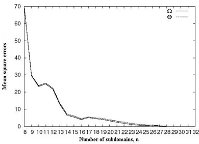
Fig. 2. Errors parameters related to the field prediction,Θ and Ω (equations (9) and (10)) for different values of R(n,n). Plane-wave (far-field) illumination conditions.

Figure 2 gives the errors on the field prediction (plane wave illumination) for various dimensions of R, in the case in which m=n. This figure provides indications concerning the possibility of reducing the test area for a given expected accuracy in the field prediction. Analogous considerations can be drawn from Figure 3, which refers the near-field illumination conditions. The global information represented by parameters Θ and can be verified by considering Figure 4, in which the computed scattered electric field is plotted along (a) the x axis and (b) the y axis for various reduced domains R.

Ω

Fig. 3. Errors parameters related to the field prediction,Θ and Ω (equations (9) and (10)) for different values of R(n,n). Cylindrical-wave (near-field) illumination conditions.

(12)

Fig. 4. Amplitude of the scattered electric field computed along the x and y axes for different reduced test areas. Comparison with the results obtained for the complete cross section.

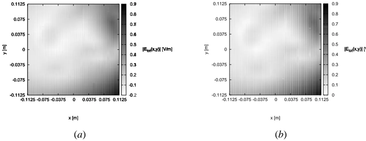
Concerning the approach based on the inhomogeneous Green's function, it has been applied with reference to the model of a human thorax described in [12]. In this case, the frequency is f = 433 MHz and a uniform plane wave illumination is considered. To make more realistic the simulation, the scattered data (at the measurement points) have been affected by a Gaussian noise with zero mean values and corresponding to a signal-to-noise ratio of 30 dBs. A "change" in the dielectric configuration has been assumed. In particular, a square region inside the muscle tissue, corresponding to 25 discretization subdomains, has been considered. For this reduced region R(5,5), we assumed Δ =

n

r

ε~ _{-1.8 + j2.91 , n = 1,...,N (=25). Starting by the unperturbed configuration, the} inhomogeneous Green's function has been calculated by using equation (5). The inverse problem has been solved as described in Section 2 and the results are provided in Figure 5. In particular, the figure shows the (a) original and (b) predicted total electric field (after 100 iterations of the inverse procedure). As can be seen, a very good agreement has been obtained.

(13)

(a) Original distribution. (b) Predicted distribution. 4. Conclusions

In this paper, the use of an inverse approach for the field prediction inside biological bodies has been discussed. The need for reducing the test area leads to consider specific approaches based on models of the biological body under test. For the case in which only an internal region can be considered important for the prediction or in medical imaging applications, a simple domain truncation can be applied. On the contrary, when more accurate (linear or nonlinear) predictions are required, the approach based on the off-line computation of an inhomogeneous Green's function can be applied. In this case, the test region is considered as the "object" to be inspected, which is located into an inhomogeneous propagation medium constituted by an assumed known model of the whole cross section. Due to the strong ill-conditioning of the inverse problem, the results presented in this paper are still preliminary. However, in the authors' opinion, the potential advantages of the approach are very significant, allowing the approach to be further explored.

5. References

1. Bernardi, P., Cavagnaro, M., Pisa, S., and Piuzzi, E., 2001, IEEE Trans. Microwave Theory Tech., 49, 2539.

2. Mangoud, M. A., Abd-Alhameed, R. A., and Excell, P. S., 2000, IEEE Trans. Microwave Theory Tech., 48, 2014.

3. Lazzi, G., and Gandhi, O. P., 2000, IEEE Trans. Antennas Propagat., 48, 1830.

4. Lazzi, G., Gandhi, O. P., and Sullivan, D. S., 2000, IEEE Trans. Microwave Theory Tech., 48, 2033.

5. Hagmann, M. J., and Levine, R. L., 1990, IEEE Trans. Antennas Propagat., 38, 99. 6. Strohbehn, J. W., and Roemer, R. B., 1984, IEEE Trans. Biomedical Eng., 31, 136. 7. Caorsi, S., and Massa, A., 2000, Bioelectromagnetics, 21, 422.

8. Bertero, M., and Boccacci, P., 1998, Introduction to Inverse Problems in Imaging, IOP, Bristol, UK.

9. Pastorino, M., 1998, IEEE Trans. Instrum. Meas., 47, 1419.

10. Caorsi, S., Massa, A., Pastorino, M., and Randazzo, A., 2001, Proc. 31-st European Microwave Conference (EuMC2001), London, 341.

(14)

12. Caorsi, S., Massa, A., and Pastorino, M., 2000, IEEE Trans. Microwave Theory Tech., 48, 1815.

13. Tai C. T., 1971, Dyadic Green's Functions in Electromagnetic Theory, International Textbook Company, New York.

14. Balanis, C. A., 1989, Advanced Enginnering Electromagnetics, John Wiley and Sons, New York.

15. Liu, Q. H., and Zhang, Z. Q., in: Microwave Nondestructive Evaluation and Imaging, 2002, Research Signpost, Trivandrum.