Responses of model plants to metals and non-metals : two case studies

(1)

Università Degli Studi Del Piemonte Orientale

Amedeo Avogadro

Dipartimento di Scienze e Innovazione Tecnologica

PhD course in

Scienze Ambientali – Acque Interne E Agroecosistemi

XXVII Ciclo

Responses Of Model Plants To

Metals And Non-Metals: Two Case Studies.

Nadide AKAY

PhD Supervisor: Prof. Graziella BERTA

PhD Co-Supervisor: Dr. Guido LINGUA

(2)

Amedeo Avogadro University of Eastern Piedmont

Science And Innovation Department

Responses Of Model Plants To Metals And Non-metals: Two Case Studies.

by

Nadide AKAY

A THESIS SUBMITTED IN PARTIAL FULFILLMENT OF THE

REQUIREMENTS FOR THE DEGREE

Doctor Of Philosophy

Approved Thesis Committee:

Prof. Stefano BIFFO

(Università degli Studi di Milano)

Prof. Giovanni LEUZZI

Università degli Studio di Roma “La Sapienza”

Prof. Consolata SINISCALCO Università degli Studi di Torino

(3)

ACKNOWLEDGEMENTS

I would like to extend my sincere thanks and gratitude to:

 my supervisor Prof. Graziella Berta for her patience, guidance, constructive criticism and words of encouragement and to my co-supervisor Dr. Guido. Lingua for his criticizes and his patience throughout the course of this project,

 Dr. Giuseppe Digilio for his assistance, guidance and encouragement throughout the course of this project,

 the Department of Chemistry, Università degli Studi del Piemonte Orientale for their technical assistance, especially to, Prof. Domenico Osella, Dr. Valentina Gianotti, Dr. Lorenzo Tei, Dr. Marco Clericuzio, Dr. Claudio Cassino and Davide Musso.

 my family, for all their support and encouragement,

 my chemistry class students to date from 2010 for filling me with energy,

 all my thesis students for encouragement,

(4)

i

TABLE OF CONTENTS ...i

LIST OF TABLES ...vi

LIST OF FIGURES ...vii

(5)

ii

LIST OF FIGURES

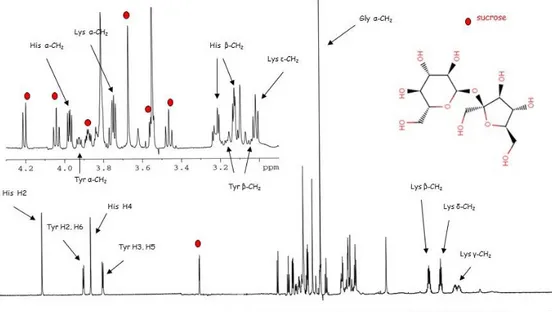
Fig. 1: 1H NMR spectrum of a mixture with assignment of the resonance of several metabolites. Red dots indicate the characteristic sucrose resonances

Fig. 2: 1H NMR spectrum (600 MHz) of blood serum with assignment of the resonance of several metabolites, including lipoproteins. Taken from Beckonert, 2007)

Fig. 3: COSY spectroscopy of benzoic acid.

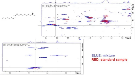
Fig. 4: HSQC spectrum of poplar leaf methanol extract compared to standard sample.

Fig. 5: Superpostion of 14 spectra of P.alba leaf extract, with expansion of selected spectral regions.

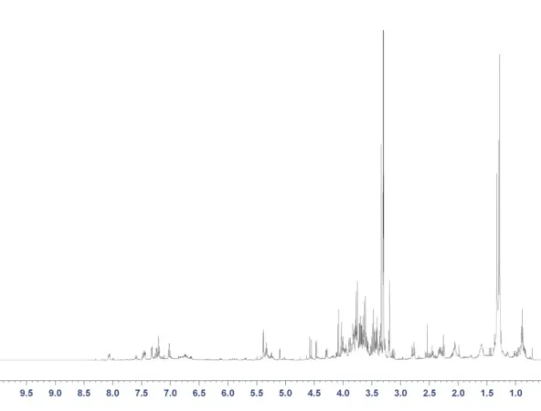
Fig. 6A: Overview of the 1H-NMR spectrum of the methanol extract of leaves from Populus alba (sample CF7, 1D-noesy pulse sequence, with pre-irradiation of the residual MeOH proton, 300 K).

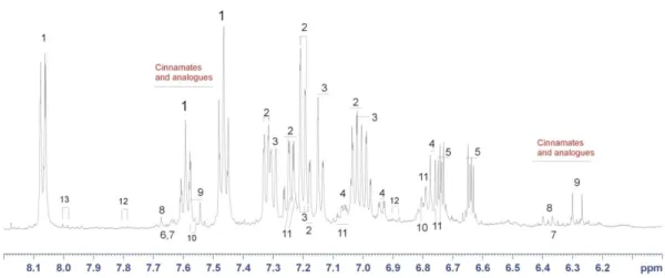
Fig. 6B: Expansion in the range 8.2-6.0 ppm of the 1H-NMR spectrum shown in Fig. 6A (Y-magnification 4x) with resonance assignment

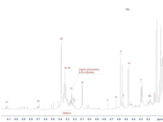
Fig. 6C: Expansion in the range 6.2-4.0 ppm of the 1H-NMR spectrum shown in Fig. 6A (Y-magnification 4x) with resonance assignment

Fig. 6D: Expansion in the range 4.2-2.0 ppm of the 1H-NMR spectrum shown in Fig. 6A (Y-magnification 4x) with resonance assignment

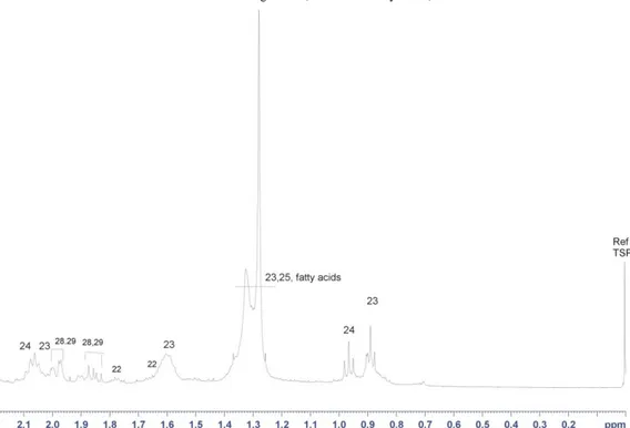
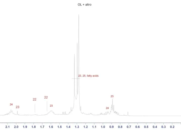
Fig. 6E: Expansion in the range 2.2-0.0 ppm of the 1H-NMR spectrum shown in Fig. 6A (Y-magnification 4x) with resonance assignment

Fig. 7: 1H, 13C HSQC spectrum of Populus alba leaves methanol extract (sample CF7, T=300 K) with assignment

(11)

viii

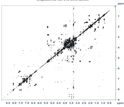
Fig. 7A: Overview of the 1H,1H COSY NMR spectrum of Populus alba leaves methanol extract (sample CF7, T=300 K)

Fig. 7B: Expansion (8.5-4.0 ppm) of the 1H,1H COSY NMR spectrum of

Populus alba leaves methanol extract (sample CF7, T=300 K) with assignment.

Fig. 7C: Expansion (5.6-0.6 ppm) of the 1H,1H COSY NMR spectrum of

Fig. 7D: Expansion (7.9-6.2 ppm) of the 1H,1H COSY NMR spectrum of

Fig. 8A: Overview of the 1H-NMR spectrum of the methanol extract of roots from Populus alba (sample CR7, 1D-NOESY pulse sequence, with pre-irradiation of the residual MeOH proton, 300.0 K).

Fig. 8B: Expansion in the range 8.2-6.0 ppm of the 1H-NMR spectrum shown in Fig. 8A (Y-magnification 4x) with resonance assignment (see Tab. 2 for symbols).

Fig. 8C: Expansion in the range 6.2-4.0 ppm of the 1H-NMR spectrum shown in Fig. 8A (Y magnification 4x) with resonance assignment

Fig. 8D: Expansion in the range 4.2-2.0 ppm of the 1H-NMR spectrum shown in Fig. 8A (Y-magnification 4x) with resonance assignment

Fig. 8E: Expansion in the range 2.2-0.0 ppm of the 1H-NMR spectrum shown in Fig. 8A (Y-magnification 4x) with resonance assignment

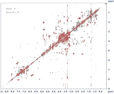
Fig. 9: 1H,13C HSQC spectrum of Populus alba roots methanol extract (sample CR7, T=300 K), (F: Leaf, R: Root).

Fig. 10A: Overview of the 1H,1H COSY NMR spectrum of Populus alba roots methanol extract (sample CR7, T=300 K), (F: Leaf, R: Root).

Fig. 10B: Expansion (8.5-4.5 ppm) of the 1H,1H COSY NMR spectrum of

(12)

ix

Fig. 10C: Expansion (5.0-0.6 ppm) of the 1H,1H COSY NMR spectrum of

Populus alba roots methanol extract (sample CF7, T=300 K), (F: Leaf, R: Root).

Fig. 10D: Expansion (8.2-5.0) ppm) of the 1H,1H COSY NMR spectrum of

Populus alba roots methanol extract (sample CF7, T=300 K), (F: Leaf, R: Root).

Fig. 11: LC-ESI+ mass spectrum (direct infusion) of leaf methanol extract from P. alba with partial assignment of m/z.

Fig. 12: LC-ESI+ mass spectrum (direct infusion) of root methanol extract from P. alba with partial assignment of m/z peaks.

Fig. 13: MS analysis application source code (1).

Fig. 14 : MS analysis application source code (2).

Fig. 17: “leaf 1” - PCA of the 1H-NMR spectra of methanol extracts of leaves from P. alba.

Fig. 18: “leaf 1” - PCA (aromatic region only) of the 1H-NMR spectra of methanol extracts of leaves from P. alba.

Fig. 19: “root 1” - PCA of the 1H-NMR spectra of methanol extracts of roots from P. alba.

Fig. 20: “root 2” PCA of the 1H-NMR spectra of methanol extracts of roots from P. alba.

Fig. 21: Fresh root weight (in grams) of rice plant at the repot.

Fig. 22 : Fresh shoot weight (in grams) of rice plants at repot.

Fig. 23: Dry root weight (in grams) of rice plants at repot.

(13)

x

Fig. 25: P uptake of shoot samples subjected to different treatments.

Fig. 26: As uptake of shoot samples subjected to different treatments.

Fig. 27: N uptake of shoot samples subjected to different treatments.

Fig. 28: C uptake of shoot samples subjected to different treatments.

Fig. 29: H uptake of shoot samples subjected to different treatments.

Fig. 30: S uptake of shoot samples subjected to different treatments.

Fig. 31: P uptake of root samples subjected to different treatments.

Fig. 32: As uptake of root samples subjected to different treatments.

Fig. 33: N uptake of root t samples subjected to different treatments.

Fig. 34: C uptake of root t samples subjected to different treatments.

Fig. 35: H uptake of root t samples subjected to different treatments.

Fig. 36: S uptake of root samples subjected to different treatments.

Fig. 37: Principal Components Scree Plot.

Fig. 38: PC1 vs PC2 loading plot.

Fig. 39: PC1 vs PC3 loading plot.

Fig. 40: PC1 vs PC2 score plot.

Fig. 41: PC1 vs PC2 score plot with labelled data.

Fig. 42: PC1 vs PC2 score plot (labelled).

Fig. 43: Principal Components scree plot (2).

Fig. 44: PC1 vs PC2 loading plot (2).

(14)

xi

Fig. 46: Another scree plot on cleaned data.

Fig. 47: PC1 vs PC2 new loading plot.

Fig. 48: In black shoot samples, in red roots.

Fig. 49: PC1 vs PC2 score plot (labelled-2).

Fig. 50: PC1 vs PC3 loading plot for the cleaned dataset.

Fig. 51: PC1 vs PC3 score plot.

Fig. 52a: PC1 vs PC3 score plot at a different scale (1).

Fig. 52b: PC1 vs PC3 score plot at a different scale (2).

Fig. 53: Coupled data scree plot.

Fig. 54: Coupled data PC1 vs PC2 loading plot.

Fig. 55: Marked PC1 vs PC2 scree plot.

Fig. 56: Scree plot of the final dataset.

(15)

xii

NOMENCLATURE AND ABBREVIATIONS

TNT Trinitrotoluene

TCE Trichloroethylene.

MeOD Deuterated Methanol

ICP-AES Inductively Coupled Plasma Atomic Emission Spectrometer

ICP-MS Inductively Coupled Plasma Mass Spectrometer

NMR Nuclear Magnetic Resonance

HSQC Heteronuclear Single Quantum Coherence

NOESY Nuclear Overhauser Effect Spectroscopy

COSY Correlation Spectroscopy

TSP 3-(trimethylsilyl)-2,2,3,3-tetradeuteropropionate

TFA Trifluoroacetic

amu Atomic Mass Units

ESI-MS Electrospray Ionization Mass Spectrum

HYV High Yielding Variety

DW Dry Weight

FW Fresh Weight

nd Not Detected

FAO Food And Agriculture Organization Of The United Nations

WHO World Health Organization

(16)

1

Chapter 1: Soil Pollution

1.1 Introduction To Soil Pollution

Soil pollution is the phenomenon of the alteration of the chemical composition of the soil caused by human activity (Erfan-Manesh and Afiuni 2005). This kind of alteration of chemical-physical and biological properties of the soil may results in the introduction of harmful substances in the food chains.

Not all the pollutants have the same persistence and impact on the soil: while some organic substances are biodegradable their effects can be considered less dangerous, since they can eventually be metabolized as carbon dioxide and inorganic substances, some other pollutants can be accumulated in the soil, persisting for an indefinite period (Burgess, L.C., 2013). This is the case, for instance, some metals such Zn, Cu, Ni, Cr and Co, that can be considered, in some cases, essential for plants but that, if accumulated in high concentrations, can become toxic for the soil.

An important cause of toxic metal uptakes in crop plants is the long term use of effluents of breeding: they can be rich of organic and inorganic pollutants that, in high concentrations, can enter the food chain.

Soil pollution has several negative effects on different aspects of the environment and the human activities: if from one side it can be considered an important form of ecological and health threat, also some economic aspects should be taken in account like reduced productivity. Anyway, the health problems that soil pollution may involve are obviously the main ones, consisting in cancers, neurological damages and skeletal and bone diseases (Davis, et al, 2012).

Even if today, air, soil and water pollution are known to be key topics and primary aspects in the determination of the quality of life, until recently, they have not been considered as much as needed. Researchers and scientists have made, in the

(17)

2

recent past, an excellent work in terms of understanding and spreading results regarding the study of the effects of pollutants on the soil and, consequently, on the chain food and the human health.

Soils vary significantly their composition in different geographic areas; this location-related parameters can affect water drainage, living organisms and nutrients presence and, consequently, how a soil can react to potentially harmful substances exposure.

In order to study pollution, it is very important to determine some measures to use to evaluate soil health. A healthy soil should be rich of organic matter, present a good level of biodiversity and present an adequate structure (Morgan, 2013). Pollution can significantly affect these parameters, arriving, in extreme cases, to deteriorate so much the soil properties that it can be considered “functionally dead”. In particular, contamination by heavy metals and some organic pollutants can be irreversible.

1.2 Metallic And Non-metallic Elements As Soil Pollutants And Effects Of Them On Human Health And The Environment

The practice of applying effluents of bleeding to agricultural soils is known to be useful as a resource of nitrogen, phosphorous and organic matter, improving soil fertility. Anyway, effluents can contain significant amounts of organic and inorganic toxic materials that can be accumulated in the soil, causing pollution. In order to study the different contaminations that can affect soil, it could be a useful starting point to evaluate the different chemicals that can be considered an harmful threat for human health.

The first chemicals group to be considered while talking about health threat are heavy metals. With the term “heavy metals”, a set of elements with metallic properties (the ones with density higher than 5 g/cm3) are referred: As, Pb, Cd, Cr, Cu, Hg, Ni and Zn are the main heavy metals that are considered in relation with

(18)

3

human health. All these elements are naturally present in soil and several of them are necessary for human health. Some of them, instead, are not essential, like Hg and As. Finally, it should be mentioned that also some essential elements, like Cu, for example, can become toxic at high concentrations. Human activities release into the environment huge quantities of heavy metals that soils naturally store. Actually, the understanding of the impact of heavy metals on soils is very limited with respect to the knowledge of the effects of their accumulation in air and water. If, on one side, this can be considered a form of protection, avoiding, for instance, that these toxic substances reach water sources, at the same time the soil itself can become a threat for peoples that live or grow crops on it.

As is one of the most important chemicals to be considered in terms of soil pollution; high As concentrations can be detected in combination with different sources, like pesticides, mining activities (Cu, Au, Pb, Ni, etc), coal burning and wood preservatives. Generally, main As exposures are related to its presence in underground water supplies used for food preparation or food crop irrigation. A long period As contamination can lead to Arsenicosis, a chronic As poisoning. It can affect different organs, causing gastrointestinal, skin, heart, liver and neurological damages and bone marrow and blood diseases. It is known to be carcinogenic and to be involved in diabetes (Ferreccio et al, 2013; Smith, 2013). Case-control study of arsenic in drinking water and kidney cancer in uniquely exposed northern Chile (Epidemiol, 2013).

Also Pb has important effects on plants, affecting seedling length, gaseous exchanges, chlorophyll production and germination. Cd, in toxic concentrations, can affect the soil structure while Cu and Ni have some important effects on the dry matter production (Khan and Scullion, 2002). Of course, all these contamination effects should be considered with respect to the specific soil characteristics that can lead to different damages and health threat.

(19)

4

1.3 Exclusion, Accumulation And Tolerance Of Soil Pollutants By Plants

Evidences of plants accumulation heavy metals in their tissues have been observed (Subashini, 2014). Numerous plants have been used with profit in phytoremediation of soil pollutants (Meeinkuirt et al, 2012) . In general, not all the plants accumulate metal in the same way, but several factors are involved in this process: species and growth stage, for instance can control the uptake, accumulation and translocation of metals. An accurate selection of plant species for phytoremediation can greatly improve the metal removal process (Wong, 2003).

Heavy metals induce several biochemical changes in plants, like the inhibition of the enzymes involved in photosynthetic reactions (Puig and Thiele, 2002). Great accumulation of metals by plants is a form of adaptation to the environment. The binding properties of the cell wall and its role in the mechanism of metal tolerance has been controversial (Thurman and Collins, 1983; Verkleij and Schat, 1990). The walls of roots cells are directly exposed to the metals in soil solution. The interaction of the metals with the cell wall has been reported in several articles reviewed by Ernst et al, (1992) but since then, only a few more papers appeared covering this topic. Most of the cell wall-associated heavy metals are bound to polygalacturonic acids, to which the affinity of metal ions vary according to the metal (Ernst et al, 1992). The plasma membrane is the first "living" structure that is target for heavy metal toxicity and, consequently, could also be involved in tolerance. Such toxicity could result from various mechanisms including the oxidation and cross-linking of protein thiols, inhibition of key membrane proteins such as H+-ATPase, or changes in the composition and fluidity of membrane lipids (Meharg, 1993). A direct effect of Cd and Cu has been reported on the lipid composition of membranes (Fodor et al, 1995; Hernández and Cooke, 1997; Quartacci et al, 2001). Moreover, Cd treatment has been shown to reduce ATPase activity of the plasma membrane fraction of wheat and sunflower roots (Fodor et al, 1995).

(20)

5

In many cases natural hyperaccumulators are metallophyte plants that can tolerate and incorporate high levels of toxic metals (Whiting et al, 2004). A metallophyte is a plant that can tolerate high levels of heavy metals (Schickler and Caspi, 1999). Such plants range between "obligate metallophytes" (which can only survive in the presence of these metals), and "facultative metallophytes" which can tolerate such conditions but are not confined to them. Metallophytes commonly exist as specialised flora found on spoil heaps of mines. Such plants have potential for use for phytoremediation of contaminated ground.

Plants able to colonize soils with high concentrations of heavy metals and accumulate them are called hyper accumulators. Several studies have been conducted in order to understand the mechanisms of tolerance of hyper accumulator plants. One of these mechanism is the liberation of a complex mixture of organic compounds through the roots. Some other studies suppose the possible role of mucilage in protecting roots from metals like aluminium. Anyway, the mechanism behind hyper accumulation are not yet completely understood and are currently an increasingly explored research area (Samarghandi et al, 2007).

1.4 Plant Responses To Metallic And Non-metallic Pollutants

Plants, like all other organisms, have evolved different mechanisms to maintain physiological concentrations of essential metal ions and to minimize exposure to non-essential heavy metals (Ashrafi et al, 2011). Some mechanisms are ubiquitous because they are also required for general metal homeostasis, and they minimize the damage caused by high concentrations of heavy metals in plants by detoxification, thereby conferring tolerance to heavy metal stress (Cobbett and Goldsbrough, 2002). Other mechanisms target individual metal ions (indeed some plants have more than one mechanism to prevent the accumulation of specific metals) and these processes may involve the exclusion of particular metals from the intracellular environment or the sequestration of toxic ions within

(21)

6

compartments to isolate them from sensitive cellular components (Yang and Poovaiah, 2003). As a first line of defense, many plants exposed to toxic concentrations of metal ions attempt to prevent or reduce uptake into root cells by restricting metal ions to the apoplast, binding them to the cell wall or to cellular exudates, or by inhibiting long distance transport. If this fails, metals already in the cell are addressed using a range of storage and detoxification strategies, including metal transport, chelation, trafficking, and sequestration into the vacuole. When these options are exhausted, plants activate oxidative stress defence mechanisms and the synthesis of stress-related proteins and signalling molecules, such as heat shock proteins, hormones, and reactive oxygen species (Ebbs et al, 2002).

Contaminant uptake by plants has been widely studied by researchers in order to optimize the phytoremediation performances. Plants can act as “accumulators” or “excluders”. Accumulators can concentrate high quantities of contaminants in their aerial tissues. These plants biodegrade or biotransform the pollutants into aerial tissues. Excluders, instead, restrict contaminants uptake into their biomass (Robinson et al, 2000).

Plants uptake of contaminants depends from several factors: plant species, medium properties, root zone and vegetative uptake (Colangelo and Guerinot, 2006).

The sensitivity of plants to heavy metals depends on an interrelated network of physiological and molecular mechanisms that includes uptake and accumulation of metals through binding to extracellular exudates and cell wall, complexation of ions inside the cell by various substances, for example, organic acids, amino acids, ferritins, phytochelatins, and metallothioneins; general biochemical stress defence responses such as the induction of antioxidative enzymes and activation or modification of plant metabolism to allow adequate functioning of metabolic pathways and rapid repair of damaged cell structures (Verkleij and Schat, 1990; Prasad, 1999; Hall, 2002; Cho et al, 2003). The mechanisms involved in

(22)

7

conferring tolerance to heavy metal toxicity has been proved difficult to resolve since large differences in plant and fungal species in the response to metals has been observed (Hall, 2002).

Soil properties and some agronomic procedures can affect significantly the remediation: as an example, pH values, organic matter and P concentration in a soil are fundamental parameters that regulate the lead uptake. Another important aspect regards the root apparatus of the plant: enzymes exuded by root can degrade contaminants in the soil. Finally, some environmental conditions can determine the vegetative uptake: as an example, the temperature affects growth substances and consequently root length (Salt et al, 1995).

1.5 Phytoremediation

Phytoremediation is a general term coined in the early 1990s for an emerging green technology using plants to clean up or ‘remediate’ contaminated soil, sediments, groundwater, surface water and air by removing, degrading and containing toxic chemicals (Isebrands, 2007). Phytoremediation is an efficient clean-up technology for a variety of organic and inorganic pollutants (Pilon-Smits, 2005).

In the last decade, phytoremediation has gained popularity in government agencies for several reasons; one of them is certainly the relatively low cost involved in this technology with respect to other traditional environmental clean-up methods. Such a factor is crucial in a scenario in which environmental remediation costs have become increasingly relevant: for example, currently, $6– 8 billion per year is spent for environmental clean-up in the United States, and $25–50 billion per year worldwide Another important aspect in the phytoremediation popularity is its environmental-friendly flavor: being considered as a “green” alternative to chemical plants and bulldozer make it appreciated by the public and allows government agencies to invest on it (Glass, 1999).

(23)

8

Phytoremediation has of course several advantages but it implies also some limitation to take in account: for example, plants used to mediate the clean-up have to be where the contamination is and have to be able to work and live on it. Furthermore root depth of plants is crucial: they have to be able to reach the pollutants in the soil in order to the perform an effective cleaning (Pilon-Smits, 2005).

Phytoremediation technologies primarily use six mechanisms to accomplish clean-up goals:

1. Phytoextraction: The uptake and translocation of contaminants from

groundwater into plant tissue.

2. Phytovolatilization: The transfer of contaminants to air via plant

transpiration.

3. Rhizosphere degradation: Breakdown of contaminants within the

rhizosphere, i.e. soil surrounding roots, by microbes.

4. Phytodegradation: The breakdown of contaminants within plant tissue. 5. Phytostabilization: The stabilization of contaminants in the soil and

groundwater through absorption and accumulation on to plant roots.

6. Hydraulic Control: Intercepting and transpiring large quantities of water to

contain and control migration of contaminants.

In order to increase the efficiency of the clean-up process also some important biological process should be taken in account like plant-microbe interactions and other rhizosphere processes, plant uptake, translocation mechanisms, tolerance mechanisms (compartmentation, degradation), and plant chelators involved in storage and transport (Pilon-Smiths, 2005).

Currently, research is very active in the environmental clean-up field, spending relevant efforts in improving and refine phytoremediation technologies.

Interesting developments on this methodology regards the integration of phytoremediation and landscape architecture or the use of transgenic plants.

(24)

9

In general, a significant impulse in clean-up and phytoremediation technologies should arrive from a multidisciplinary approach, combining knowledge and researches from molecular biology, plant biochemistry and plant physiology, ecology, or microbiology (Ensley, 2000).

(25)

10 1.6. Bibliography

Ashrafi E., Alemzadeh A., Ebrahimi M., Ebrahimie E., Dadkhodaei N., Ebrahimi M., (2011), Amino Acid Features Of P1B-ATPase Heavy Metal Transporters Enabling Small Numbers Of Organisms To Cope With Heavy Metal Pollution, Bioinf. Biol. Insights, 5: 59–82.

Burgess, L.C., (2013), Organic Pollutants In Soil, Soils And Human Health, 12: 83-102.

Cobbett C.S., Goldsbrough P., (2002), Phytochelatins And Metallothioneins: Roles In Heavy Metal Detoxification And Homeostasis. Annu. Rev. Plant. Biol., 53: 159–182.

Colangelo E.P., Guerinot M.L., (2006), Put The Metal To The Petal: Metal Uptake And Transport, Curr. Opin. Plant Biol., 9: 322–330.

Davis M., Mackenzie T.A., Cottingham K.L., Gilbert-Diamond D., Punshon T., Karagas M.R.,(2012), Rice Consumption And Urinary Arsenic Concentrations In U.S. Children, Environmental Health Perspectives, 120: 1418-1424.

Ebbs S., Lau I., Ahner B., Kochian L., (2002), Phytochelatin Synthesis Is Not Responsible For Cd Tolerance In The Zn/Cd Hyperaccumulator Thlaspi Caerulescens, Planta, 214: 635–640.

Ensley B.D., (2000), Rationale For Use Of Phytoremediation In Phytoremediation Of Toxic Metals, Using Plants To Clean Up The Environment, 11: 3–12.

Erfan-Manesh M. and Afiuni, M., (2005), Environmental Pollution, Organ Publications, Isfahan/Iran.

Ernst W.H.O., Verkleij J.A.C., Schat H., (1992), Metal Tolerance In Plants, Acta Bot. Neerl., 41: 229-248.

Ferreccio C., Smith A.H., Durán V., Barlaro T., Benítez H., Valdés R., Aguirre J.J., Moore L.E., Acevedo J., Vásquez M.I., Pérez L., Yuan Y., Liaw J., Cantor

(26)

11

K.P., Steinmaus C., Smith A.H., (2013), Environ. Health Perspect, Applied Soil Ecology, 20: 145–155.

Fodor A., Szabó-Nagy A., Erdei L., (1995), The Effects Of Cadmium On The Fluidity And H+-ATPase Activity Of Plasma Membrane From Sunflower And Wheat Roots, J. Plant Physiol., 14:787–792.

Isebrands J.G., Best Management Practices Poplar Manual For Agroforestry Applications in Minnesota, (2007), Environmental Forestry Consultants, LLC Khan M., Scullion J., (2002), Effects Of Metal Enrichment Of Sewage-Sludge On Soil Micro-Organisms And Their Activities, Applied Soil Ecology, 20: 145-155. Meeinkuirt W., Pokethitiyook P., Kruatrachue M., Tanhan P., Chaiyarat R., (2012), Phytostabilization Of A Pb-Contaminated Mine Tailing By Various Tree Species In Pot And Field Trial Experiments, Int. J. Phytoremediation, 14: 925-38. Meharg A.A., (1993), The Role Of Plasmalemma In Metal Tolerance In Angiosperms, Plant Physiol., 88:191-198.

Morgan R., (2013), Soil, Heavy Metals, and Human Health. Soils and Human Health. Boca Raton. FL: CRC Press, pp. 59-80.

Pilon-Smits E., 2005, Phytoremediation, Biochem. Biophys. Res. Commun., 56: 15–39.

Puig S., Thiele DJ., (2002), Molecular Mechanisms Of Copper Uptake And Distribution, Curr. Opin. Chem. Biol., 6:171–180.

Robinson B.H., Mills T.N., Petit D., Fung L.E., Green S.R., (2000), Cadmium-Accumulation In Poplar And Willow: Implications For Phytoremediation, Plant And Soil, 227: 301-306.

Salt D.E., Blaylock M., Kumar N.P.B.A., Dushenkov V., Ensley B.D., Chet I., Raskin I., (1995), Phtoremediation: A Novel Strategy For Removal Of Toxic Metals From The Environment Using Plants, Biotechnology, 13: 468–474.

(27)

12

Samarghandi M.R., Nouri J., Mesdaghinia A.R., Mahvi A.H., Nasseri S., Vaezi F., (2007), Efficiency Removal Of Phenol, Lead And Cadmium By Means Of UV/TiO2/H2O2 Processes, Int. J. Environ. Sci. Technol., 4: 19–25.

Thurman D.A., Collins J.C.L., (1983), Metal Tolerance Mechanisms Proc. Int. Conf. Heavy Metals In The Environment. Heidelberg, 10: 298-300.

Wong M.H., (2003), Ecological Restoration Of Mine Degraded Soils, With Emphasis On Metal Contaminated Soils, Chemosphere, 50: 775–780.

Yang T., Poovaiah B.W., (2003), Calcium/Calmodulin-Mediated Signal Network In Plants, Trends Plant Sci., 8: 505–512.

(28)

13

Chapter 2: Poplar

2.1 Populus alba Linnaeus; White Poplar

Populus alba L. is typical of Mediterranean forest ecosystems from central and

southern Europe to West and Central Asia and northern Europe. Due mainly to human influence activity, it occurs in Europe in linear formation along rivers or as isolated trees. In the Italian peninsula, P. alba it is distributed uniformly in all regions from sea level to low mountain sites in a variety of edaphic and climatic conditions (Isebrands and Richardson, 2012).

P. alba grows preferentially in a climate which is not too severe, with full light

conditions and deep, silt or sandy-silt well-drained soils. In bottomland habitats with seasonal variation, white poplar attains magnificent timber proportions (Kuzovkina et al, 2010).

P. alba reproduces by means of suckers, which develop copiously and vigorously

from its shallow roots and also produces abundant seeds. It is a pioneer species, and it can colonize bare soil (Gathy, 1970).

P. alba is a unique pioneer species of riparian ecosystems, contributing to the

natural control of flooding and water quality. In Europe, flood-plain forests are among the most recognized ecosystem for biodiversity. Currently, an increasing interest in the riparian ecosystems restoration is due to its involving in the natural control of flooding (Fussi et al, 2010).

Today, human activities, are seriously alterating riparian ecosystems, making white poplar one of the most threatened tree species in Europe. Although it still regenerate with great success, in some regions it has been observable a measurable populations reduction (Stettler et al, 1996).

(29)

14

2.1.1. Poplar as a Plant Model Tree Plat for Phytoremediation

In phytoremediation, poplars and willows are among the most appreciated tree species. This preferences are due to their rapid growth and to their abundant and deep roots apparatus, able to take up large quantities of water and nutrients (Isebrands et al,2000). Beside the important nutrients take up, they also provide root surface area for beneficial microbes and mycorrhizae, performing phytoremediation functions. Since 2000, An International Phytotechnology Society has emerged to promote phytotechnologies with the scope of cleaning up environmental contamination problems. They have also published the International Journal of Phytoremediation, a journal that since 2002 publishes the latest applications of phytoremediation. In this decade, hundreds of articles on the use of poplars and willows for environmental applications have been published. In addition, there has recently been a comprehensive overview published on phytoremediation that features many case studies involving poplars and willows (Nelson, N.D., 1984).

Selective cross-breeding has been performed for many years to select ideal characteristics in Poplar such as fast growth rates (Milton, 1998). Another goal of poplar cross-breeding is heterosis, which means the result when the genetic traits of the hybrid exceed that of the parents (Chappel, 1998). The same selection techniques have been successfully experimented for the phytoremediation field such that scientists want to create hybrid species that are fast growing, large leaved, disease, drought, and pest resistant, hyperaccumulating, and tolerant to high levels of contaminants because these traits effectively maximize the plants ability to perform phytoremediation functions (Rock, 1997). The poplar hybrids most commonly used in phytoremediation applications are Black cottonwood, with leaves that are four times larger than its parents and increase the potential evapotranspiration rates because of the increased surface area (Chappel, 1998), Eastern cottonwood and black poplar.

(30)

15

Poplars have a deep and strong root system, tending to extends vertically and horizontally reaching up to 15 feet of depth. In order to optimize the efficiency of the clean-up maximizing the amount of contaminated water, precipitation and other uncontaminated water sources have to be limited, planting the roots in such a way that only a few inches of the tree are above the ground.

2.1.2. Copper as a Soil Pollutant

On heavy metals (such as Ni, Pb, Zn and Cu) contaminated soils, various trees can grow. Similarly, it happens on soils exposed to organic contaminants such as TNT and TCE (Schnoor, 1997).

Preliminary studies on metal uptake by clones that grow fast, producing large quantities of biomass have been made on the basis of recent research on short rotation coppice culture, especially on willow and poplar.

Poplars able to extract or degrade a number of contaminants; they are adapted to a broad range of climatic conditions and soils, produce high biomass, have a wide-spreading root system and are easy to propagate (Kuzovkina, 2010). All these reasons, made poplar an optimal candidate for the phytoremediation of heavy metal-polluted soils (Bradshaw et al 2000). High quantities of Cu are typical of mine soils and in many industrial areas. Cu has a high affinity with soil colloids, thus it is scarcely mobile. Cu is also an essential micronutrient involved in pollen formation (Wang, et al 2004) and in various enzymatic activities implicated in respiration and photosynthesis (Woolhouse and Walker, 1981; Faust and Christians, 2000). Even though it can be crucial as nutrient, high levels of Cu can induce leaf chlorosis, reduced root and Leaf growth, and leaf senescence (Toler et al 2005; Vangronsveld, 1994; Kamenova-Jouhimenko et al, 2003).

(31)

16

2.1.3. Copper And Poplar: Uptake In The Responses To Metal In General And To Copper In Particular

Facing metals contamination is challenging, since the pollutants cannot be metabolized, but they must be transferred to the leaves, where they can be easily harvested or volatilized. A large part of the research in this area focused on natural hyper accumulating plants but poplar and willow, with their higher biomass, have been used with success, compensating their lack of accumulation ability (Ye et al, 1997).

Copper similarly to transition metals, is a heavy metal that is an essential micronutrient for plants, being involved in several cellular functions as a component of many enzymes and proteins (Cakmak and Engels, 1999). At high concentrations, it is one of the most widespread toxic elements in agro-ecosystems (Roy and Couillard, 1998; Nan et al ., 2002). Plants absorb and distribute toxic heavy metals through the transpiration stream inside the plant, with the same mechanisms used in mineral nutrition (Marschner, 1995). These mechanisms include uptake by the roots, translocation by long-distance transport in the xylem, and accumulation in below- and above-ground organs Plants have developed defence strategies against heavy metals, such as avoidance, chelation and sequestration inside the cells, or efflux from the cytosol to the apoplast. Chelation of heavy metals is achieved in plants by cysteine (Cys)-containing metal-binding ligands, including metallothioneins (MTs) and phytochelatins (PCs) (Rauser, 1999; Cobbett & Goldsbrough, 2002). Phytochelatins are enzymatically synthesized from the tripeptide glutathione [γ -glutamic acid–cysteine–glycine (γ-Glu–Cys–Gly)] (GSH). Heavy metals cause oxidative stress, and transition metals and oxygen metabolism are intimately linked to the redox control of cells (Foyer et al, 1994; Schützendübel & Polle, 2002). As an antioxidant and PC precursor, GSH and its metabolism play an important role in plant response and adaptation to natural stresses (Rennenberg & Brunold, 1994; Xiang & Oliver, 1999). Regulation of enzymes involved in biosynthesis, and the control of the redox

(32)

17

status of GSH, are part of a plant’s resistance and /or adaptation to environmental stresses (Arisi et al, 2000; Foyer & Rennenberg, 2000; Di Baccio et al, 2004). The mechanisms mediating micronutrient accumulation and/or detoxification in

Populus will help us to clarify the potentiality of these plants in heavy metal

tolerance and, eventually, phytoremediation.(Di Baccio et al,2005). Successful phytoremediation of inorganics is based on the ability of the plant to regrow fastly after the foliage is harvested. In this this way, the extracted metals can be removed. Willow is especially well suited for this type of remediation.

In successful phytoremediation applications, poplar and willow are being used successfully, facing some important classes of pollutants. With their high transpiration rates, deep roots, inherent biochemical abilities and amenability to coppicing (Mirck and Volk, 2010).

2.1.4 Nuclear Magnetic Resonance As A Technique For The Study Of Plant Metabolome

Nuclear magnetic resonance (NMR) has its origin in the net magnetic moment or spin of an atomic nucleus that has an odd atomic mass and/or an odd atomic number.

NMR spectroscopy is used to analyse the tissues composition both in vivo and in various extracts. Common nuclei exhibiting such magnetic properties are the highly abundant isotopes 1H (99.98% in nature) and 31P (100% in nature) or the low abundance isotopes 13C (1.1% in nature) and 15N (0.37% in nature). The widespread use of NMR in plant metabolism analysis has been reviewed recently (Le Gall et al, 2003).

NMR permits to investigate the metabolism of plants allowing the identification of molecules and ions in tissues or cells as well as in various extracts. It also allows the determination of the absolute concentrations of the more abundant

(33)

18

mobile metabolites, the measurement of the change in concentration of key molecules during biochemical transformations, and the measurement of unidirectional fluxes in intact cells or tissues at steady state. In addition, NMR can be used to reveal unexpected information, that usually would escape detection by other analytical methods.

2.1.4.1. NMR Spectroscopy In Metabolomics 1

H-NMR spectroscopy is an analytical platform that is very well suited for metabolomics studies as it can provide a metabolic profile of biofluids or tissue extracts in a short time (typically 5 to 20 minutes), with minimal sample treatment. Each metabolite contributes to the NMR spectrum with its own very characteristic resonances. In general, within a single molecule, each chemically non-equivalent 1H nucleus give rise to a resolved NMR signal having a peculiar resonance frequency (chemical shift) and shape (multiplicity). Compounds having many non-equivalent nuclei yield several resonances in the NMR spectrum, whose ensemble constitute a molecular signature. Therefore, a specific metabolite can be identified within the mixture spectrum by identifying its sub-spectrum, provided that there is no severe resonance overlap with other metabolites. Metabolites that cannot be recognized unambiguously within one-dimensional spectral overlap can be further identified by means of two-dimensional NMR techniques, that offer a greater resolution.

(34)

19

Fig. 1- 1H NMR spectrum of a mixture with assignment of the resonance of several metabolites. Red dots indicate the characteristic sucrose resonances .

Besides metabolite identification, 1H-NMR allows the relative quantification of metabolites, as the intensity (integral) of a signal is linearly proportional to the concentration of the molecule it originates from. The most important point of weakness of 1H NMR spectroscopy is the inherent low sensitivity, allowing the detection of metabolites down to the mid micro molar range with typical NMR instrumentation.

2.1.4.1.1. One Dimensional 1H NMR Spectroscopy.

Most applications of NMR for metabolomics research rely on 1D NMR experiments. This is dictated by long acquisition times of most multi-dimensional NMR experiments making their application a time-consuming task for studies with large sample arrays. The basic pulse sequence for the acquisition of 1D 1 H-NMR spectra is the 90deg-acquisition. This sequence yields a profile of all the components that are present in the sample, including either low molecular weight components (true metabolites having sharp NMR signals because of long T2

(35)

20

relaxation times) and high molecular weight components (such as proteins, having broad signals because of short T2). In addition to protein, another source of broad

signals are protons from LMW compounds that are subjected to chemical exchange dynamic processes. Fig. 2 shows a typical 1H-NMR spectrum of blood plasma, containing hundreds of sharp signals due to LMW compounds together with broader signals (in the region centred at 1-2 ppm) due to lipoproteins (LDL, VLDL, etc).

Fig. 2: 1H NMR spectrum (600 MHz) of blood serum with assignment of the resonance of several metabolites, including lipoproteins. Taken from Beckonert, 2007)

There are several pulse 1D NMR pulse sequence that can be used to obtain spectral edited metabolic profiles. Plain 90 degrees-acquisition techniques allow to register 1H-NMR spectra were both the resonance of LMW metabolites and HMW compounds are detected. T2-filtered sequences (e.g. the CPMG sequence)

allow to eliminate the broad components, such that only LMW compounds are detected. Gradient selected diffusion techniques, conversely, allow one to filter out the sharp components and to obtain the profile of macromolecular compounds only.

(36)

21

A critical issue to obtain 1D NMR spectra of biofluids and tissue extracts is the suppression of the residual solvent resonance. If samples are dissolved in natural isotopic abundance solvents, the 1H-NMR signal of the solvent will be order of magnitudes higher than that of metabolites, hampering their detection. The solvent can be replaced by one isotopically enriched with the isotope 2H (deuterium, D) to suppress the otherwise intense solvent resonance (for instance, deuterated water D2O instead of water, H2O; or fully deuterated methanol CD3OD instead of

CH3OH). As an alternative or in combination to a deuterated solvent, pulse

sequences must be designed to achieve the suppression of the solvent. The most popular sequence used in metabolomics to achieve efficient solvent suppression is the so-called noesy-presat sequence (often abbreviated as noesy1d). The water (or methanol hydroxyl) resonance is saturated by frequency selective irradiation during the inter-scan delay and the mixing time of the sequence thus leading to a reduction of the equilibrium population difference of the spin species resonating at the frequency of the weak (<50 Hz) presaturation radio frequency field applied. The big advantage of this method is given by a chemical shift selectivity superior to any other technique. If a reliable quantification of signals resonating close to water (e.g. anomeric proton of glucose) is needed, this technique will be the choice. The mixing time, together with the intense phase cycling used in noesy-presat, has a positive effect on a flat baseline, a feature that is highly desirable to reduce the analytical bias if several NMR profiles have to be compared. This can be explained by a small degree of spatial selectivity encoded in the noesy-presat pulse sequence reducing the influence of protons entering or leaving the sensitive volume of the detection coil during the detection of the FID. In summary, the noesy-presat technique provides a simple, highly reproducible and robust method for the acquisition of high-quality NMR spectra in aqueous solutions. It has to be kept in mind, however, that absolute value quantification is possible only with limited accuracy.

(37)

22

2.1.4.1.2. Two Dimensional NMR Spectroscopy

2D-NMR techniques are very useful and powerful to identify metabolites that escaped assignment in 1D spectra because of spectral overlap or to identify new chemical compounds that are not included into spectral databases nor they were previously characterized. The 2D-techniques used in this thesis are 2D-1H,1H COSY (Correlation SpectroscopY) and 2D-1H,13C HSQC (Heteronuclear Single Quantum Coherence). In these 2D experiments, a NMR cross-peak identifies two nuclei that belongs to the same molecule and that are interacting via a magnetic interaction called scalar coupling. As the scalar coupling is a short range interaction, 2D cross peaks permit to draw short range connectivities between the nuclei belonging to the same molecule.

2.1.4.1.3. 2D1H, 1H COrrelation SpectroscopY (COSY)

2D-1H,1H COSY is a homonuclear scalar coupling correlation technique, meaning that scalar correlations are detected between one 1H spin and another 1H spin. In COSY a cross peak is obtained if two 1H spins are connected by a homonuclear J-coupling (typically over 2–5 bonds). Cross peak intensity depends on the concentration of the compound and on the size of the J coupling, being generally larger (up to 16 Hz) for 3J (i.e. vicinal coupling, 1H-C-C-1H) or 2J (i.e. germinal coupling, 1H-C-1H) and smaller for long range couplings (J<2-3 Hz). Thus information on spin-system topologies can be extracted. The cross peaks contain fine-structure allowing for the determination of the values of active and passive J-couplings. COSY spectroscopy is very useful to draw the connectivity within a given structure. It allows to group 1H resonances, that can be spread all over all the 1D-1H NMR spectrum, and to assign them to a single molecule. An example of the use of COSY spectroscopy to identify the resonance of benzoic acid is given in the Figure below.

(38)

23

Fig. 3: Identification of benzoic acid within a leaf extract by means of COSY spectroscopy.

Here, in Fig. 3, red lines connect spins (H1a, H1b and H1c) that are no more than 3 chemical bonds far apart in the benzoic acid. Beside achieving the grouping and assignment of three resonances in the 1D spectrum to a single compound, the structural connectivity yielded the identification of the compound, that turns to be benzoic acid.

2.1.4.1.4. Two dimensional 1H,13C Heteronuclear Single Quantum Coherence (HSQC) spectroscopy.

Within heteronuclear scalar correlated HSQC spectroscopy, each cross peak appear whenever one 1H spin is coupled to a 13C spin through 1JC-H scalar

coupling, i.e. whenever the 1H and 13C nuclei are directly bond. In contrast to the direct 1D-based observation of 13C information, the indirect measurement via J-coupled 1H spins offers several advantages: i) the sensitivity of these class of experiments depends on the higher gyromagnetic ratio of the protons. As a consequence, 13C spins are observed with “only” 100 times reduced sensitivity compared to 1H spectroscopy; ii) the chemical shift of the carbons is correlated with the chemical shift of J-coupled protons. HSQC experiments, as well as the

(39)

24

many variants of this heteronuclear technique found in metabolomics, make use of these advantages. In HSQC spectra, the chemical shift of 13C is correlated via the large one-bond coupling constant 1JCH to the 1H chemical shift of the directly bound proton. Thus, HSQC cross-peaks can be used to read the 1H resonance frequency of a proton (on the F2 axis, usually the horizontal axis) and the 13C

resonance frequency of the carbon atom to which the proton is directly attached (on the F1 axis, usually the vertical axis.) If a given 1H signal is assigned within a

molecule, it is then straightforward to find the 13C chemical shift of the attached carbon, and viceversa. With typical experimental settings the acquisition time for a HSQC experiment will be in the range 6 to 24 hrs, making the application attractive only for selected samples. Usually HSQC spectra are used to assign metabolite signals, provided that a HSQC spectra database of single metabolites is available. This is shown in the Figure below. The HSQC spectrum of poplar leaf methanol extract (blue has been superposed with the HSQC spectrum of standard oleic acid (red) acquired under the same conditions (solvent, temperature). It can be seen that all HSQC signals of the standard oleic acid sample can find a respective signal in the mixture, confirming without any ambiguity that oleic acid is in the sample.

(40)

25 2.2. Experimental Details

2.2.1 Plant material

Plantlets of poplar about 7-8 cm tall, with a well-developed root apparatus were taken from the sterile colture. Agar was removed from roots by immersing them in distilled water and plantlets were placed into 5 cm diameter honeycombed pots, letting the roots protruding out. Expanded perlite, previously washed, was added to the pots as a support.

Pots were then inserted in the dedicated space in the X-Stream Aeroponic Propagator (Nutriculture ltd, Skelmersdale, UK) tank, containing Canna Hydro Vega nutrient solution, whose composition is reported in table X.

A water flow of 15 minutes duration was pumped to spray the roots and maintain wet the clay. Pumping was activated every 45 minutes. Tanks were closed with their plastic cap for at least one week, to keep moisture within the plant environment, allowing plantlets to adapt to the new culture conditions. A photoperiod of 16 hours of light (Phylips TLD 36W/33; 400 fc)/8 hours of darkness, with diurne and nocturne temperature of 22 and 19 °C respectively, was applied. A refilling of the nutrient solution was performed weekly. After one month, when plants reached 20-22cm in height and showed a well-developed root apparatus ( about 20-25 cm in length ), treatments with copper were performed.

N total (NH4 0,4%) (NO3 5,7%) P2O5 (P 0,9%) K (K2O 7,7%) Ca (CaO 4,5%) 6,20% 2,1% 6,4% 3,2% Mg (MgO 1,3%) S (SO3 2,0%) B Cu Fe (DTPA) Mn Mo Zn 0,80% 0,8% 0,007% 0,001% 0,021% 0,014% 0,002% 0,007%

(41)

26 2.2.1.1. Treatment

Plantlets were taken from the tanks maintaining each of them in its own pot. Roots were washed with bi-distilled water and pots were moved in glass pots with 55 ml of nutrient solution, as it is or with addition of CuCl2 to a final concentration of 0.1 mM. Only roots were submerged. After 72 hours from the beginning of the treatment, plants were harvested them from the pots, roots were washed with bi-distilled water and dried on filter paper. Plantlets were finally split up in roots and Leafs. Each sample was weighed, frozen in liquid nitrogen, lyophilized and stored at room temperature in airtight containers.

2.2.1.2. Extraction in methanol

Lyophilized material (either roots or leaves) has been powdered in liquid nitrogen with mortar and pestle. An aliquot of 150-500 mg of powdered material has been transferred into a flask and added with MeOH (typically 150 ml of solvent per 200 mg of leaves). Flasks are maintained under stirring for 3 days at RT in the dark. The supernatant has been recovered by filtration (Buchner filter under vacuum) and slowly dried in vacuum with a rotary evaporator. The dried material has been weighed.

The dry residue is solubilized again with MeOH/water mixture, with the aid of a spatula. The sample is solubilized again by adding methanol (2 mL) and then water (3 mL) under vigorous stirring and extracted with n-hexane (5 mL) to eliminate the more hydrophobic compounds. The n-hexane phase (usually dark coloured) is removed and the extraction repeated two more times. The methanol/water phase is finally dried by SpeedVac and stored at -20°C until NMR analysis.

(42)

27 2.2.2. NMR spectroscopy

Each lyophilised sample (stored at -80°C) was thawed, weighted and dissolved with 600 L of CD3OD and 20L of 5.6 mM

(3-trimethylsilyl)-2,2,3,3-tetradeuteropropionate (TSP) in CD3OD, to yield a final TSP concentration of

0.18 mM. The sample was transferred into 5mm NMR tubes, inserted into the magnet and allowed to equilibrate to 300 K for 5 min.

1

H NMR spectra of root or leave extracts were acquired on a Bruker Avance III spectrometer operating at 11.7 T (corresponding to a Larmor frequency of 500 MHz for 1H), equipped with an inverse Z-gradient 5mm TXI probe. Before running each spectrum, field homogeneity was adjusted by means the topshim (either 1D or 3D) routine to achieve a linewidth of the TSP standard < 0.7 Hz. Ninety-degree pulses were calibrated by means of the stroboscopic nutation experiment. Temperature was set to 300.0 K, and controlled within ±0.1 K by means of the BTO2000 VTU system. 1H-NMR spectra for multivariate analysis were acquired with the 1D-noesy pulse sequence with water suppression by on resonance pre-irradiation of the residual solvent signal. The carrier frequency SFO1 was adjusted sample-by-sample as well within 0.05 Hz precision for optimal solvent suppression and minimal baseline offset. Typical acquisition parameters included 5 s relaxation delay, 128 scans, 4 dummy scans, 20.5 ppm (10274 Hz) spectral width, 64 K complex points, 3.19 s acquisition time, 10 ms mixing time, 25 Hz bandwidth of the water suppression pulse. With these settings, the total acquisition time was about 20 min. Data were multiplied by an exponential decay function with a line-broadening factor of 0.3 Hz, prior to Fourier transform and phase correction. Acquisition parameters were carefully adjusted such that only zero-order phase correction was required to obtain fully phased spectra without baseline distortion.

Homonuclear 2D-COSY as well as heteronuclear 2D-1H,13C HSQC experiments were carried out on a number of samples to assign the metabolite resonances. Parameter settings for 2D-HSQC experiments (with sensitivity improvement,

(43)

28

echo/antiecho-TPPI gradient selection, decoupling during acquisition and presaturation during the relaxation delay; Bruker pulse sequence hsqcetgpprsisp2.2) were: 3.2 s relaxation delay, 64 scans, 16 dummy scans, 0.170 s acquisition time, 145 Hz for direct XH coupling constant, 25 Hz bandwidth for the water suppression presaturation pulse, 2048 x 200 complex data point, 12 ppm (6009 Hz) and 166 ppm (20820 Hz) spectral width in F2 and F1 respectively, carrier frequency on F2 centred on the water resonance and 75 ppm on F1. Data were zero-filled to a 1024 x 1024 data matrix and treated with squared cosine window functions (both along F2 and F1) prior to FT in the phase-sensitive mode. 2D-COSY spectra were acquired with a gradient selected, phase insensitive mode with presaturation during the relaxation delay (Bruker pulse program cosygpprqf). Acquisition parameters were: 2 s relaxation delay, 32 scans, 16 dummy scans, 0.341 s acquisition time, 25 Hz bandwidth for the water suppression presaturation pulse, 4096 x 256 data points, 12 ppm (6009 Hz) spectral width (both in F2 and F1), carrier frequency centred on the water resonance. Data were treated with sine window functions (both along F2 and F1) prior to FT in the phase-insensitive mode.

2.2.3. Assignment Of Metabolites And Database Search.

Spectra were processed with Bruker TOPSPIN 3.0 and analysed by means of Bruker AMIX 3.9.2 software package, allowing for mixture analysis and assignment of metabolite resonances through database search and match functions between experimental 2D/1D NMR spectra and spectra of single metabolites (the Bruker BBIOREFCODE 2.0 metabolite spectra database has been used for automated analysis, while peaklist search were done with the BMRB metabolomics database [http://www.bmrb.wisc.edu/]). In addition, database searches were done also with the human metabolome database [www.hmdb.ca]. Metabolites were matched to 2D-1H,13C HSQC, 2D-COSY and 1D spectra. 1D and 2D. Those databases mostly contains NMR data of samples dissolved in D2O,

(44)

29

while we analysed CD3OD samples. This implies that the database spectra are not

fully comparable with our spectra. Therefore, for a number of compounds we acquired NMR spectra (1D, COSY and HSQC) of a number of true standards to confirm assignment.

2.2.4. Multivariate Analysis

For multivariate analysis, 7 extracts (either roots or leaves) from plants treated with copper and 7 extracts of controls were considered. Spectra were referenced to the residual methyl resonance of MeOD (3.34 ppm and 49.86 ppm for 1H and 13C, respectively). The alignment of the spectra was better if methanol is used to reference spectra rather than TSP. Raw NMR data were prepared for MVA analysis with Bruker AMIX 3.9.2. Bucketing of 1H-NMR spectra was done within the 10.00/-0.20 ppm range, with rectangular buckets of 0.02 ppm widths. Bucketed spectra were normalised against the weight of extract. The region corresponding to the residual solvent resonance was excluded from bucketing. The total number of buckets, under these conditions, was 490. These data were subjected to Principal Components Analysis (PCA).

2.2.4.1. Mass Spectrometry

Mass spectrometry is an analytical tool used for measuring the molecular mass of a sample. or large samples such as biomolecules, molecular masses can be measured to within an accuracy of 0.01% of the total molecular mass of the sample i.e. within a 4 Daltons (Da) or atomic mass units (amu) error for a sample of 40,000 Da. This is sufficient to allow minor mass changes to be detected. The sample has to be introduced into the ionisation source of the instrument.

Once inside the ionisation source, the sample molecules are ionised, because ions are easier to manipulate than neutral molecules. These ions are extracted into the analyser region of the mass spectrometer where they are separated according to their mass (m) -to-charge (z) ratios (m/z). The separated ions are detected and this

(45)

30

signal sent to a data system where the m/z ratios are stored together with their relative abundance for presentation in the format of a m/z spectrum (Morse et al, 2007).

2.3. Results and Discussions 2.3.1. Leaves

A typical 1H-NMR spectrum of the methanol extract from P. alba leaves is shown in Figure 1A. The spectrum can be coarsely divided into the following spectral regions. i) Aliphatic region (0-5.4 ppm), where the resonances of CH3, CH2 and

CH groups fall. This region shows a very intense resonance (at 1.3 ppm) due to the bulk CH2 groups of fatty acids (including those of mono, di and triglycerides

and lipids). In addition, the sub-region within 3-4.5 ppm contains very intense (and highly overlapped) signal, typically from sugars (including sugars phosphates), glycerine, alcohols and polyalcohols (CH2-OH and CH-OH groups).

The low field side of the aliphatic region contains the resonances of sugar anomeric protons (either mono or oligosaccharides).

ii) Olefin region (5.0-7.8 ppm). This region is typical of H-C=C protons, that

mostly fall at around 6 ppm. In the poplar extract, the most intense olefin resonances are those due to unsaturated fatty acids (mainly oleic acid and linolenic, either free or esterified, see Table 1). In the region around 6.3 ppm several low intensity doublets characterized by a coupling constant of about 16 Hz are detectable, that can be assigned to olefins with trans conformation of the double C=C bond.

The compounds giving raise to these signals have a much lower concentration than unsaturated fatty acids. It is worth noting that the signal intensity in 1H NMR spectra are linearly proportional to the concentration of the spins, independently from the chemico-physical properties of the molecule. Therefore, the comparison of signal intensities can be interpreted int terms of true relative concentrations.

(46)

31

iii) Aromatic region (6.5-10.0 ppm). Most of the aromatic resonances fall in the

6.6-8.1 sub-region, and mostly belong to benzoic acid, saligenin and related compounds, and catechols (see Table 1)

Overall, 1H-NMR spectra showed a good chemical shift reproducibility, as shown in Fig. 2. except for limited spectral regions: in the aliphatic, some chemical shift variability was found in the 2.18-2.26 ppm range (this region contains a triplet that shift significantly), 2.50-2.53 ppm (shifting singlet). The reasons for such a variability are likely attributable to inter-subject variability of matrix chemico-physical properties, such as pH. Such differences in matrix properties prevented to use the signal of TSP (an organic acid) as a reference for chemical shift. Using the signal of methanol as a reference standard allowed for a better spectral alignment. Another source of variability can be attributed to ongoing biochemical processes that might alter the concentration of metabolites and also modify pH in a time dependent manner.

The metabolic stability was assessed in preliminary experiments where noesy1d NMR spectra of freshly prepared leaf extracts were analysed immediately and after 8, 24 and 48 hours (sample kept at T=300 K). It was found that these spectra were perfectly superposable, indicating that samples are perfectly stable.